Study on Particle Sedimentation in a Cavity Containing Obstacles

Abstract

The sedimentation of particles has a wide range of application scenarios in industry. In this paper, the sedimentation of a single particle in a cavity containing obstacles is simulated using the immersed boundary–lattice Boltzmann method. The computational results show that the presence of obstacles will alter the sedimentation of the particle, and the particle will undergo a change in the direction of rotation during the period when it tumbles over the surface of the obstacle and continues to sedimentation after leaving the obstacle. Increasing the particle–obstacle eccentricity or decreasing the particle–obstacle diameter ratio will shorten the particle–obstacle interaction time. When the sedimentation of a particle passes through the gap between two obstacles, it can be influenced by the far-side obstacle and interact with the near-side obstacle for a second time, and the influence of the far-side obstacle on the sedimentation of the particle disappears when the gap between the two obstacles exceeds a certain threshold. These results quantitatively elucidate the critical role of obstacle configuration in modulating particle dynamics, providing valuable insights for optimizing industrial sedimentation systems and advancing predictive models for multiphase flows in complex geometries.

1. Introduction

The sedimentation of particles is a phenomenon involving fluid–solid interaction, which is widely present in various fields such as sand filters [1], separators [2], oil extraction and transportation [3], biomedicine [4], and environmental engineering [5]. The study of the sedimentation of particles not only plays an important role in understanding and predicting the motion of multiphase flows but also has practical value for optimizing industrial processes and solving environmental problems.

In the sedimentation of particles, understanding the interaction mechanisms between particles and fluids, as well as between particles themselves, is crucial for accurately describing the motion of particles. To better understand the motion mechanisms of particle flows, researchers have conducted numerous experimental studies on the sedimentation behavior of particles. For instance, Zeng et al. [6] carried out experiments on the variations in particles and fluid parameters in narrow plane channels and introduced four dimensionless numbers to describe the movement of particles in narrow fissures. The results indicated that compared to low-viscosity fluids, particles are more prone to aggregating and settling in high-viscosity fluids. Wang et al. [7] experimentally investigated the flow regimes and discharge rates of free-falling particle flows and found that the particle flow could be sequentially divided into stable, transitional, and dispersed flow regimes. The discharge rate of particles was positively correlated with the falling height, and the rate decreased with an increase in the falling height. Fortes et al. [8] observed through experiments that during the sedimentation process of two particles in a Newtonian fluid within a vertical channel, phenomena such as drafting, kissing, and tumbling would occur.

Experiment-based research methods are authentic and reliable, but they are time-consuming and costly. By contrast, numerical simulation methods are economical and efficient and are thus increasingly widely applied in the study of particle sedimentation. Zhang et al. [9] used a Discrete Element Method (DEM) to handle the contact between particles and coupled the interaction between particles and fluid through Computational Fluid Dynamics (CFD). Their study found that when particles are transported in a thin fluid, they will rapidly settle and accumulate into particle dunes at the bottom, thus hindering fluid flow. Su et al. [10] used the Immersed Smoothed Finite Element Method (ISFEM) to achieve data exchange between particles and fluid and simulated the flow characteristics of particles. Their research showed that the velocity, angular velocity, and drag of particles are closely related to fluid viscosity and working conditions. Fernandes et al. [11] used a DEM to calculate the external forces on particles and simulated the motion of magnetic particles in Newtonian fluid by coupling the Finite Volume Method (FVM) and the immersed boundary method (IBM). The results showed that the algorithm can accurately predict the flow pattern of particles in magnetorheological fluid. Zou et al. [12] applied Smoothed Particle Hydrodynamics (SPH) and a DEM to fluid particles and solid particles, respectively, and simulated the sedimentation of two spheres in series and in parallel, proving the applicability of the SPH-DEM model.

In addition to the macroscopic models based on the assumption of a continuous medium mentioned above, the lattice Boltzmann method (LBM), which originates from statistical mechanics, is a mesoscopic model that has been newly developed in recent years. This method does not require solving the pressure equation and is naturally parallel in its algorithm. Moreover, this method uses a regular lattice structure, simplifying the grid generation process and [13] being more direct and effective in dealing with complex boundaries and multiphase flow problems. Compared with traditional macroscopic numerical methods, the mesoscopic physical background of the lattice Boltzmann method has significant advantages in simulating issues such as multiphase flow [14,15,16,17,18], phase change [19,20], natural convection [21,22], non-Newtonian fluids [23,24], and particle flow [25,26].

In the LBM, there are two methods for dealing with the problem of moving solid wall boundaries. One method is the refilling algorithm, which mainly deals with lattice points that change from solid to fluid regions. For example, Tao et al. [27] applied various refilling algorithms to simulate particle flow. Hu et al. [28] proposed an efficient iterative scheme based on the refilling algorithm to handle both the curved surface of solid particles and the new nodes from moving particles. The other method involves combining the IBM with the LBM. In this type of method, the Eulerian grid of the LBM is used to simulate the fluid, and the particle boundary is described by the Lagrangian boundary points in the IBM. For instance, Amin et al. [29] used the IBM to study particles of different geometric shapes and linked it to the LBM through a diffuse interface scheme. They investigated the sedimentation of particles in a closed cavity with counterflow pulsating flow and found that the sedimentation mode of particles was closely related to the particle aspect ratio, the number of particles, and the initial release position. Kang et al. [30] combined the IBM with the thermal LBM to simulate natural convection in a square cavity with a cylinder and the sedimentation of cold particles in a channel. Their study found that the model had good consistency with the results of other numerical methods. Habte et al. [31] used the LBM and the IBM based on momentum exchange to simulate the sedimentation of single and multiple particles in three dimensions. The calculated terminal velocity of the particles was in very good agreement with the analytical results.

In this paper, the sedimentation process of a single particle in a cavity containing obstacles was numerically simulated using the immersed boundary–lattice Boltzmann method (IB-LBM), and the effects of particle–obstacle eccentricity, the particle–obstacle diameter ratio, and the particle diameter to obstacle spacing ratio on particle sedimentation behavior were analyzed.

2. Numerical Methods

2.1. Multiple Relaxation Time Lattice Boltzmann Method

The two-dimensional MRT lattice Boltzmann D2Q9 model with an external force term is employed in this paper, and its evolution equation is as follows [32]:

$$f_{\alpha }\left(\mathit{x}+{\mathit{e}}_{\alpha }{\delta }_t,t+{\delta }_t\right)-f_{\alpha }\left(\mathit{x},t\right)=-{\left({\mathit{M}}^{-1}\mathsf{\Lambda }\mathit{M}\right)}_{\alpha \beta }\left(f_{\beta }\left(\mathit{x},t\right)-{f_{\beta }}^{\mathit{eq}}\left(\mathit{x},t\right)\right)+{\mathit{M}}^{-1}\mathit{M}{\mathit{F}}_{\alpha }{\delta }_t,$$

(1)

where $f_{\alpha }\left(\mathit{x}+{\mathit{e}}_{\alpha }{\delta }_t,t+{\delta }_t\right)$ and $f_{\alpha }\left(\mathit{x},t\right)$ are the 9-dimensional column vectors of the discrete distribution function $\left\{\left.f_{\alpha }\right|\alpha =0,1,\cdots ,8\right\}$. $f_{\alpha }\left(\mathit{x},t\right)$ represents the fluid distribution function of particles moving at discrete velocity ${\mathit{e}}_{\alpha }$ at time $t$ and position $\mathit{x}$, and ${f_{\beta }}^{\mathit{eq}}\left(\mathit{x},t\right)$ is the equilibrium distribution function:

$${f_{\alpha }}^{\mathit{eq}}\left(\mathit{x},t\right)=\rho {\omega }_{\alpha }\left[1+{\displaystyle \frac{{\mathit{e}}_{\alpha }\cdot \mathit{u}}{{c_s}^2}}+{\displaystyle \frac{{\left({\mathit{e}}_{\alpha }\cdot \mathit{u}\right)}^2}{2{c_s}^4}}-{\displaystyle \frac{{\mathit{u}}^2}{2{c_s}^2}}\right],$$

(2)

where ${\omega }_{\alpha }$ is the weight coefficient, ${\omega }_0=4/9$, ${\omega }_{1-4}=1/9$, and ${\omega }_{5-8}=1/36$. $c_s=c/\sqrt{3}$ is the lattice sound speed; $c={\delta }_x/{\delta }_y$; ${\delta }_x$ and ${\delta }_y$ are the grid and time steps, respectively; and ${\delta }_x={\delta }_y$. In the LBM, c is usually set to 1. The fluid density $\rho$ and velocity $\mathit{u}$ can be obtained, respectively, by the following:

$$\rho ={\displaystyle \sum _{\alpha =0}^8{f}_{\alpha }\left(\mathit{x},t\right)},$$

(3)

$$\rho \mathit{u}={\displaystyle \sum _{\alpha =0}^8{\mathit{e}}_{\alpha }{f}_{\alpha }\left(\mathit{x},t\right)}.$$

(4)

As shown in Figure 1a, the set of discrete velocities ${\mathit{e}}_{\alpha }$ in the D2Q9 model is given by the following:

$${\mathit{e}}_{\alpha }=\left\{\begin{array}{c}\left(0,0\right), \alpha =0\hfill \\ \left(\cos \left[\left(\alpha -1\right)\pi /2\right],\sin \left[\left(\alpha -1\right)\pi /2\right]\right)c, \alpha =1~4\hfill \\ \left(\cos \left[\left(2\alpha -1\right)\pi /4\right],\sin \left[\left(2\alpha -1\right)\pi /4\right]\right)\sqrt{2}c, \alpha =5~8\hfill \end{array}\right.,$$

(5)

In Equation (1), $\mathit{M}$ is a 9 × 9 matrix, $\mathsf{\Lambda }$ is a non-negative diagonal matrix, and ${\mathit{F}}_{\alpha }$ is the discrete external force term, which is expressed as follows:

$${\mathit{F}}_{\alpha }=\left(1-{\displaystyle \frac{1}{2\tau }}\right){\omega }_{\alpha }\left({\displaystyle \frac{{\mathit{e}}_{\alpha }-\mathit{u}}{{c_s}^2}}+{\displaystyle \frac{{\mathit{e}}_{\alpha }\cdot \mathit{u}}{{c_s}^4}}\cdot {\mathit{e}}_{\alpha }\right)\cdot \overline{\mathit{F}},$$

(6)

where $\overline{\mathit{F}}$ represents the external force term, and $\tau$ is the relaxation time associated with the fluid’s shear viscosity:

$$\nu ={c_s}^2\left({\displaystyle \frac{1}{\tau }}-{\displaystyle \frac{1}{2}}\right){\delta }_t,$$

(7)

Equation (1) can be rewritten as follows:

$$m^{\ast }=m-\mathsf{\Lambda }\left(m-m^{\mathit{e}q}\right)+\mathit{M}{\mathit{F}}_{\alpha },$$

(8)

Equation (8) is the collision equation in the MRT model, where $m^{\ast }=\mathit{M}\cdot f_{\alpha }\left(\mathit{x}+{\mathit{e}}_{\alpha }{\delta }_t,t+{\delta }_t\right)$, $m=\mathit{M}\cdot f_{\alpha }\left(\mathit{x},t\right)$, and $m^{eq}=\mathit{M}\cdot {f_{\beta }}^{eq}\left(\mathit{x},t\right)$ is the equilibrium moment function in the D2Q9 orthogonal multi-relaxation model:

$$m^{eq}=\rho {\left(1,-2+3{\mathit{u}}^2,1-3{\mathit{u}}^2,u_x,-u_x,u_y,-u_y,{u_x}^2-{u_y}^2,u_x{u}_y\right)}^T,$$

(9)

The calculation formula for the transformation matrix $\mathit{M}$, based on the ordering of the discrete velocities and moment functions as described above, can be represented as follows:

$$\mathit{M}=\left(\begin{array}{ccccccccc}1& 1& 1& 1& 1& 1& 1& 1& 1\\ -4& -1& -1& -1& -1& 2& 2& 2& 2\\ 4& -2& -2& -2& -2& 1& 1& 1& 1\\ 0& 1& 0& -1& 0& 1& -1& -1& 1\\ 0& -2& 0& 2& 0& 1& -1& -1& 1\\ 0& 0& 1& 0& -1& 1& 1& -1& -1\\ 0& 0& -2& 0& 2& 1& 1& -1& -1\\ 0& 1& -1& 1& -1& 0& 0& 0& 0\\ 0& 0& 0& 0& 0& 1& -1& 1& -1\end{array}\right),$$

(10)

The calculation formula for the diagonal relaxation matrix $\mathsf{\Lambda }$ is as follows:

$$\mathsf{\Lambda }=diag\left(1,{\displaystyle \frac{1}{\tau }},{\displaystyle \frac{1}{\tau }},1,{\displaystyle \frac{16\tau -8}{8\tau -1}},1,{\displaystyle \frac{16\tau -8}{8\tau -1}},{\displaystyle \frac{1}{\tau }},{\displaystyle \frac{1}{\tau }}\right),$$

(11)

It should be noted that when all relaxation factors are equal to $1/\tau$, the MRT-LBM model will revert to the single relaxation time LBM model.

The evolution process of the MRT-LBM includes two steps: the collision step and the streaming step. The collision step is executed in the moment space, as shown in Equation (8), and then mapped to the velocity space:

$${f_{\alpha }}^{\ast }\left(\mathit{x},t\right)={\mathit{M}}^{-1}{m}^{\ast },$$

(12)

The streaming step is still executed in the velocity space:

$$f_{\alpha }\left(\mathit{x}+{\mathit{e}}_{\alpha }{\delta }_t,t+{\delta }_t\right)={f_{\alpha }}^{\ast }\left(\mathit{x},t\right),$$

(13)

2.2. Direct Force Method of IBM

The Direct Force Method is employed in this study to analyze the movement of particles in the flow field. The direct force formula in the LBM can be expressed as follows [33]:

$$\tilde{\mathit{F}}\left({\mathit{x}}_b,t+{\delta }_t\right)=2\rho \left({\mathit{x}}_b,t+{\delta }_t\right){\displaystyle \frac{{\mathit{U}}^d-{\mathit{u}}^{noF}\left({\mathit{x}}_b,t+{\delta }_t\right)}{{\delta }_t}},$$

(14)

where $\tilde{\mathit{F}}$ is the force calculated from the velocity difference at the Lagrangian points; ${\mathit{x}}_b$ represents the coordinates $\left(x_b,y_b\right)$ of the b-th Lagrangian point on the particle boundary; and ${\mathit{U}}^d$ and ${\mathit{u}}^{noF}$ are, respectively, the velocity of the Lagrangian point itself and the velocity of the fluid at the Lagrangian point without external forces. ${\mathit{u}}^{noF}$ can be calculated from the initial velocity at the Eulerian nodes. The process of interpolating the velocity from fixed Eulerian nodes to moving Lagrangian points can be completed through the diffuse interface scheme shown in Figure 1b. Correspondingly, as shown in Figure 1c, the calculated boundary force $\overline{\mathit{F}}$ is then distributed from the Lagrangian points to the Eulerian nodes using the diffuse interface scheme. For this purpose, appropriate discrete trigonometric functions must be used. The calculation formula for the two-dimensional discrete trigonometric function ${\delta }_h$ is defined as

$${\delta }_h\left({\mathit{x}}_{ij}-{\mathit{x}}_b\right)={\displaystyle \frac{1}{h^2}}\varphi \left({\displaystyle \frac{{\mathit{x}}_{ij}-{\mathit{x}}_b}{h}}\right)\varphi \left({\displaystyle \frac{{\mathit{x}}_{ij}-{\mathit{x}}_b}{h}}\right),$$

(15)

where ${\mathit{x}}_{ij}$ represents the coordinates of the Eulerian nodes $\left(i,j\right)$ in the flow field, and h is the grid width. To achieve second-order accuracy, a 4-point discrete approximation method is adopted:

$$\varphi \left(\eta \right)=\left\{\begin{array}{l}1/8\left(3-2\left|\eta \right|+\sqrt{1+4\left|\eta \right|-4{\eta }^2}\right), 0\le \left|\eta \right|<1\\ 1/8\left(5-2\left|\eta \right|-\sqrt{-7+12\left|\eta \right|-4{\eta }^2}\right), 1\le \left|\eta \right|<2\\ 0, \mathrm{other}\end{array}\right.,$$

(16)

Additionally, the fluid density $\rho \left({\mathit{x}}_b,t+{\delta }_t\right)$ and the unforced velocity ${\mathit{u}}^{noF}\left({\mathit{x}}_b,t+{\delta }_t\right)$ at the Lagrangian points can be obtained through interpolation using the discrete trigonometric function ${\delta }_h$ from the Eulerian nodes near that Lagrangian point:

$$\rho \left({\mathit{x}}_b,t+{\delta }_t\right)={\displaystyle \sum _{i,j}\rho \left({\mathit{x}}_{ij},t\right)}{\delta }_h\left({\mathit{x}}_{ij}-{\mathit{x}}_b\right)h^2,$$

(17)

$${\mathit{u}}^{noF}\left({\mathit{x}}_b,t+{\delta }_t\right)={\displaystyle \sum _{i,j}\mathit{u}\left({\mathit{x}}_{ij},t\right)}{\delta }_h\left({\mathit{x}}_{ij}-{\mathit{x}}_b\right)h^2.$$

(18)

Once the density and velocity at the Lagrangian points are obtained, the boundary force that is the external force term $\overline{\mathit{F}}$ in Equation (6) can be calculated as follows:

$$\overline{\mathit{F}}\left({\mathit{x}}_{ij},t\right)={\displaystyle \sum _{b=1}^{\mathrm{All} \mathrm{nodes}}\tilde{\mathit{F}}\left({\mathit{x}}_b,t\right)}{\delta }_h\left({\mathit{x}}_{ij}-{\mathit{x}}_b\right)\mathsf{\Delta }{r}_{b}h,$$

(19)

where $\mathsf{\Delta }{r}_b$ represents the arc length corresponding to the b-th Lagrangian point.

2.3. The Equation of Motion for Particles

According to Newton’s second law, the motion of particles is expressed as follows [34]:

$$M_p{\displaystyle \frac{d{\mathit{U}}_p}{\mathit{dt}}}={\mathit{F}}_h+{\mathit{F}}_g+{\mathit{F}}_c,$$

(20)

$$I_p{\displaystyle \frac{d{\Omega }_p}{dt}}=T_h,$$

(21)

where M_p and I_p represent the mass and moment of inertia of the particle, respectively, while U_p and Ω_p denote the translational and rotational velocity of the particle. The force exerted by the fluid on the particle, F_h, is defined as follows:

$${\mathit{F}}_h=-{\displaystyle \sum _{b=1}^{\mathrm{A}\mathrm{l}\mathrm{l} \mathrm{n}\mathrm{o}\mathrm{d}\mathrm{e}\mathrm{s}}\tilde{\mathit{F}}\left({\mathit{x}}_b,t\right)}\mathsf{\Delta }{r}_b.$$

(22)

The gravitational force acting on the particle, F_g, is defined as follows:

$${\mathit{F}}_g=\left(1-{\rho }_f/{\rho }_p\right)M_{p}g,$$

(23)

where ${\rho }_f$ and ${\rho }_p$ represent the fluid density and particle density, respectively, and g is the gravitational acceleration.

In Equation (20), F_c represents the force generated during collisions between the particle and obstacles as well as between the particle and the wall. In Equation (21), ${\mathit{T}}_h=-{\displaystyle \sum _{b=1}^{\mathrm{A}\mathrm{l}\mathrm{l} \mathrm{n}\mathrm{o}\mathrm{d}\mathrm{e}\mathrm{s}}\left[\left({\mathit{x}}_b-{\mathit{x}}_s\right)\times \tilde{\mathit{F}}\left({\mathit{x}}_b,t\right)\right]}\mathsf{\Delta }{r}_b$ is the torque acting on the particle, ${\mathit{x}}_s$ is the coordinate of the particle’s center of mass, and the translational and rotational velocities of the particle that are updated at each time step can be determined, respectively, by the following:

$${{\mathit{U}}_p}^{n+1}={{\mathit{U}}_p}^n+\left({\mathit{F}}_h+{\mathit{F}}_g+{\mathit{F}}_c\right)/{\mathit{M}}_p{\delta }_t,$$

(24)

$${{\Omega }_p}^{n+1}={{\Omega }_p}^n+T_h/I_p{\delta }_t.$$

(25)

2.4. Particle–Obstacle and Particle–Wall Interactions

In numerical simulations, measures need to be taken to prevent the particle boundary from penetrating the obstacle boundary or the wall. When the distance between the particle and the obstacle or the wall is less than a given threshold, a repulsive force is introduced to separate the two that are close to each other. For particle–obstacle collisions, the calculation formula for the repulsive force is given by the following:

$${\mathit{F}}_{b,d}^p={\displaystyle \sum _{b=1}^{\mathrm{All} \mathrm{nodes}}\frac{\varphi \left(x_b-x_d\right)\varphi \left(y_b-y_d\right)\mathsf{\Delta }{r}_b}{\left|{\mathit{x}}_b-{\mathit{x}}_d\right|}\left({\mathit{x}}_b-{\mathit{x}}_d\right)},$$

(26)

where ${\mathit{x}}_d$ represents the coordinates $\left(x_d,y_d\right)$ of the d-th Lagrangian point on the boundary of the obstacle.

Similarly, for particle–wall collisions, the formula for the repulsive force is as follows:

$${\mathit{F}}_b^W={\displaystyle \sum _{b=1}^{\mathrm{All} \mathrm{nodes}}\frac{\varphi \left(x_b-i_W\right)\varphi \left(y_b-j_W\right)\mathsf{\Delta }{r}_b}{\left|{\mathit{x}}_b-{\mathit{x}}_{\mathit{ij}}^W\right|}\left({\mathit{x}}_b-{\mathit{x}}_{\mathit{ij}}^W\right)},$$

(27)

where ${\mathit{x}}_{\mathit{ij}}^W$ represents the coordinates $\left(i_W,j_W\right)$ at the wall. In summary, the collision force F_c experienced by the particle is the sum of the repulsive forces generated from particle–obstacle collisions and particle–wall collisions:

$${\mathit{F}}_c\mathit{=}{\mathit{F}}_{b,d}^p+{\mathit{F}}_b^W.$$

(28)

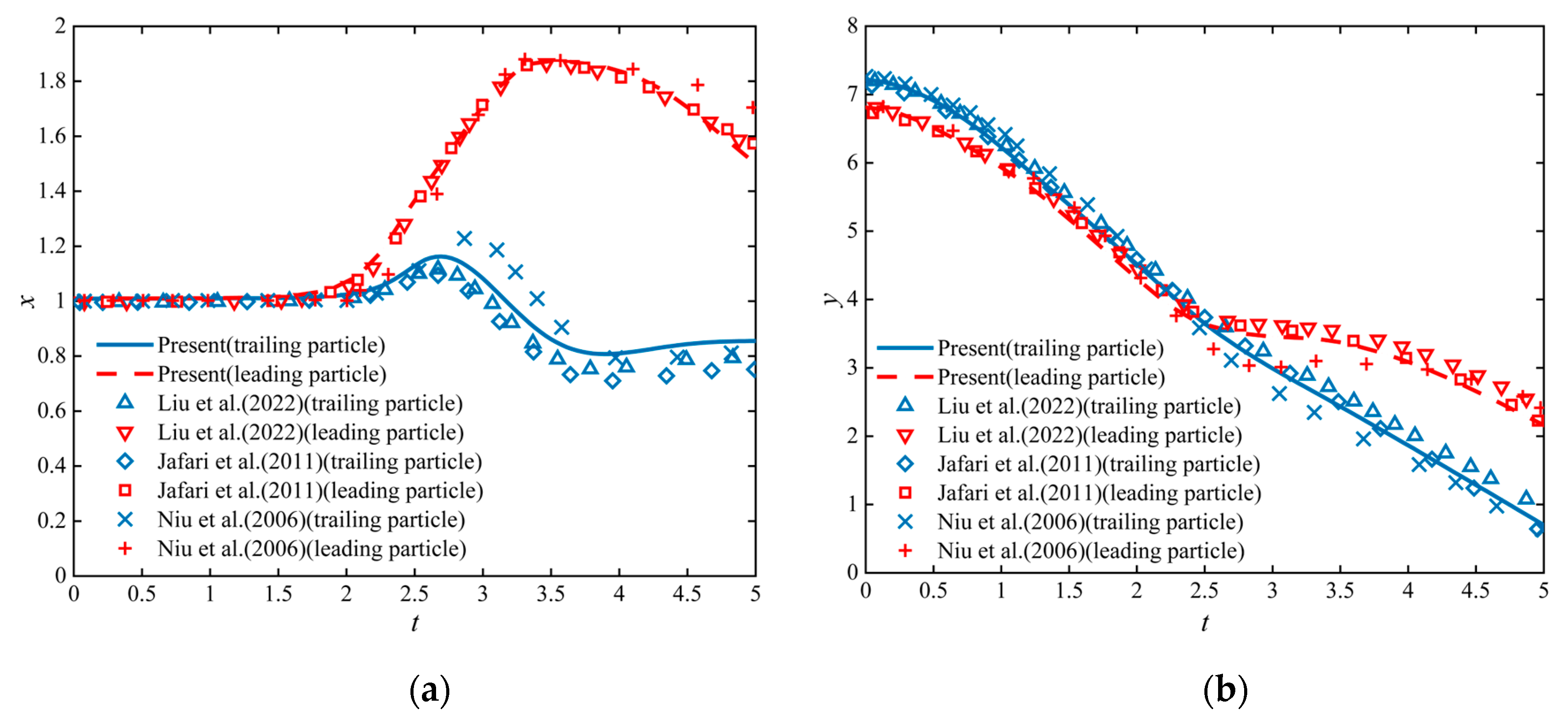
2.5. Model Validation

The DKT problem of two circular particles under gravity is used to verify the effectiveness of the method adopted in this paper. In a computational domain of 200 × 800 filled with stationary fluid, a circular particle with zero initial velocity is released at positions (100.9, 721) and (101, 681). Non-slip boundary conditions are applied to all walls in the computational domain. The important dimensionless number in particle sedimentation problems is the Archimedes number $\mathrm{Ar}=\sqrt{g{D_p}^3\left({\rho }_p-{\rho }_f\right)/\left({{\nu }_f}^2{\rho }_f\right)}$ [35]. In the calculation, the fluid density and viscosity are set to ${\rho }_f=1.0$ and ${\nu }_f=0.05$, respectively. The particle density and diameter are set to ${\rho }_p=1.01$ and $D_p=20$, respectively. In this simulation, Ar = 28, and the gravitational acceleration is calculated to be g = 0.0245. It should be noted that, unless otherwise specified, the physical quantities in this paper are all taken in lattice units.

The instantaneous positions of the two particles during drafting, kissing, and tumbling are shown in Figure 2a. It can be seen that as the two particles settle, the trailing particle first approaches the leading particle due to the low-pressure wake generated by the leading particle. Then, the trailing particle with higher velocity makes contact with the leading particle, and finally, the two particles tumble and separate from each other. These three processes are known as drafting, kissing, and tumbling. Figure 2b shows the contour of fluid velocity in the y-direction. It can be seen that as the particles settle, the region with the highest downward velocity of the fluid in the cavity is located behind the particle movement, while the region with the highest upward velocity of the fluid is on the sides behind the particle movement. The streamlines corresponding to these three processes are shown in Figure 2c. The fluid is dragged by the sedimentation of the two particles and forms vortices on the left and right sides. When the two particles kiss, the vortices on both sides further approach the particle contact area. Then, as the particles tumble and separate, vortices are generated around each particle, and the blocking effect of the right wall causes the fluid to form vortices only on the left side of the leading particle. Figure 3 shows the instantaneous curves of the horizontal and vertical positions of the centers of the two particles calculated in this paper, as well as the results calculated by others. It can be seen from the figure that the results of this paper are in good agreement with the results of others, which verifies that the method used in this paper can effectively handle the particle sedimentation problem.

3. Results and Discussion

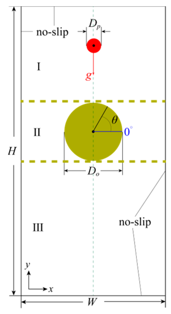
3.1. The Sedimentation of a Single Circular Particle in a Cavity Containing an Obstacle

The sedimentation of a single circular particle in a cavity containing a circular obstacle was simulated. The overall computational domain is W × H = 400 × 800, and non-slip solid wall boundary conditions are applied to the four walls of the cavity. The particle is released in a stationary fluid. As shown in Figure 4, the diameters of the obstacle and the particle are set to D_o = 80 and D_p = 20, respectively. The densities of the particle and fluid are set to ${\rho }_p=1.01$ and ${\rho }_f=1$, respectively. The initial horizontal position and the vertical height of the particle’s center of mass are set to x_p = 200 and y_p = 721, respectively. The horizontal position and the vertical height of the obstacle’s center are set to x_o = 200 and y_o = 460, respectively. It is defined that the center angle θ of the obstacle surface increases in the counterclockwise direction, and the center angle θ = 0° of the obstacle center is horizontal to the right. The particle–obstacle eccentricity $\epsilon =\left|x_p-x_o\right|/D_o$ is defined. The fluid viscosity in the cavity is set to ${\nu }_f=0.05$, and the Archimedes number is set to Ar = 28. The values of parameters are listed in

Table 1. Values of parameters used in case3.1.

xp	yp	xo	yo	Do	Dp	${\mathsf{\rho }}_{\mathit{p}}$	${\mathsf{\rho }}_{\mathit{f}}$	ε	${\mathsf{\nu }}_{\mathit{f}}$
200	721	200	460	80	20	1.01	1	0	0.05

. Additionally, as shown in Figure 4, the cavity is divided into three regions in the vertical direction. Region II is the range covered by the obstacle in the vertical direction, with Region I above it and Region III below it.

The instantaneous position of a single circular particle’s sedimentation in a cavity containing a single obstacle is shown in Figure 5a, where the entire sedimentation process of the particle is divided into three stages: Stage 1 is the free-fall motion of the particle in Region I under the action of gravity; Stage 2 starts from the time the particle enters Region II and starts to make contact with the obstacle until it completely leaves, during which the particle’s sedimentation trend is slowed down due to the obstruction of the obstacle, and the particle will tumble around the obstacle, resulting in translational motion; and Stage 3 is the free-fall motion of the particle until it sinks to the bottom after entering Region III, and the particle comes to rest. From the local enlargement in Figure 5b, it can be seen that after entering Region II, the particle rotates clockwise around the obstacle, then changes from clockwise to counterclockwise rotation, and after a period of free-fall, its rotation disappears, and it sinks until it reaches the bottom. The velocity in y-direction contour at different times during the particle sedimentation process is shown in Figure 5c, from which it can be seen that the region with the highest downward velocity of the fluid in the cavity is always behind the particle movement. When the particle enters Region II, the downward velocity of the fluid decreases due to the obstruction of the obstacle, and when the particle enters Region III, this velocity gradually increases. Figure 5d shows the streamline distribution near the particle, from which it can be seen that the sedimentation of the particle drives the surrounding fluid to form vortices. When sedimentation occurs in Region I, the vortices are symmetrically distributed on the left and right sides of the particle. As the particle gradually approaches the obstacle, the vortices are squeezed by the obstacle and gradually converge above the particle. After entering Region II, due to the obstruction of the obstacle, the left vortex stays above the obstacle, and the right vortex moves downward with the particle. After the particle enters Region III, a new vortex is generated on its left side, and its size gradually increases as the particle moves away from the obstacle.

An instantaneous velocity curve in the y-direction of a single particle during sedimentation in a cavity containing an obstacle is shown in Figure 6a. In Stage 1, due to free-fall, the velocity in the y-direction of the particle increases rapidly. In Stage 2, when the particle reaches the obstacle, the velocity in the y-direction decreases rapidly and even shows a rebound trend. Then, due to the obstacle occupying the particle’s sedimentation path, the particle tumbles along the surface of the obstacle until it leaves, during which the velocity in the y-direction of the particle increases slowly from zero. In Stage 3, after the particle bypasses the obstacle and begins to free-fall again until it sinks to the bottom, the velocity in the y-direction of the particle increases to the maximum value and then maintains a period of uniform motion until the velocity is zero. An instantaneous velocity curve in the x-direction of a single particle during sedimentation in a cavity containing an obstacle is shown in Figure 6b. In Stage 1, the particle falls freely without any translational trend, and the velocity in the x-direction is zero. In Stage 2, when the particle reaches the obstacle and moves around it, the velocity in the x-direction of the particle increases to the maximum value and then decreases, followed by a small increase. In Stage 3, due to inertia, the particle continues to translate to the right for a certain distance, during which the velocity in the x-direction decreases until the particle sinks to the bottom, and the velocity in the x-direction tends to zero.

An instantaneous curve of the angular velocity during the sedimentation process of the particle is shown in Figure 7. In Stage 1, the angular velocity remains zero throughout, indicating that the particle undergoes a purely vertical free-fall under gravity without rotational tendency before coming into contact with the obstacle. This aligns with the theoretical expectations of flow field symmetry and the absence of external torque. In Stage 2, when the particle comes into contact with the obstacle, the obstacle disrupts the flow field symmetry, creating a velocity gradient disparity between the two sides of the particle. This velocity difference generates left-to-right shear stress on the particle surface, forming a net torque that drives clockwise tumbling around the obstacle. During this process, the tangential friction at the contact point opposes the particle’s motion, further amplifying the clockwise torque and causing the clockwise rotation speed to reach its peak value. Simultaneously, the particle’s center-of-mass offset induces a counterclockwise torque component from the normal contact force, and the competition between these two torques results in the angular velocity gradually recovering from negative (clockwise) to positive (counterclockwise) values. After the particle detaches from the obstacle surface, the accumulated counterclockwise torque drives continued counterclockwise rotation. At this stage, the vortex lines in the flow field on the particle’s right side also exhibit counterclockwise orientation. According to the Magnus effect, the particle’s rotation entrains surrounding fluid via viscous interaction, creating a high-velocity flow zone on its right side, which reduces pressure on the right side (Bernoulli principle), amplifies the counterclockwise torque, and accelerates the counterclockwise rotation to its peak value. Finally, in Stage 3, the torque from fluid viscous resistance gradually counteracts the counterclockwise torque, causing the rotation speed to peak and subsequently decay. As the particle resumes free settling, its angular velocity progressively approaches zero.

Next, the force experienced by the obstacle is discussed when the particle moves around its surface, in order to better understand the interaction between the particle and the obstacle. Figure 8 shows the force in y-direction and x-direction distributions on the obstacle surface at three different times due to the particle’s action, from which it can be seen that the particle exerts force on a certain area of the obstacle surface. In addition, as shown in Figure 8a, when the particle begins to come into contact with the obstacle, the contact surface is subjected to a downward force from the particle; that is, at this time, the obstacle exerts an upward supporting force on the particle, which lasts until the particle leaves the obstacle surface. As shown in Figure 8b, when the particle comes into contact with the obstacle, the direction of the force on the contact area is horizontally to the left, so the obstacle exerts a force horizontally to the right on the particle, pushing the particle to move to the right and lasting until the particle leaves the obstacle surface. Since the particle is settling under the action of gravity, the y-direction is the main force-bearing direction. According to the scale given in Figure 8, the force in the y-direction experienced by the contact area of the obstacle is roughly one order of magnitude larger than the force in the x-direction.

The instantaneous curves of the maximum and minimum central angles corresponding to the region acted upon by the particle and the forces in two directions are shown in Figure 9. It can be seen from the figure that with the increase in time, both the maximum and minimum central angles show a downward trend, and the difference between the two becomes smaller and smaller, indicating that during the process of the particle contacting and gradually leaving the obstacle, the region on the obstacle surface acted upon by the particle also gradually becomes smaller. In addition, throughout the entire process of contact with the particle, the force in the y-direction experienced by the obstacle is always acting downward, with its peak occurring at the initial moment of contact between the obstacle and the particle and then gradually decreasing with time. The force experienced in the x-direction is always to the left, with its value showing a process of first decreasing, then increasing to a peak, and then decreasing again.

After the translation, the rotation of the particle during sedimentation and the force exerted on the obstacle are discussed. The movement of the particle and the change in the force exerted on the obstacle during sedimentation are observed by changing three factors: particle–obstacle eccentricity, the particle–obstacle diameter ratio, and the particle diameter to obstacle spacing ratio.

3.2. Influence of Particle–Obstacle Eccentricity on Particle Sedimentation

In this section, the initial vertical height of the particle’s center of mass is kept constant at y_p = 721, and the particle–obstacle eccentricity $\epsilon$ is varied by changing the horizontal position of the particle’s center of mass. $\epsilon$ = 0, 0.125, 0.25, and 0.375 are selected, with all other parameters remaining the same as those in Section 3.1. The values of parameters are listed in

Table 2. Values of parameters used in case3.2.

	ε	xp	xo	yo	Do	Dp	${\mathsf{\rho }}_{\mathit{p}}$	${\mathsf{\rho }}_{\mathit{f}}$	${\mathsf{\nu }}_{\mathit{f}}$
Case3.2.a	0	200	200	460	80	20	1.01	1	0.05
Case3.2.b	0.125	210	200	460	80	20	1.01	1	0.05
Case3.2.c	0.25	220	200	460	80	20	1.01	1	0.05
Case3.2.d	0.375	230	200	460	80	20	1.01	1	0.05

. Changing $\epsilon$ has little effect on the sedimentation process of the particle in Stage 1 and Stage 3. Therefore, only the sedimentation process in Stage 2 is focused on.

Streamlines around the particle at different times in Stage 2 under different conditions of $\epsilon$ are shown in Figure 10. It can be seen from the figure that the overall trend in the streamline distribution around the particle is consistent. The difference is that as the $\epsilon$ value increases, when the particle enters Region II, the asymmetry in the distribution of vortices on both sides of the particle gradually increases. When the particle moves around the obstacle, the distance between the vortex centers on both sides decreases, and the vortex centers move closer to the particle, indicating that the obstruction effect of the obstacle on the particle is weakening. When the particle is about to leave Region II, the vortex on the left side of the particle becomes larger, indicating that the fluid disturbance effect is enhanced.

The instantaneous velocity curves in the y-direction and x-direction of the particle during sedimentation under different conditions of $\epsilon$ are shown in Figure 11. It can be seen that the overall trend in the instantaneous velocity curves is consistent. The difference is that as the $\epsilon$ value increases, the obstruction effect of the obstacle on the particle weakens. The extreme value of the velocity in the y-direction when the particle hits the obstacle increases, allowing the particle to enter Stage 3 for free-fall earlier until it sinks to the bottom. On the other hand, as the $\epsilon$ value increases, the extreme value of the horizontal velocity to the right of the particle in Stage 2 increases, and the time to reach the extreme value is advanced. In addition, the fluctuation in the velocity in the x-direction when the particle continues to move horizontally to the right after leaving the obstacle weakens. This increase in the extreme value of y-direction velocity and the weakening of x-direction velocity fluctuations under high-ε conditions aligns with the shortened particle–obstacle interaction duration observed by Shi et al. [39] in their study of particle sedimentation through straight-arranged porous media. Linearly arranged obstacles (analogous to the high-ε condition in this study) similarly reduce lateral velocity oscillations and improve vertical settling efficiency by reducing structural tortuosity.

The process of rotational direction changing and the corresponding time during particle sedimentation under different conditions of $\epsilon$ are shown in Figure 12. It can be seen from the figure that as the $\epsilon$ value increases, the time when the particle comes into contact with the obstacle is delayed, and the time for the particle to move around the obstacle is shortened, which results in the delay of the time when the particle starts to rotate clockwise and the shortening of the time when it maintains clockwise rotation. According to this law, with increasing $\epsilon$ values, particles initiate counterclockwise rotation earlier after leaving the obstacle, while the duration of this rotational maintenance shows a proportional decrease.

The instantaneous curves of the angular velocity of the particle during sedimentation under different conditions of ε are shown in Figure 13. It can be seen from the figure that the overall trend in the angular velocity change is consistent. The difference is that as ε increases, the time during which the particle rotates as a whole is shortened, the peak value of the clockwise angular velocity gradually decreases, and the time of appearance of the peak value is delayed. This is because the larger the eccentric distance, the more the particle deviates from the center of the obstacle, and circumnavigation assistance is reduced. After the particle leaves the surface of the obstacle, the direction of rotation changes from clockwise to counterclockwise, and the angular velocity changes from negative to positive. With the increase in ε, the peak value of the counterclockwise rotation angular velocity decreases, and the time of direction change is advanced, indicating that the larger the ε value, the weaker the obstruction effect of the obstacle on the particle, and the particle’s angular velocity can decay to zero earlier.

The instantaneous curves of the maximum and minimum central angles corresponding to the region of the obstacle acted upon by the particle under different conditions of $\epsilon$ are shown in Figure 14. It can be seen from the figure that with the increase in time, the maximum and minimum central angles corresponding to the region of the obstacle acted upon by the particle, as well as the difference between the two, all show a trend of decreasing from large to small under different conditions of $\epsilon$. The difference is that as the $\epsilon$ value increases, the maximum and minimum central angles when the particle begins to come into contact with the obstacle decrease, while the central angles when the particle leaves the obstacle increase. In addition, as the $\epsilon$ value increases, the time during which the obstacle is acted upon by the particle shortens.

The instantaneous curves of the force exerted on the obstacle by the particle under different conditions of $\epsilon$ are shown in Figure 15. It can be seen that the force in the y-direction is always downward, and the trend in change is consistent. The difference is that as the $\epsilon$ value increases, the peak force in the y-direction exhibits an initial increase followed by a subsequent decrease. The force in the x-direction is always to the left. When $\epsilon$ = 0, the force in the x-direction changes relatively gently over time. However, when the $\epsilon$ value is not zero, the peak force in the x-direction manifests at the initial contact moment between the particle and obstacle, demonstrating a non-monotonic trend characterized by an initial increase followed by a progressive decrease with the $\epsilon$ value increasing.

3.3. The Influence of the Particle–Obstacle Diameter Ratio on Particle Sedimentation

To investigate the effects of the particle–obstacle diameter ratio on particle sedimentation, the particle–obstacle diameter ratio is defined as $D_r=D_o/D_p$, with the particle diameter fixed at D_p = 20 and the particle–obstacle eccentricity $\epsilon$ = 0. The variation in D_r is achieved by changing the obstacle diameter D_o, with D_r values selected as D_r = 2, 4, and 6, while the other parameters remain the same as those in Section 3.1. The values of parameters are listed in

Table 3. Values of parameters used in case3.3.

	Dr	Do	Dp	xo	yo	ε	${\mathsf{\rho }}_{\mathit{p}}$	${\mathsf{\rho }}_{\mathit{f}}$	${\mathsf{\nu }}_{\mathit{f}}$
Case3.3.a	2	40	20	200	460	0	1.01	1	0.05
Case3.3.b	4	80	20	200	460	0	1.01	1	0.05
Case3.3.c	6	120	20	200	460	0	1.01	1	0.05

. As in Section 3.2, the focus here is solely on the particle motion process in Stage 2.

The streamline diagrams of a particle at different moments in Stage 2 under different conditions of D_r are shown in Figure 16. It can be seen that the overall trend in the streamline distribution near the particle is consistent. The difference lies in that as D_r increases, the time at which vortices regenerate on the left side of the particle is delayed, and the size of the vortices on the right side of the particle increases.

The instantaneous velocity curves in the y-direction and x-direction during the sedimentation process of a particle under different conditions of D_r are shown in Figure 17. It can be observed that the overall trend in the velocity curves is consistent. The difference lies in that as D_r increases, the extremum velocity in the y-direction when the particle encounters obstacles decreases, the moment when the particle enters Stage 3 is delayed, and the time at which the particle reaches the maximum rightward horizontal velocity in Stage 2 is also delayed. The observed reduction in the y-direction velocity extremum and prolonged Stage 2 transitions under high-D_r conditions align with the dynamics reported by Shi et al. [39] for particles settling in porous media with varying obstacle diameters. Specifically, when particles settle through porous media containing larger obstacles (analogous to higher D_r in this study), the average sedimentation velocity extremum of multiple particles decreases, accompanied by delayed velocity recovery similar to that observed here. The enlarged obstacles intensify local velocity gradients, thereby extending the timescales for particle reorientation and energy redistribution.

The instantaneous curves of the rotational angular velocity of particles during the sedimentation process under different conditions of D_r are shown in Figure 18. It can be observed from the figure that the overall trend in the particle’s rotational angular velocity is consistent. The difference lies in that as D_r increases, the extremum of the particle’s angular velocity during clockwise rotation around the obstacle in Stage 2 decreases. After the particle leaves the surface of the obstacle, the rotation direction changes from clockwise to counterclockwise, and the extremum of the angular velocity during counterclockwise rotation increases.

The instantaneous curves of the maximum and minimum central angles corresponding to the area of the obstacle subjected to particle action under different conditions of D_r are shown in Figure 19. It can be observed from the figure that with the increase in time, both the maximum and minimum central angles, as well as the difference between them, show a trend of decreasing. The difference lies in that as D_r increases, the maximum central angle when the particle begins to come into contact with the obstacle decreases, while the minimum central angle increases. Moreover, the central angle increases when the particle leaves the obstacle. Additionally, as the diameter ratio increases, the starting time of the particle’s action on the obstacle advances, the ending time is delayed, and the total action time is extended.

The instantaneous curves of the force applied by the particles on the obstacle under different conditions of D_r are shown in Figure 20. It can be observed that the force in the y-direction is consistently downward, while the force in the x-direction is consistently to the left. The instantaneous curves exhibit a consistent trend. The difference lies in that, with the increase in D_r, the peak force in the y-direction first increases and then decreases. Meanwhile, the peak force in the x-direction remains roughly the same, but the timing of when the peak is reached is progressively delayed.

3.4. Influence of the Particle Diameter to Obstacle Spacing Ratio on Particle Sedimentation

Subsequently, an obstacle of the same size is placed horizontally to the right of the existing obstacle, with a horizontal gap of d_c between them. The particle will continue to settle through this gap after leaving the left-side obstacle. The effects of the presence of this gap on particle sedimentation are analyzed in this section. The particle diameter–obstacle spacing ratio is defined as $R=d_c/D_p$, with $\epsilon$ = 0 and D_r = 4 fixed. The variation in R is achieved by adjusting d_c. The values selected for R are 1.095, 1.115, 1.135, and 1.155, while the other parameters remain the same as those in Section 3.1. The values of parameters are listed in

Table 4. Values of parameters used in case3.4.

	R	dc	Dp	xo	yo	ε	${\mathsf{\rho }}_{\mathit{p}}$	${\mathsf{\rho }}_{\mathit{f}}$	${\mathsf{\nu }}_{\mathit{f}}$
Case3.4.a	1.095	21.9	20	200	460	0	1.01	1	0.05
Case3.4.b	1.115	22.3	20	200	460	0	1.01	1	0.05
Case3.4.c	1.135	22.7	20	200	460	0	1.01	1	0.05
Case3.4.d	1.155	23.1	20	200	460	0	1.01	1	0.05

. Similarly, the focus here is solely on the sedimentation process of the particle in Stage 2.

The streamline diagrams of particle sedimentation at different times in Stage 2 under different conditions of R are shown in Figure 21. From the diagram, it can be observed that the overall trend in the streamline distribution near the particle is consistent. After the particle passes through the gap between the two obstacles, new vortices are generated on both sides. Since the particle is closer to the left-side obstacle, the size of the new vortex generated on the left side will be smaller.

The instantaneous velocity curves in the y-direction and x-direction during the particle sedimentation process under different conditions of R are shown in Figure 22. From the figure, it can be observed that the instantaneous velocity curve in the y-direction exhibits a downward trend, first decelerating and then accelerating in Stage 2. In the corresponding period, the instantaneous velocity curve in the x-direction shows a negative change. This indicates that when particle pass through the gap between obstacles, it is influenced by the right-side obstacle, which delays its sedimentation process and disrupts the trend of accelerated falling. The particle’s settling velocity decreases first and then increases while also moving to the left. Furthermore, upon further observation, it can be seen that as R increases, the degree of delay in the sedimentation process of the particle weakens, indicating that the influence of the right-side obstacle decreases.

The instantaneous rotational angular velocity curves during the sedimentation of particles under different conditions of R are shown in Figure 23. It can be observed that the overall trend in the instantaneous angular velocity curve during the sedimentation process in Stage 2 is consistent. The particle exhibits a clockwise rolling motion, with the angular velocity first showing a slow process of increasing and then decreasing, followed by a rapid process of increasing and then decreasing. Afterward, the particle transitions from clockwise to counterclockwise rotation. As R increases, the second peak of the particle’s clockwise rotational angular velocity gradually decreases, indicating that the influence of the right-side obstacle on the particle weakens.

Next, an analysis of the particle interaction with the left-side obstacle is conducted. The instantaneous curves of the maximum and minimum central angles corresponding to the region of particle interaction with the left-side obstacle under different conditions of R are shown in Figure 24a. From the figure, it can be observed that the instantaneous curve is interrupted, indicating that the left-side obstacle is affected by settling particles during two distinct time periods. The occurrence of the second period is due to the particles being influenced by the lateral force from the right-side obstacle after leaving the left-side obstacle, leading to a second interaction with the left-side obstacle. Upon comparison, it is found that the instantaneous curve of the first period in Figure 24a is identical to that in Figure 9a, indicating that the change in R has no effect on the particles during the first period.

Afterwards, an analysis of the variation process of the maximum and minimum central angles corresponding to the region of particle interaction with the left-side obstacle during the second period is conducted, with the corresponding instantaneous curves shown in Figure 24b, which shows a local enlargement of the instantaneous curve in the boxed area of Figure 24a. From the figure, it can be observed that as time progresses, the central angles under different conditions of R all show a trend of decreasing from large to small. The difference lies in that, with the increase in R, the start time of particle interaction with the left-side obstacle is delayed, while the end time is advanced. Additionally, a plateau phase appears in each instantaneous curve, indicating that during this period, the particle position remains mostly unchanged. Furthermore, as R increases, the duration of the plateau phase shortens.

As mentioned earlier, the presence of the right-side obstacle only affects the interaction between the particles and the left-side obstacle during the second period. Therefore, only the instantaneous force curves on the left-side obstacle during the second period under different conditions of R are shown below. As shown in Figure 25, it can be seen that the trend in force variation in the y-direction is consistent, with a downward force that gradually increases and then decreases, followed by an upward force that gradually increases and then decreases. Similarly, the force variation trend in the x-direction is also consistent, with a leftward force that gradually increases and then decreases. Moreover, as R increases, both the force and its peak values decrease, indicating that as R increases, the lateral force exerted on the particles by the right-side obstacle gradually weakens. When the gap between the two obstacles exceeds a certain threshold (R ≥ 1.195), the presence of the right-side obstacle no longer exerts any effect on the particles. This result shows a significant correlation with the threshold effect of dual-obstacle spacing on topological structure stability studied by Santos et al. [40]. When the dual-obstacle spacing exceeds the critical threshold (h > 6.25 μm), the flow channel constraint on torons passing through the dual obstacles becomes ineffective. The observed attenuation of lateral force on particle with increasing R in this study is consistent with the phenomenon of reduced elastic stress on torons as spacing increases.

4. Conclusions

The immersed boundary–lattice Boltzmann method is used in this paper to simulate the sedimentation of a single particle in a cavity with an obstacle under the condition of Archimedes number Ar = 28. The following conclusions are reached:

(1)

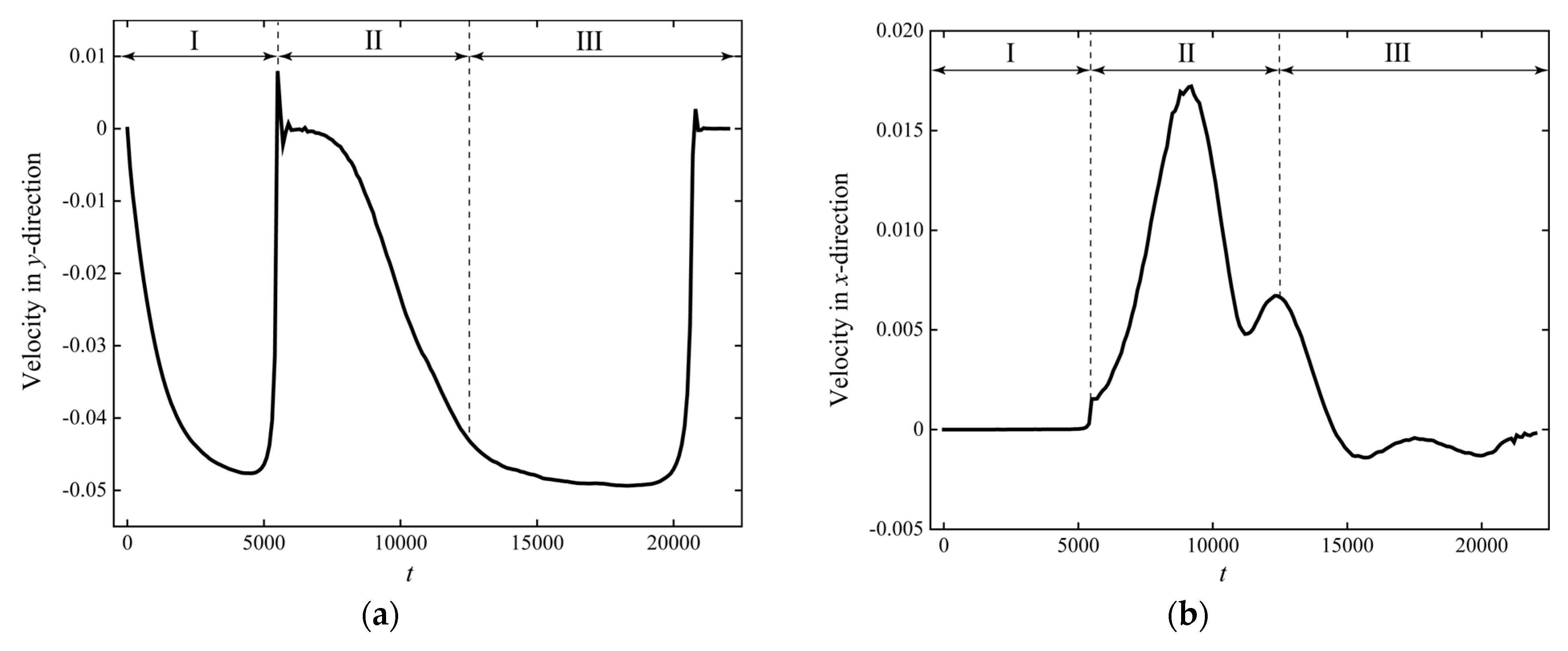
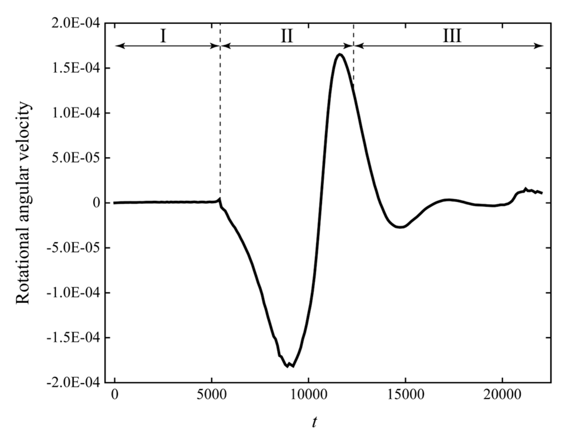
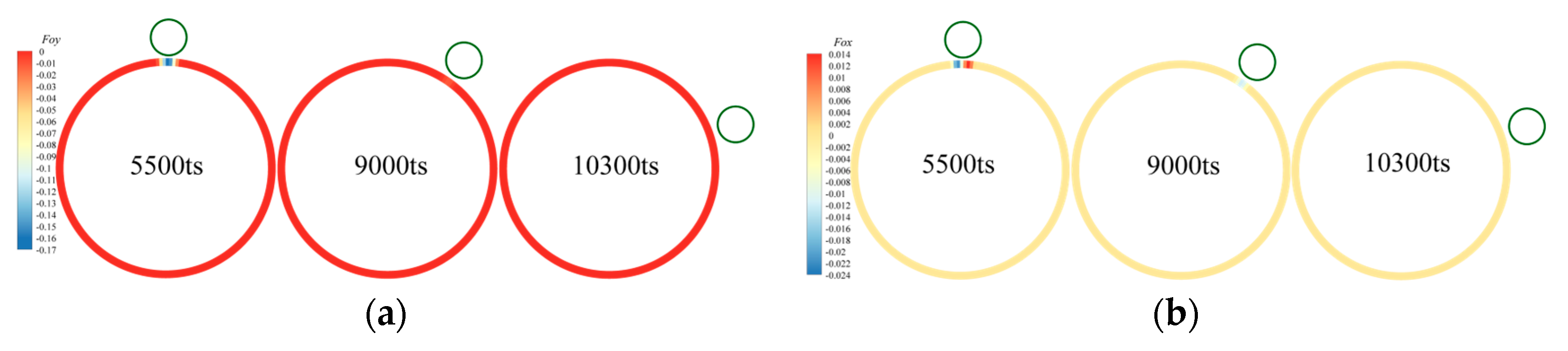
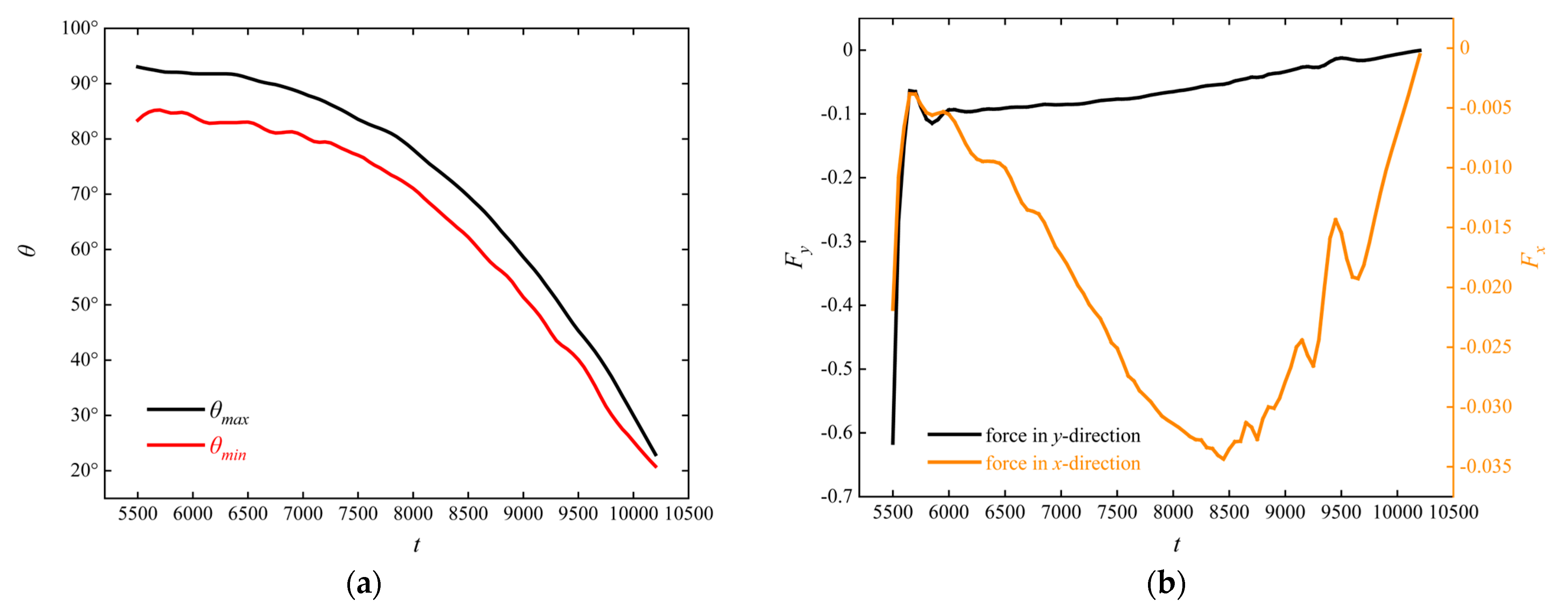
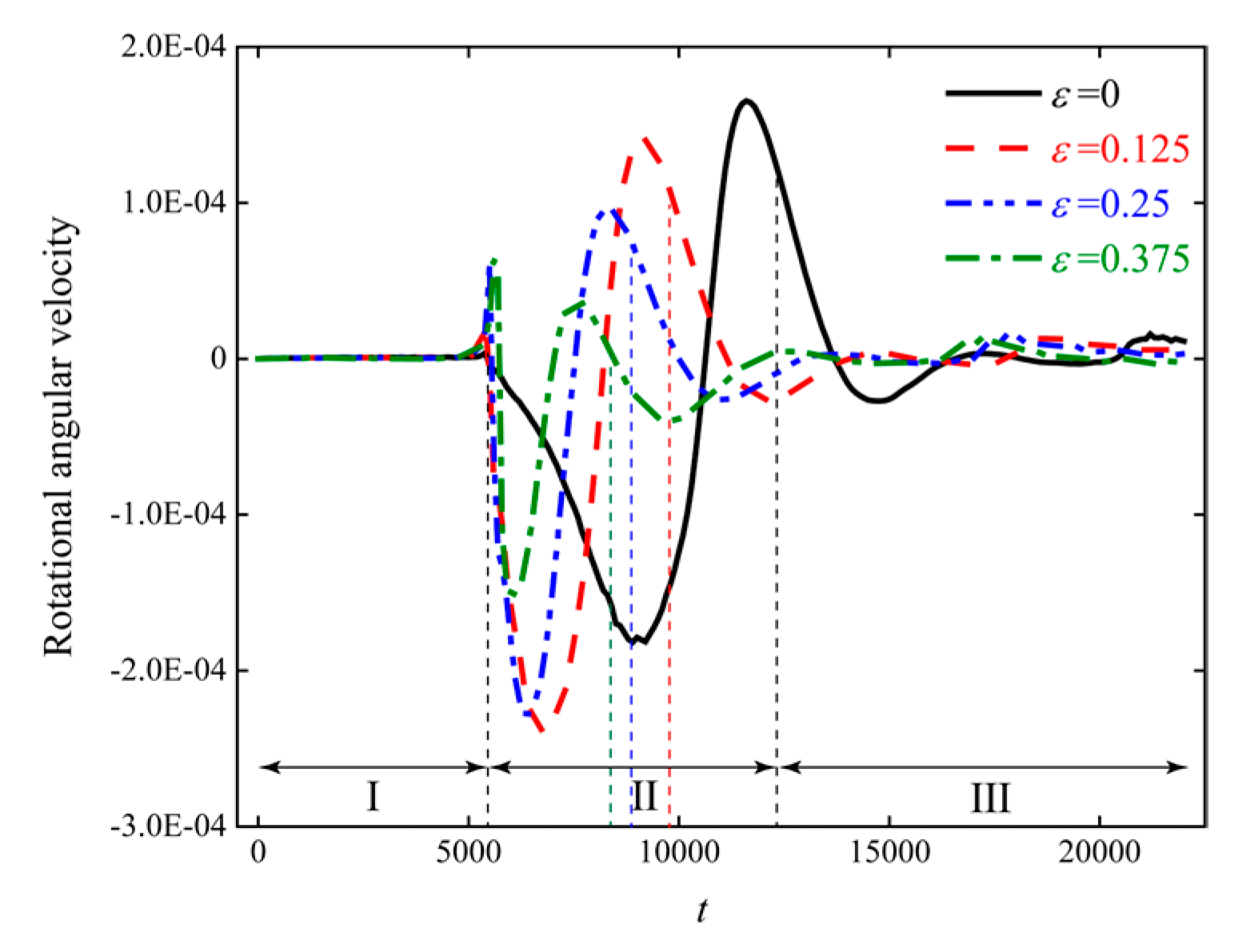
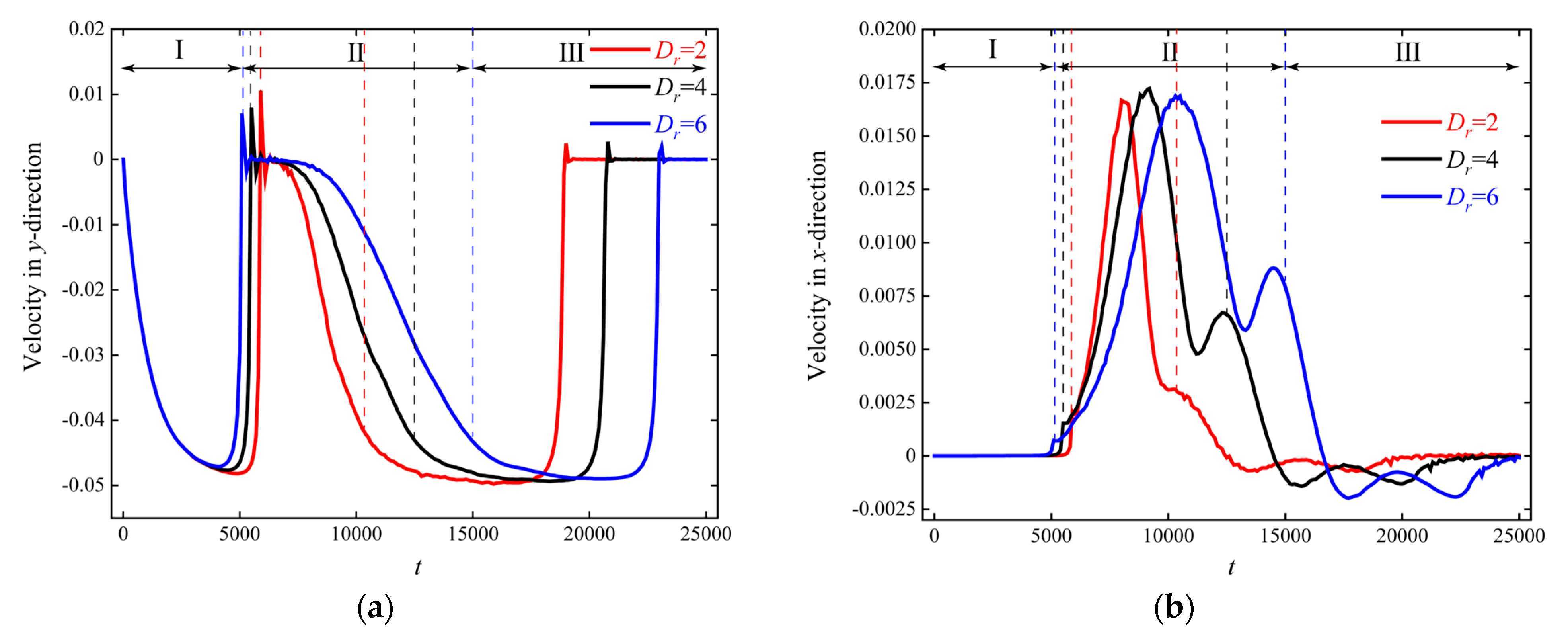
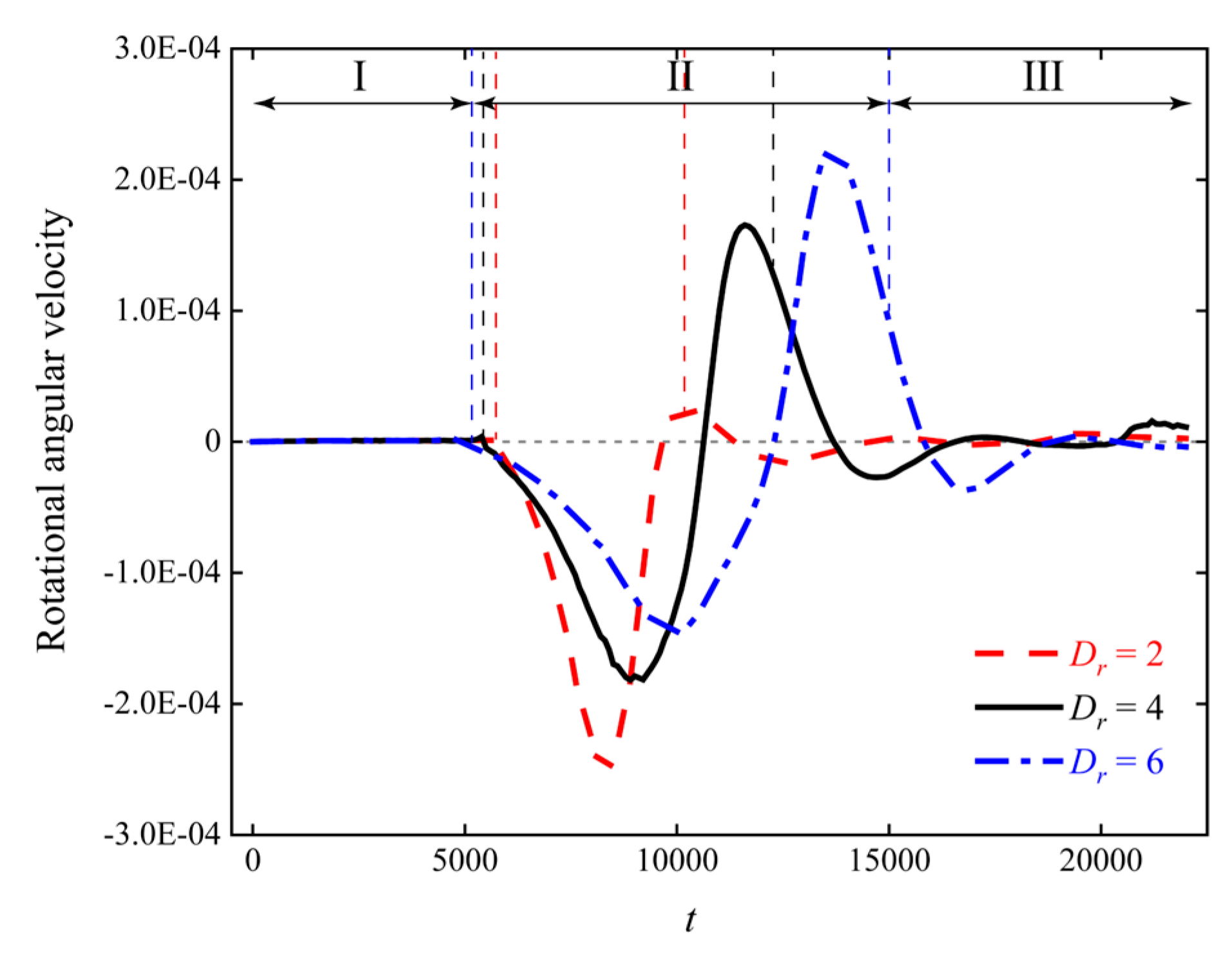
The sedimentation process of the particle in a cavity with an obstacle can be divided into three stages. During the entire sedimentation period, the particle’s velocity in the y-direction first increases, then decreases, and finally increases again until the particle settles at a constant speed. The velocity in the x-direction shows an initial increase followed by a decrease. In Stage 2, the particle first rotates clockwise around the obstacle and then changes its rotational direction. During this period, the obstacle provides both support and propulsion to the particle, with the support force being roughly an order of magnitude greater than the propulsion force.

(2)

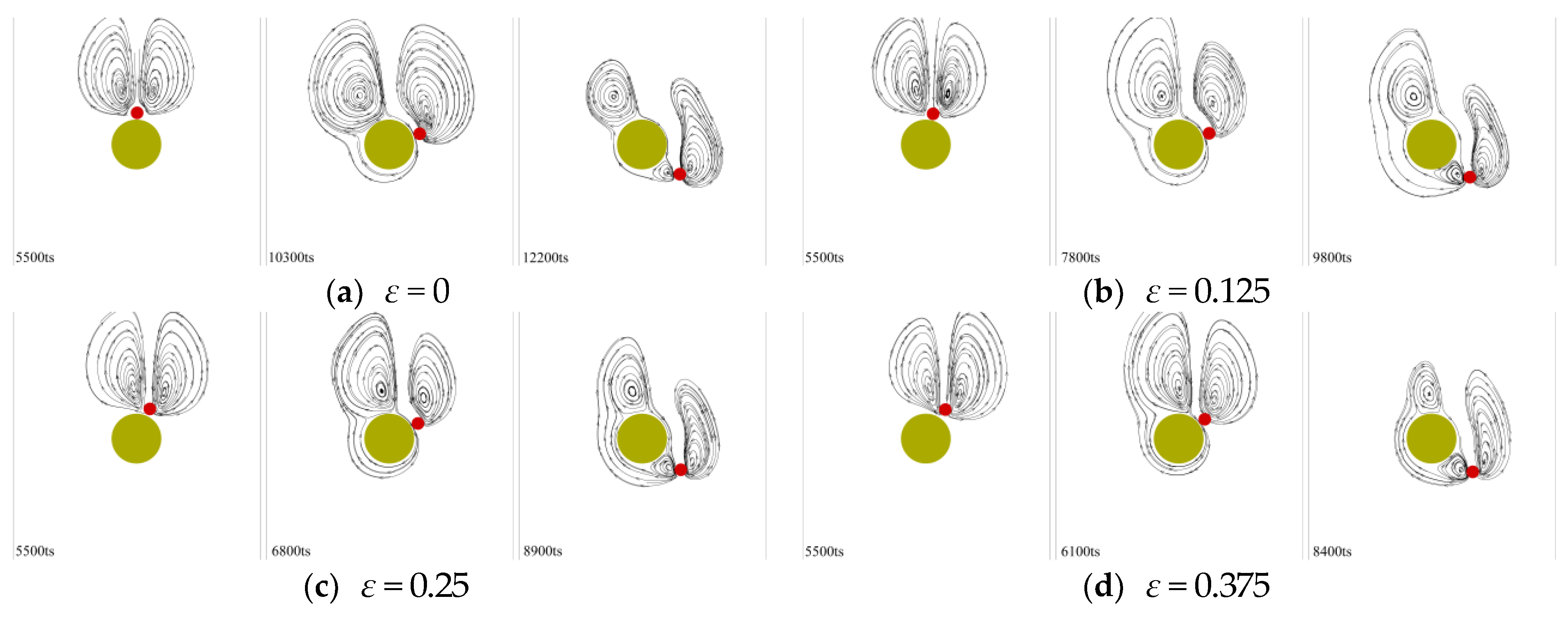
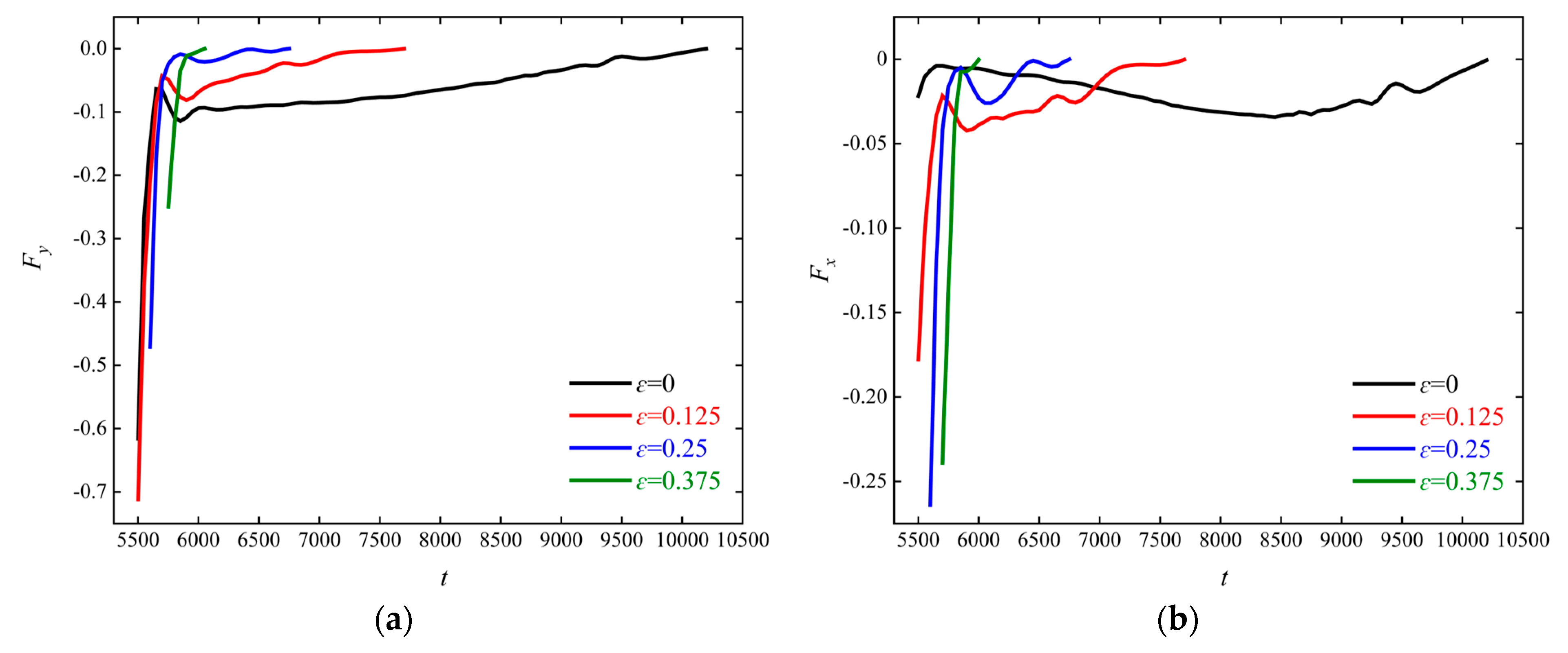
As the particle–obstacle eccentricity $\epsilon$ increases, the extreme values of the particle’s velocity in the y-direction and x-direction in Stage 2 both increase, while the area affected by the particle on the obstacle decreases, and the duration of the interaction shortens.

(3)

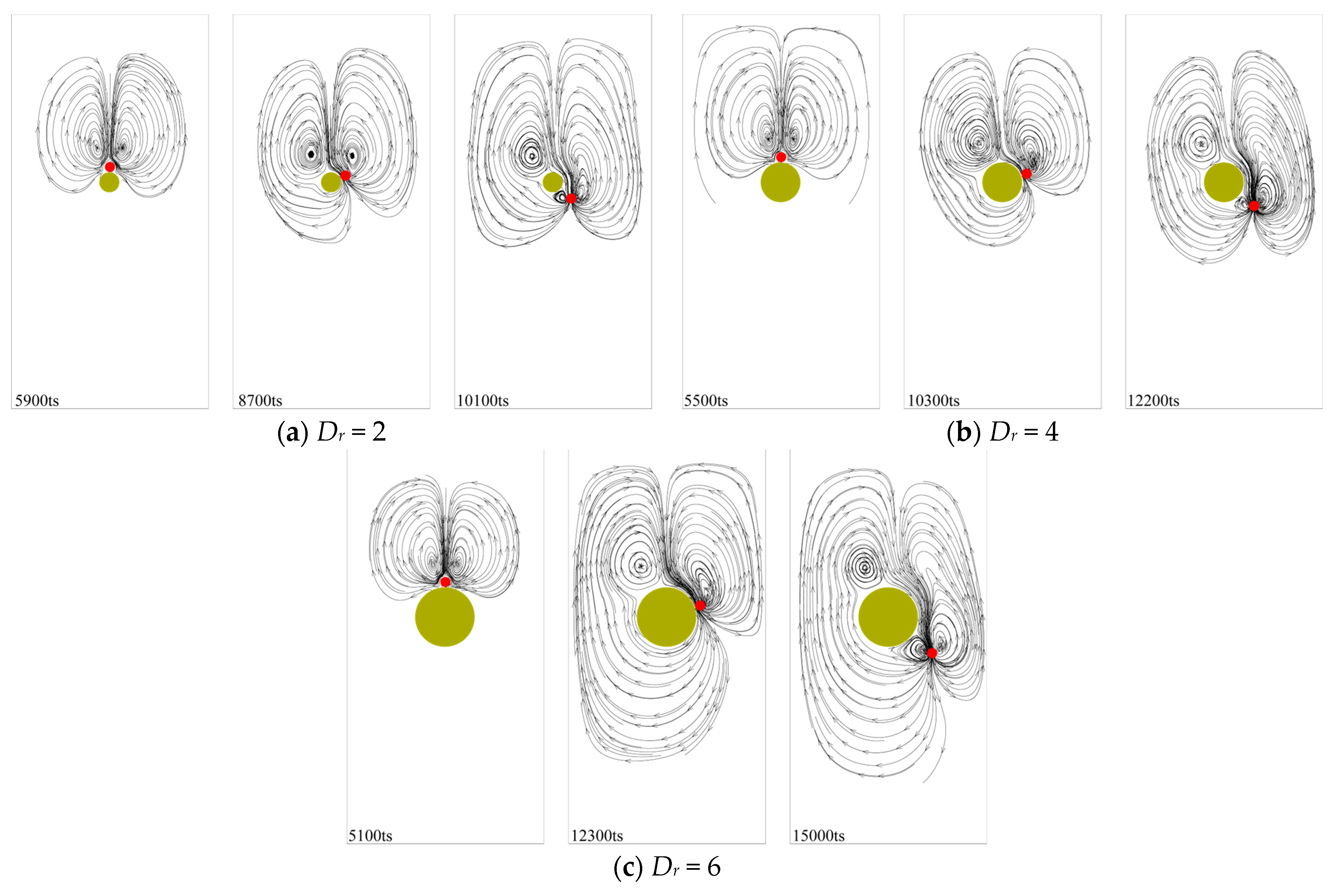
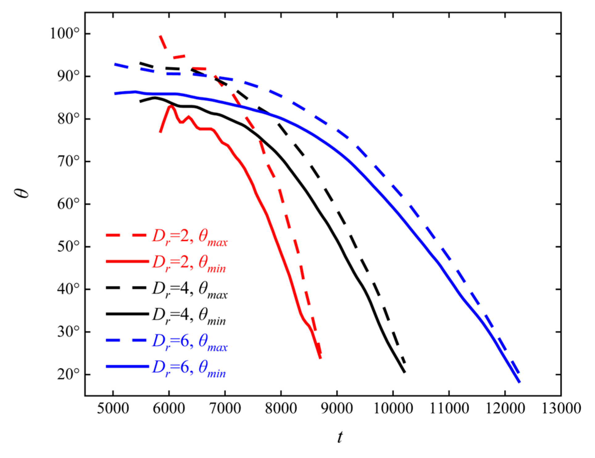
As the particle–obstacle diameter ratio D_r increases, the extreme value of the particle’s velocity in the y-direction in Stage 2 decreases, the moment when the velocity in the x-direction reaches its extreme value is delayed, the area affected by the particle on the obstacle increases, and the duration of the interaction is prolonged.

(4)

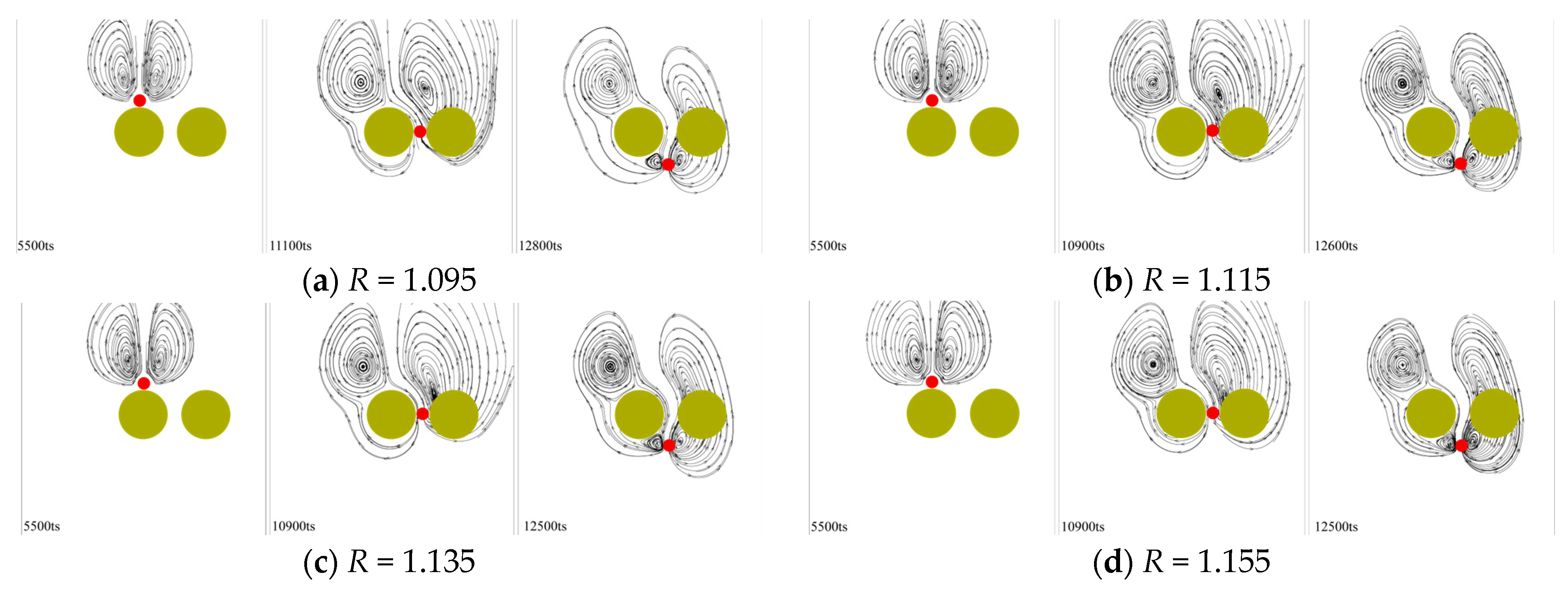
When a particle settles through the gap between two obstacles, if the particle diameter to obstacle spacing ratio R is small, the influence of the far-side obstacle causes the particle to exhibit a phenomenon where its motion trend is disrupted and then restored in a shorter period during in Stage 2, accompanied by a secondary interaction with the near-side obstacle. As R increases, the influence of the far-side obstacle gradually decreases, and after surpassing a certain threshold (R ≥ 1.195), the effect of the far-side obstacle on the settling particle disappears.

References

- Hamisi, R.; Renman, A.; Renman, G.; Wörman, A.; Thunvik, R. Treatment efficiency and recovery in sand filters for on-site wastewater treatment: Column studies and reactive modelling. J. Clean. Prod. 2024, 462, 142696. [Google Scholar] [CrossRef]
- Zhou, F.Q.; Guo, Y.N.; Qian, H.; Fu, S.C.; Yuan, H.X. Effect of wall roughness on particle deposition on the outer wall of the vortex finder in a cyclone separator. Adv. Powder Technol. 2024, 35, 104428. [Google Scholar] [CrossRef]
- Zhu, D.Y.; Liu, Q.Y.; Meng, Q.Q.; Jin, Z.J. Enhanced effects of large-scale CO2 transportation on oil accumulation in oil-gas-bearing basins—Implications from supercritical CO2 extraction of source rocks and a typical case study. Mar. Pet. Geol. 2018, 92, 493–504. [Google Scholar] [CrossRef]
- Francesco, G.; Peter, M.; Judith, M.C.; Maurice, W.; Andrew, W.; Eann, A.P. Settling dynamics of nanoparticles in simple and biological media. R. Soc. Open Sci. 2021, 8, 210068. [Google Scholar]
- Li, Y.N.; Xu, Z.H.; Zhan, X.Y.; Zhang, T.B. Summary of experiments and influencing factors of sediment settling velocity in still water. Water 2024, 16, 938. [Google Scholar] [CrossRef]
- Zeng, G.; Jin, Y.; Qu, H.; Lu, Y.H. Experimental investigation and correlations for proppant distribution in narrow fractures of deep shale gas reservoirs. Pet. Sci. 2022, 19, 619–628. [Google Scholar] [CrossRef]
- Wang, Y.; Ren, X.F.; Zhao, J.P.; Chu, Z.K.; Cao, Y.X.; Yang, Y.; Duan, M.J.; Fan, H.; Qu, X.R. Experimental study of flow regimes and dust emission in a free falling particle stream. Powder Technol. 2016, 292, 14–22. [Google Scholar] [CrossRef]
- Fortes, A.F.; Joseph, D.D.; Lundgren, T.S. Nonlinear mechanics of fluidization of beds of spherical particles. Fluid Mech. 1987, 177, 467–483. [Google Scholar] [CrossRef]
- Zhang, G.D.; Gutierrez, M.; Li, M.Z. A coupled CFD-DEM approach to model particle-fluid mixture transport between two parallel plates to improve understanding of proppant micromechanics in hydraulic fractures. Powder Technol. 2017, 308, 235–248. [Google Scholar] [CrossRef]
- Su, J.; Zhou, C.J.; Jiang, C.; Zheng, M. The movement law and orientation control of rectangular particles in the viscous fluid domain based on IS-FEM. Adv. Powder Technol. 2022, 33, 103634. [Google Scholar] [CrossRef]
- Fernandes, C.; Faroughi, S.A. Particle-level simulation of magnetorheological fluids: A fully-resolved solver. Int. J. Multiph. Flow 2023, 169, 104604. [Google Scholar]
- Zou, L.; Sun, J.Z.; Sun, Z.; Yu, Z.B.; Zhao, H.B. Study of two free-falling spheres interaction by coupled SPH–DEM method. Eur. J. Mech. B Fluids 2022, 92, 49–64. [Google Scholar]
- Suh, Y.K.; Kang, J.F.; Kang, S.M. Assessment of algorithms for the no-slip boundary condition in the lattice Boltzmann equation of BGK model. Int. J. Numer. Methods Fluids 2008, 58, 1353–1378. [Google Scholar]
- Lin, C.L.; Videla, A.R.; Miller, J.D. Advanced three-dimensional multiphase flow simulation in porous media reconstructed from X-ray microtomography using the He–Chen–Zhang lattice Boltzmann model. Flow Meas. Instrum. 2010, 21, 255–261. [Google Scholar]
- Yang, F.; Jin, H.; Dai, M.Y. On the spreading behavior of a droplet on a circular cylinder using the lattice Boltzmann method. Chin. Phys. B 2024, 33, 064702. [Google Scholar]
- Yang, F.; Dai, M.Y.; Jin, H. Lattice Boltzmann simulation of cavitating flow in a two-dimensional nozzle with moving needle valve. Processes 2024, 12, 813. [Google Scholar] [CrossRef]
- Chen, W.Y.; Yang, F.; Yan, Y.H.; Guo, X.Y.; Dai, R.; Cai, X.S. Lattice Boltzmann simulation of the spreading behavior of a droplet impacting on inclined solid wall. J. Mech. Sci. Technol. 2018, 32, 2637–2649. [Google Scholar]
- Yang, F.; Shao, X.S.; Wang, Y.; Lu, Y.S.; Cai, X.S. Resistance characteristics analysis of droplet logic gate based on lattice Boltzmann method. Eur. J. Mech. B Fluids 2021, 86, 90–106. [Google Scholar]
- Gong, S.; Cheng, P. Lattice Boltzmann simulation of periodic bubble nucleation, growth and departure from a heated surface in pool boiling. Int. J. Heat Mass Transfer 2013, 64, 122–132. [Google Scholar]
- Wang, N.Q.; Korba, D.; Liu, Z.X.; Prabhu, R.; Priddy, M.W.; Yang, S.F.; Chen, L.; Li, L.K. Phase-field-lattice Boltzmann method for dendritic growth with melt flow and thermosolutal convection–diffusion. Comput. Methods Appl. Mech. Eng. 2021, 385, 114026. [Google Scholar] [CrossRef]
- Yang, F.; Yang, H.C.; Yan, Y.H.; Guo, X.Y.; Dai, R.; Liu, C.Q. Simulation of natural convection in an inclined polar cavity using a finite-difference lattice Boltzmann method. J. Mech. Sci. Technol. 2017, 31, 3053–3065. [Google Scholar]
- Ashorynejad, H.R.; Shahriari, A. MHD natural convection of hybrid nanofluid in an open wavy cavity. Results Phys. 2018, 9, 440–455. [Google Scholar]
- Chai, Z.H.; Shi, B.C.; Guo, Z.L.; Rong, F.M. Multiple-relaxation-time lattice Boltzmann model for generalized Newtonian fluid flows. J. Non-Newton. Fluid Mech. 2011, 166, 332–342. [Google Scholar]
- Wang, N.N.; Liu, H.H.; Zhang, C.H. Deformation and breakup of a confined droplet in shear flows with power-law rheology. J. Rheol. 2017, 61, 741–758. [Google Scholar]
- Ladd, A.J.C. Ladd. Lattice-Boltzmann methods for suspensions of solid particles. Mol. Phys. 2015, 113, 2531–2537. [Google Scholar]
- Yang, F.; Yan, Z.; Wang, W.C.; Shi, R. Motion of a rigid particle in the lid-driven cavity. Chin. Phys. B 2025, 34, 034701. [Google Scholar]
- Tao, S.; Hu, J.J.; Guo, Z.L. An investigation on momentum exchange methods and refilling algorithms for lattice Boltzmann simulation of particulate flows. Comput. Fluids 2016, 133, 1–14. [Google Scholar]
- Hu, J.J.; Tao, S.; Guo, Z.L. An efficient unified iterative scheme for moving boundaries in lattice Boltzmann method. Comput. Fluids 2017, 144, 34–43. [Google Scholar]
- Amin, A.D.; Sajjad, K.; He, F.L. Direct numerical simulation of pulsating flow effect on the distribution of non-circular particles with increased levels of complexity: IB-LBM. Comput. Math. Appl. 2022, 121, 115–130. [Google Scholar]
- Kang, S.K.; Hassan, Y.A. A direct-forcing immersed boundary method for the thermal lattice Boltzmann method. Comput. Fluids 2011, 49, 36–45. [Google Scholar]
- Habte, M.A.; Wu, C.J. Particle sedimentation using hybrid Lattice Boltzmann-immersed boundary method scheme. Powder Technol. 2017, 315, 486–498. [Google Scholar] [CrossRef]
- Guo, Z.L.; Zheng, C.G. Analysis of lattice Boltzmann equation for microscale gas flows: Relaxation times, boundary conditions and the Knudsen layer. Int. J. Comput. Fluid Dyn. 2008, 22, 465–473. [Google Scholar] [CrossRef]
- Delouei, A.A.; Nazari, M.; Kayhani, M.H.; Ahmadi, G. Direct-forcing immersed boundary—Non-Newtonian lattice Boltzmann method for transient non-isothermal sedimentation. J. Aerosol Sci. 2017, 104, 106–122. [Google Scholar] [CrossRef]
- Wang, L.; Guo, Z.L.; Mi, J.C. Drafting, kissing and tumbling process of two particles with different sizes. Comput. Fluids 2014, 96, 20–34. [Google Scholar] [CrossRef]
- Xu, A.; Li, B.T. Particle-resolved thermal lattice Boltzmann simulation using OpenACC on multi-GPUs. Int. J. Heat Mass Transfer 2024, 218, 124758. [Google Scholar] [CrossRef]
- Liu, J.; Huang, C.S.; Chai, Z.H.; Shi, B.C. A diffuse-interface lattice Boltzmann method for fluid–particle interaction problems. Comput. Fluids 2022, 233, 105240. [Google Scholar] [CrossRef]
- Jafari, S.; Yamamoto, R.; Rahnama, M. Lattice-Boltzmann method combined with smoothed-profile method for particulate suspensions. Phys. Rev. E 2011, 83, 026702. [Google Scholar] [CrossRef]
- Niu, X.D.; Shu, C.; Chew, Y.T.; Peng, Y. A momentum exchange-based immersed boundary-lattice Boltzmann method for simulating incompressible viscous flows. Phys. Lett. A 2006, 354, 173–182. [Google Scholar] [CrossRef]
- Shi, Y.; Liu, Y.; Xue, J.H.; Zhao, P.X.; Li, S.G. Study on particles sedimentation in porous media with the immersed boundary-lattice Boltzmann flux solver. Comput. Math. Appl. 2023, 129, 1–10. [Google Scholar] [CrossRef]
- Santos, J.P.A.; Sedahmed, M.; Coelho, R.C.V.; Telo da Gama, M.M. Flowing liquid crystal torons around obstacles. Micromachines 2024, 15, 1302. [Google Scholar] [CrossRef]