
Numerical Investigation into Particle Migration Characteristics in Hydraulic Oil Filtration

Abstract
:
1. Introduction
2. Numerical Model
2.1. CFD-DPM Modelling
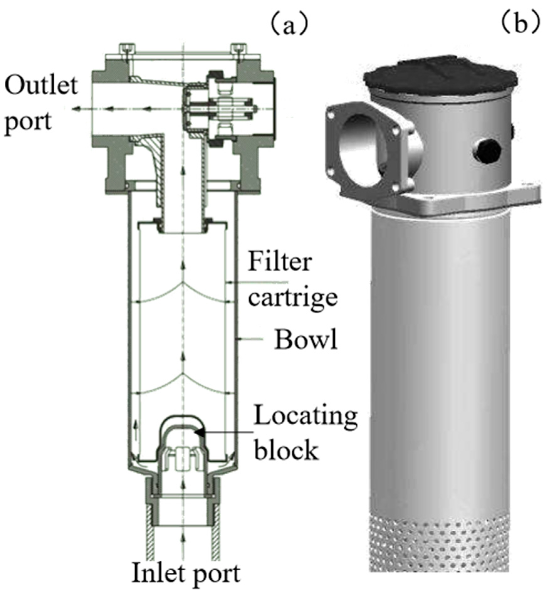
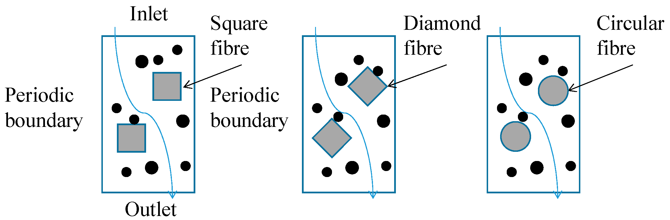
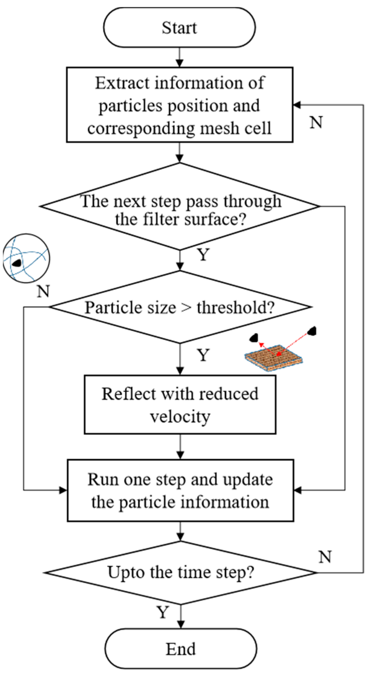
2.2. Filter Cartridge Modelling
3. Computational Settings
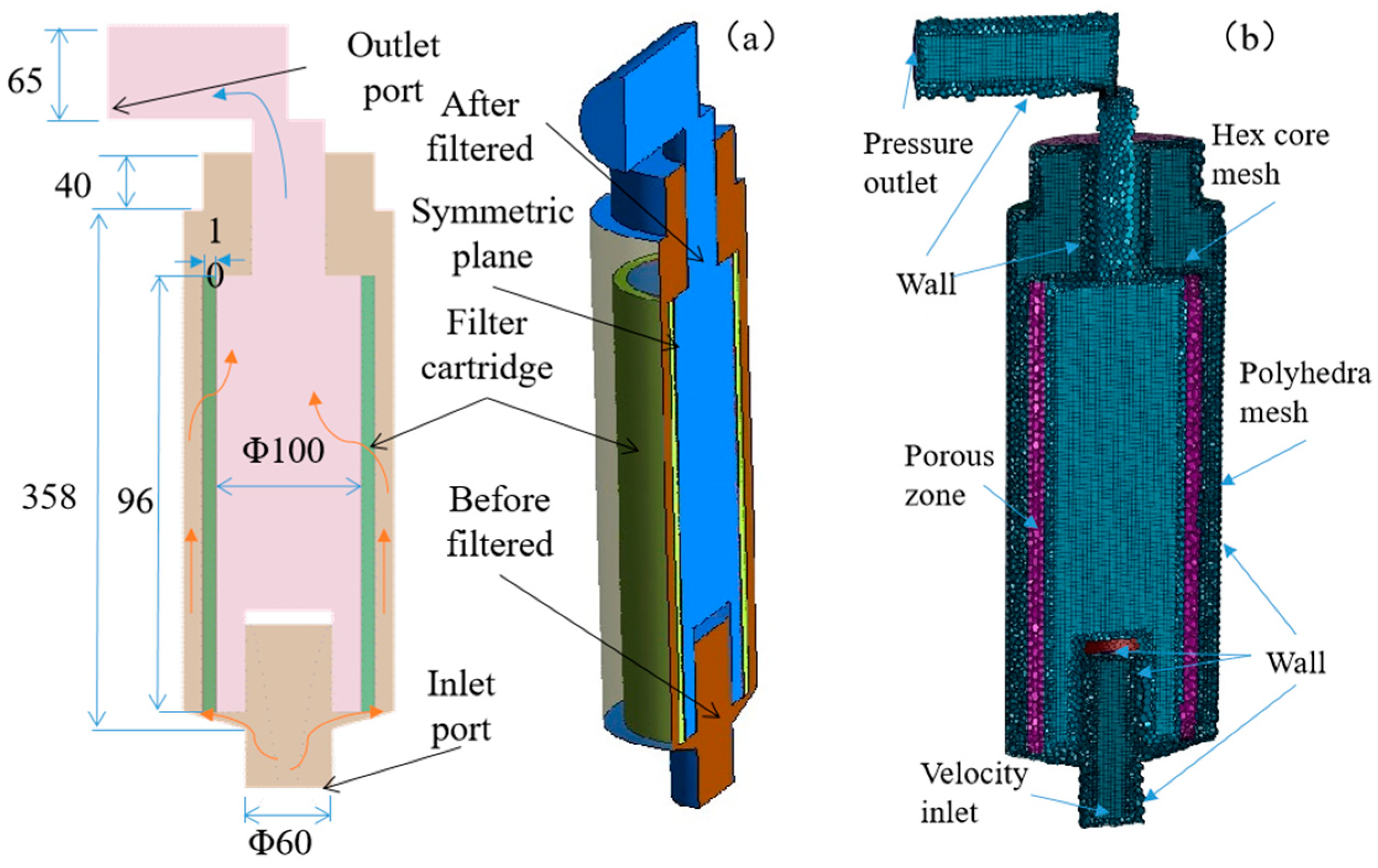
3.1. Geometry, Mesh, and Boundary Condition
3.2. Model Configurations and Parameters
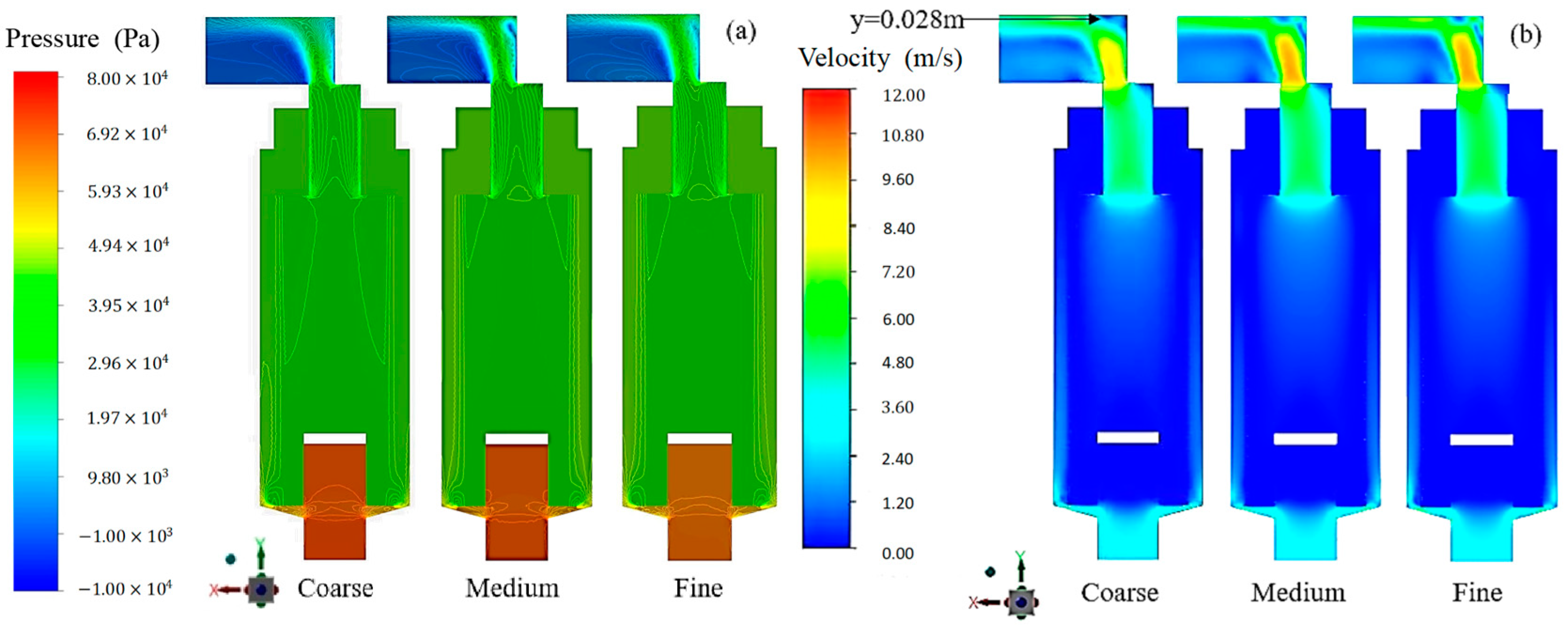
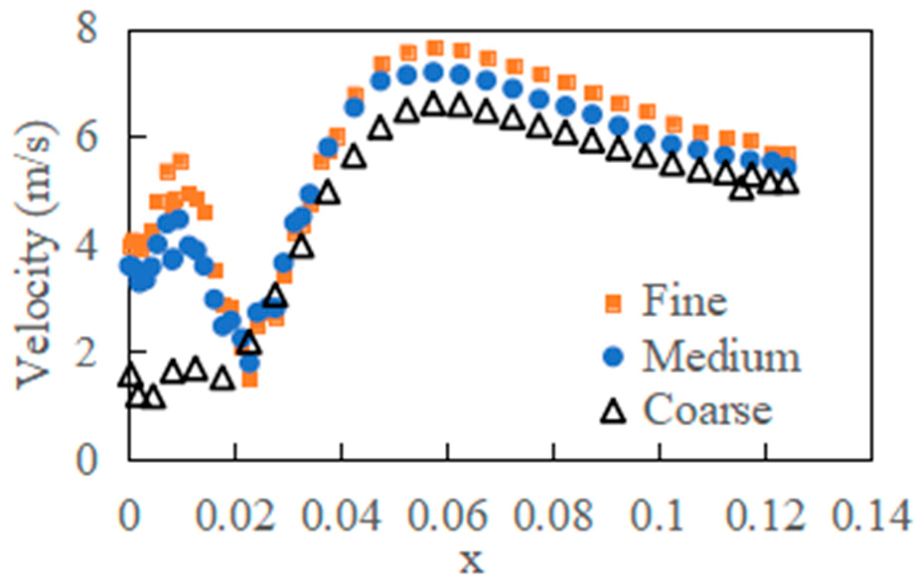
3.3. Sensitivity of Mesh Size
3.4. Model Verification
4. Discussion
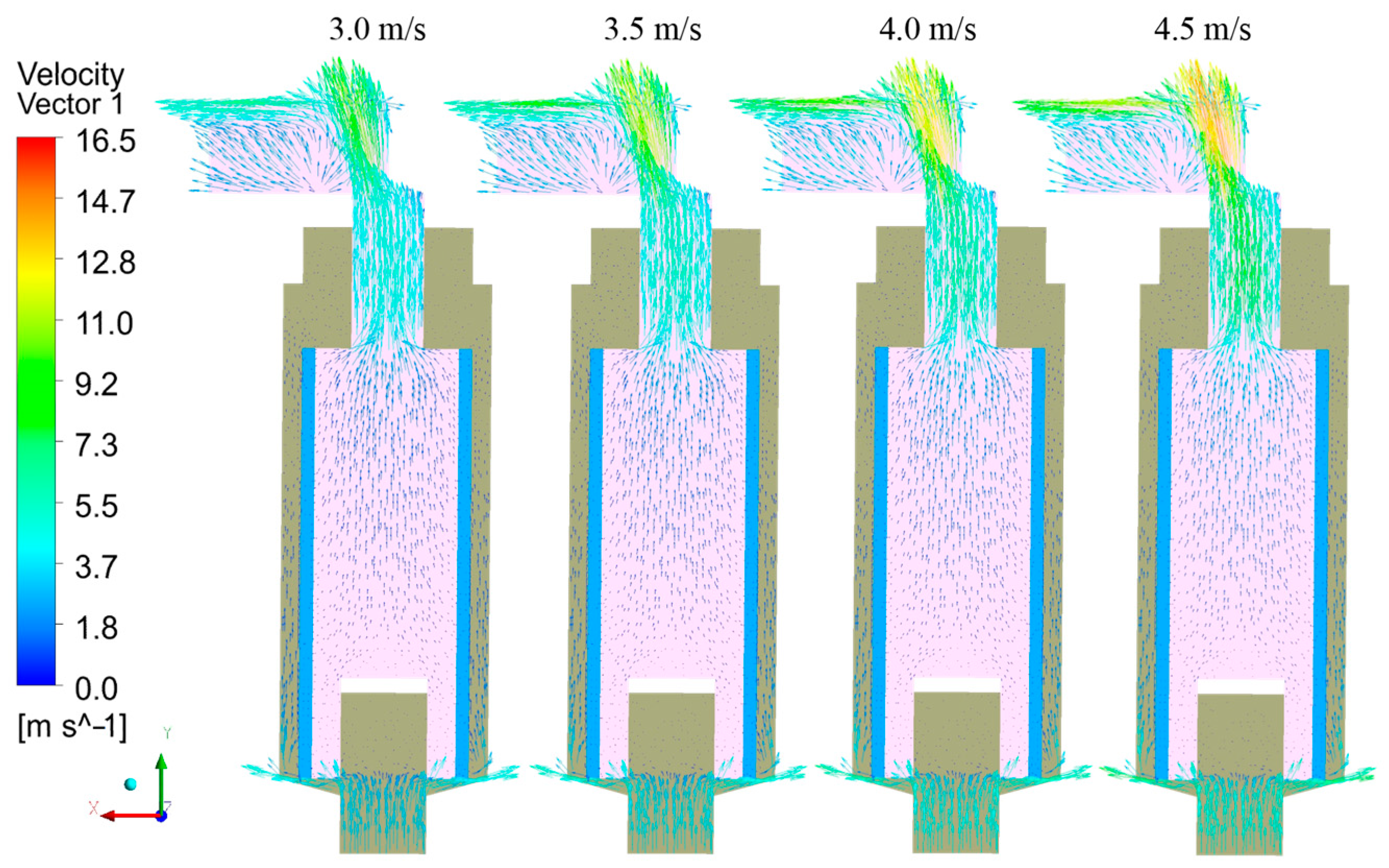
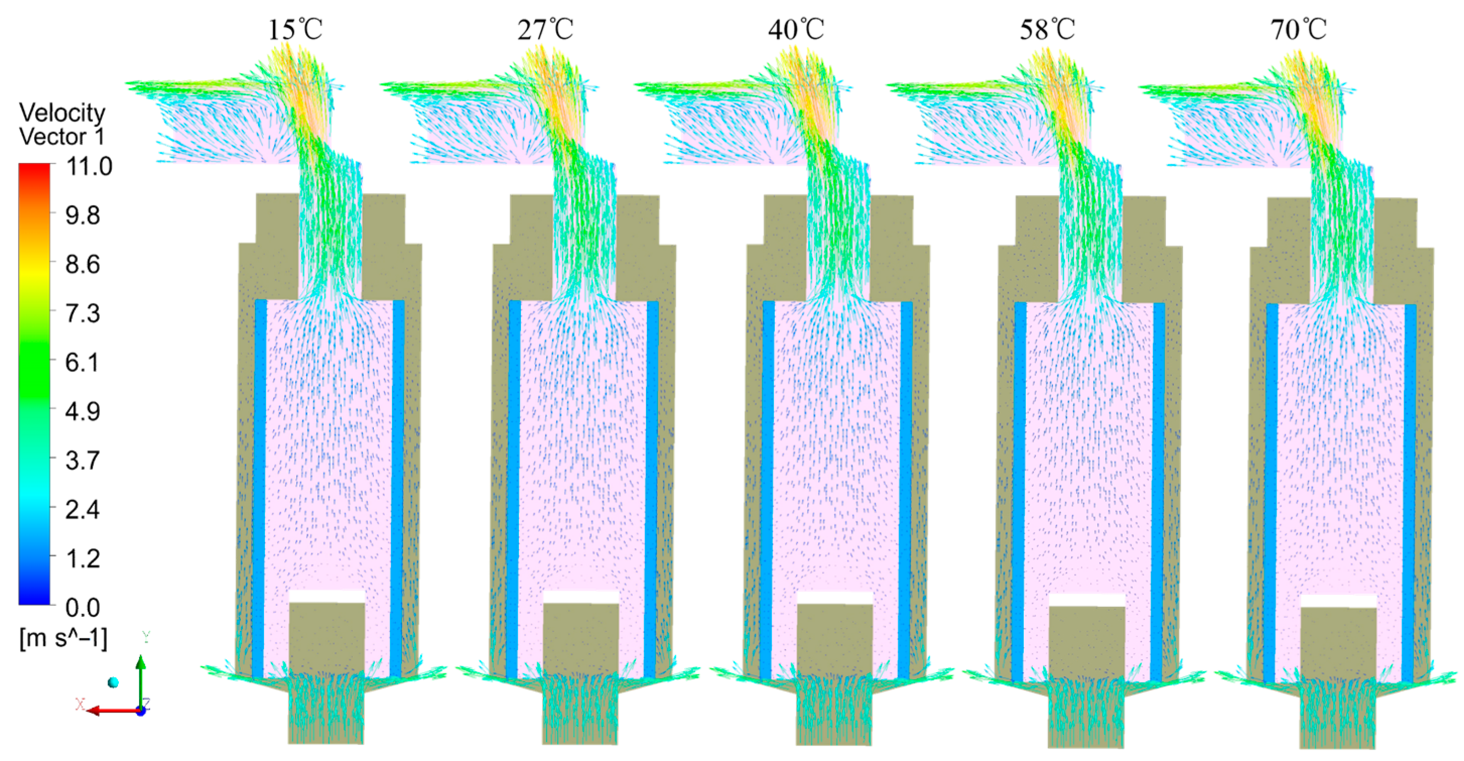
4.1. Velocity Vectors
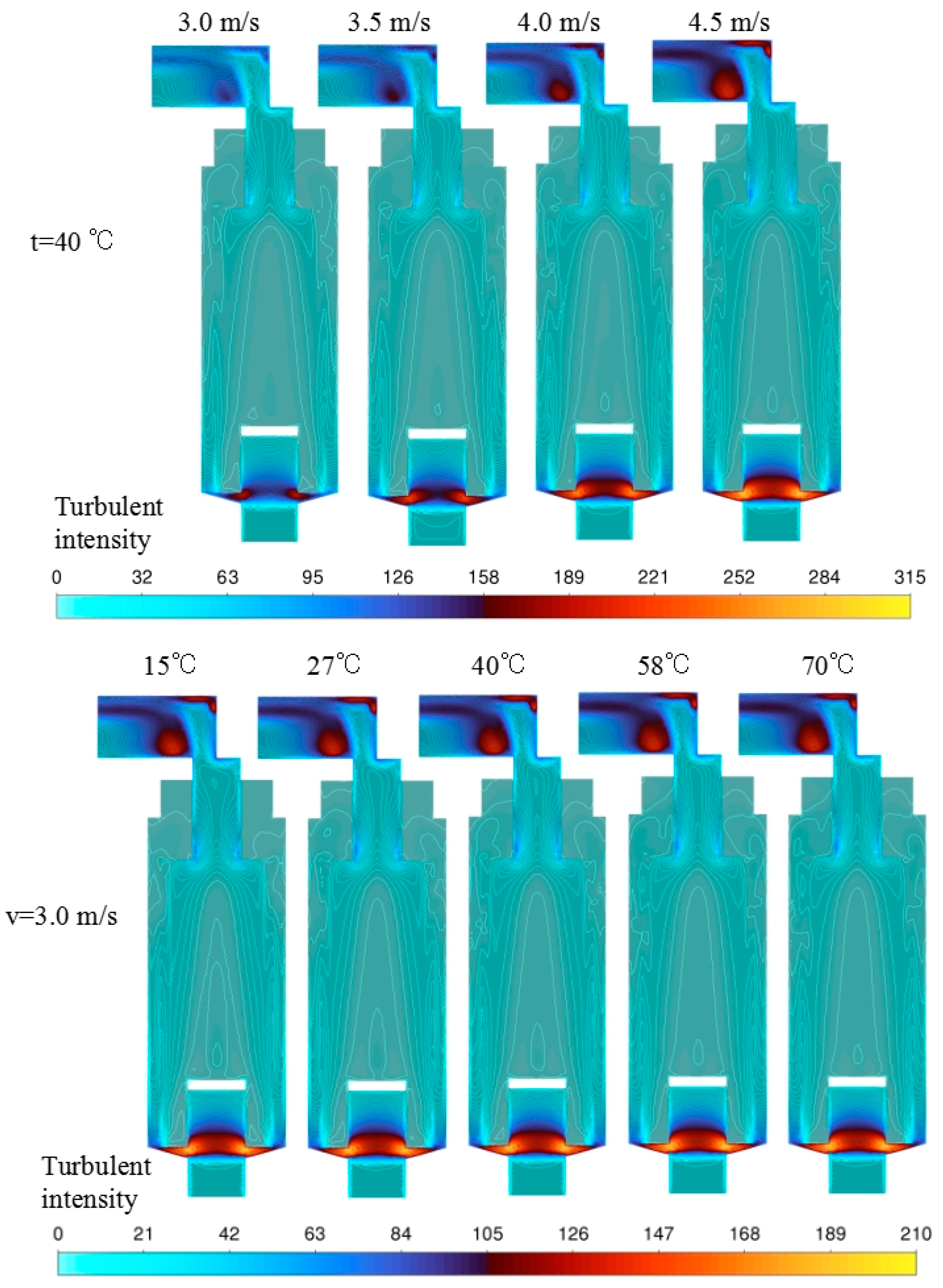
4.2. Turbulent Intensity
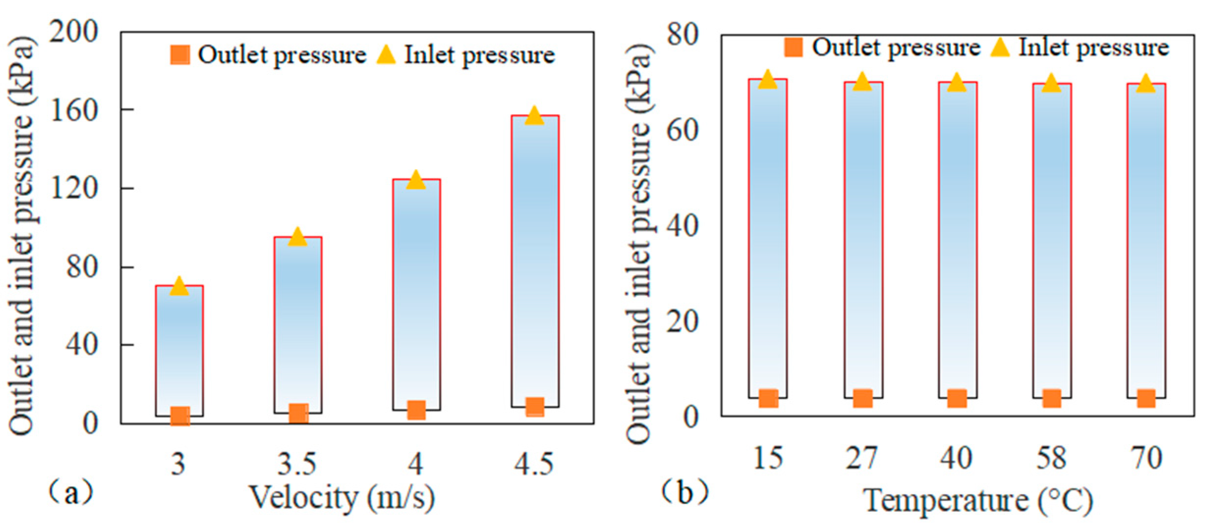
4.3. Pressure Loss
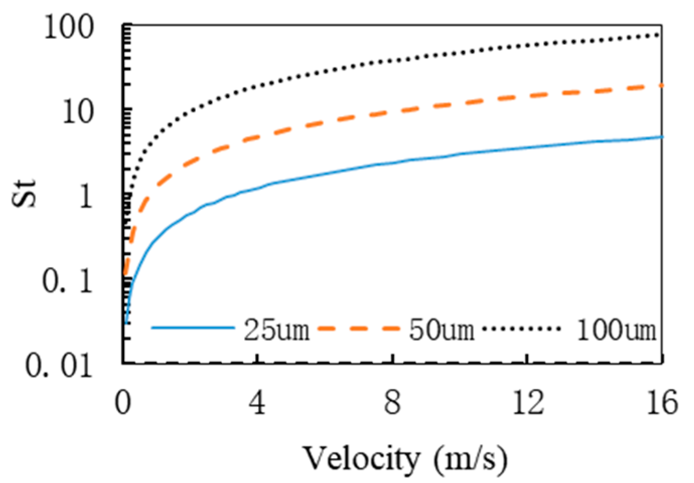
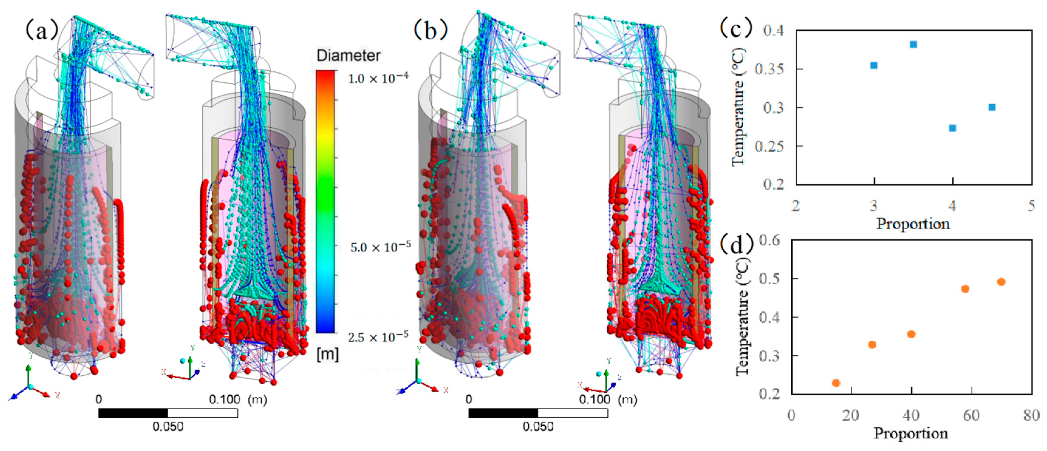
4.4. Particle Behavior
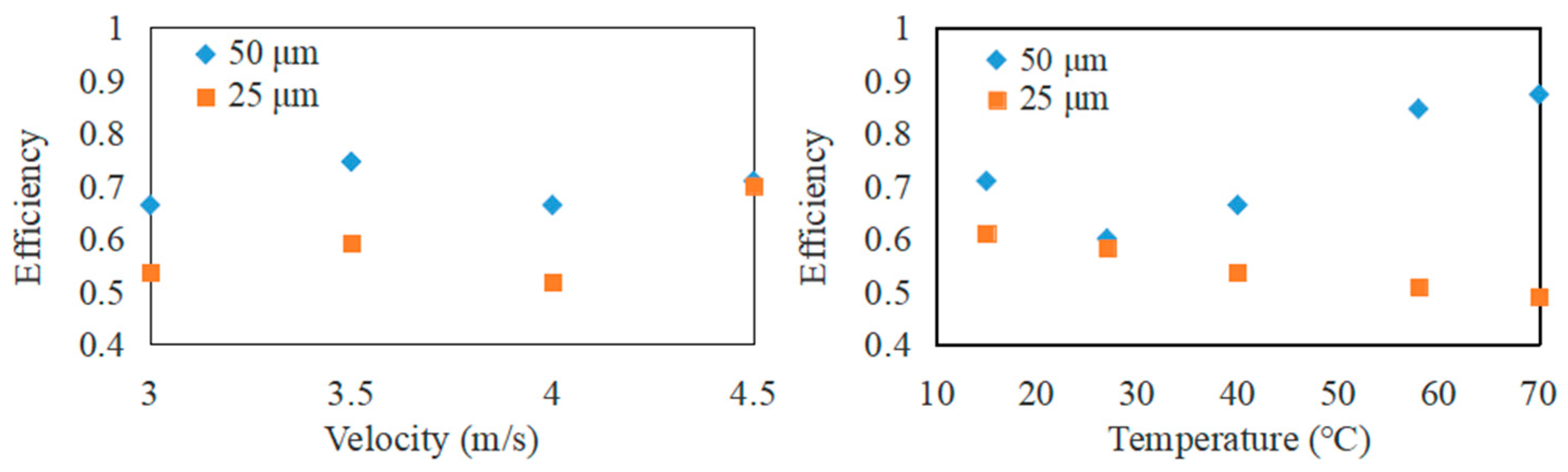
4.5. Filtering Efficiency
5. Conclusions
Author Contributions
Funding
Data Availability Statement
Acknowledgments
Conflicts of Interest
Abbreviations
| CFD | Computational Fluid Dynamics |
| DPM | Discrete Phase Model |
| DEM | Discrete Element Method |
| LBM | Lattice Boltzmann Method |
References
- Gorle, J.M.R.; Heiskanen, V.M.; Nissi, S.; Majas, M. Effect of temperature, flow rate and contamination on hydraulic filtration. MM Sci. J. 2018, 2018, 2490–2493. [Google Scholar] [CrossRef]
- Sun, D. Microscale study on dynamics of particles in slurry filtrated through porous media. Comput. Part. Mech. 2023, 11, 745–755. [Google Scholar] [CrossRef]
- Lauriola, K.; Gomez, M.; Meyer, R.; Son, F.; Slipchenko, M.; Roy, S. High speed particle image velocimetry and particle tracking methods in reactive and non-reactive flows. In Proceedings of the AIAA Scitech 2019 Forum, San Diego, CA, USA, 7–11 January 2019. [Google Scholar] [CrossRef]
- Canilho, H.; Santos, C.; Taborda, C.; Falorca, I.; Fael, C. Measurements of suspended ashes concentration in turbulent flow with acoustic doppler velocimeter. Flow Meas. Instrum. 2022, 87, 102207. [Google Scholar] [CrossRef]
- Jakobsen, B.; Merrison, J.; Iversen, J. Laboratory study of aerosol settling velocities using laser Doppler velocimetry. J. Aerosol Sci. 2019, 135, 58–71. [Google Scholar] [CrossRef]
- Kelbaliev, I.; Rzaev, G.; Rasulov, R.; Guseinova, V. Simulation of anomalous oil filtration in a porous bed. J. Eng. Phys. Thermophys. 2015, 88, 299–304. [Google Scholar] [CrossRef]
- Ansari, V.; Goharrizi, S.; Jafari, S.; Abolpour, B. Numerical study of solid particles motion and deposition in a filter with regular and irregular arrangement of blocks with using Lattice Boltzmann method. Comput. Fluids 2015, 108, 170–178. [Google Scholar] [CrossRef]
- Wang, H.; Zhao, H.; Wang, K.; He, Y.; Zheng, C. Simulation of filtration process for multi-fiber filter using the Lattice-Boltzmann two-phase flow model. J. Aerosol Sci. 2013, 66, 164–178. [Google Scholar] [CrossRef]
- Liu, Z.; Wang, P. Numerical investigation of viscous flow fields around multifiber filters. Aerosol Sci. Technol. 1996, 25, 375–391. [Google Scholar] [CrossRef]
- Li, W.; Shen, S.; Li, H. Study and optimization of the filtration performance of multi–fiber filter. Adv. Powder Technol. 2016, 27, 638–645. [Google Scholar] [CrossRef]
- Wang, L.Y.; Yong, W.F.; Liya, E.Y.; Chung, T.-S. Design of high efficiency PVDF-PEG hollow fibers for air filtration of ultrafine particles. J. Membr. Sci. 2017, 535, 342–349. [Google Scholar] [CrossRef]
- Fan, J. Numerical Study of Particle Transport and Deposition in Porous Media. Ph.D. Thesis, INSA de Rennes, Rennes, France, 2018. [Google Scholar]
- Lin, K.; Tao, H.; Lee, K. An early stage of aerosol particle transport in flows past periodic arrays of clear staggered obstructions: A computational study. Aerosol Sci. Technol. 2014, 48, 1299–1307. [Google Scholar] [CrossRef]
- Zhou, Y.; Chen, L.; Gong, Y.; Wang, S. Pore-scale simulations of particles migration and deposition in porous media using LBM-DEM coupling method. Processes 2021, 9, 465. [Google Scholar] [CrossRef]
- Cao, B.; Wang, S.; Dong, W.; Zhu, J.; Qian, F.; Lu, J.; Han, Y. Investigation of the filtration performance for fibrous media: Coupling of a semi-analytical model with CFD on Voronoi-based microstructure. Sep. Purif. Technol. 2020, 251, 117364. [Google Scholar] [CrossRef]
- Liu, X.; Ding, X.; Chen, C.; An, R.; Guo, W.; Zhang, W.; Wang, Y. Investigating the filtration behavior of metal fiber felt using CFD-DEM simulation. Eng. Appl. Comput. Fluid Mech. 2019, 13, 426–437. [Google Scholar] [CrossRef]
- Wang, N.; Chen, W.; Ning, G.; Ma, H. Numerical investigation of influence of structure and operating parameters on performance of vortex oil filter. In Proceedings of the CSAA/IET International Conference on Aircraft Utility Systems (AUS 2018), Guiyang, China, 19–22 June 2018; pp. 1150–1155. [Google Scholar]
- del Pozo, D.F.; Ahmad, A.; Rehman, U.; Verliefde, A.; Nopens, I. A novel CFD model to predict solids concentration and pressure drop in deep bed granular filtration. Sep. Purif. Technol. 2022, 295, 121232. [Google Scholar] [CrossRef]
- Bagherzadeh, A.; Darbandi, M.; Barezban, M.B. Numerical simulation of particle separation in a two-phase flow passing through a vortex-based air classifier using Eulerian–Lagrangian DDPM approach. Powder Technol. 2024, 445, 120036. [Google Scholar] [CrossRef]
- Wu, C.L.; Nandakumar, K.; Berrouk, A.S.; Kruggel-Emden, H. Enforcing mass conservation in DPM-CFD models of dense particulate flows. Chem. Eng. J. 2011, 174, 475–481. [Google Scholar] [CrossRef]
- Zheng, Q.J.; Yang, R.Y.; Zeng, Q.H.; Zhu, H.P.; Dong, K.J.; Yu, A.B. Interparticle forces and their effects in particulate systems. Powder Technol. 2024, 436, 119445. [Google Scholar] [CrossRef]
- ANSYS Fluent. Ansys Fluent Theory Guide; ANSYS Inc.: Canonsburg, PA, USA, 2022. [Google Scholar]
- Oyegbile, B.; Akdogan, G.; Karimi, M. Modelling the dynamics of granular particle interactions in a vortex reactor using a coupled DPM-KTGF model. S. Afr. J. Chem. Eng. 2020, 34, 31–46. [Google Scholar] [CrossRef]
- Ma, H.; Zhou, L.; Liu, Z.; Chen, M.; Xia, X.; Zhao, Y. A review of recent development for the CFD-DEM investigations of non-spherical particles. Powder Technol. 2022, 412, 117972. [Google Scholar] [CrossRef]
- Xu, D.; Shen, Y. A novel CFD-DEM-DPM modelling of fluid-particles-fines reacting flows. Chem. Eng. Sci. 2024, 292, 120014. [Google Scholar] [CrossRef]
- Chen, H.; Li, Y.; Xiong, Y.; Wei, H.; Saxén, H.; Yu, Y. Effect of particle holdup on bubble formation in suspension medium by VOF–DPM simulation. Granul. Matter 2022, 24, 120. [Google Scholar] [CrossRef]
- Kolev, N.I. Drag, lift, and virtual mass forces. In Multiphase Flow Dynamics 2; Springer: Berlin/Heidelberg, Germany, 2011. [Google Scholar] [CrossRef]
- Kang, S.; Lee, H.; Kim, C.; Chen, R.; Pui, Y. Modeling of fibrous filter media for ultrafine particle filtration. Sep. Purif. Technol. 2019, 209, 461–469. [Google Scholar] [CrossRef]
- Wang, D.; Fan, L.-S. Particle characterization and behavior relevant to fluidized bed combustion and gasification systems. In Fluidized Bed Technologies for Near-Zero Emission Combustion and Gasification; Scala, F., Ed.; Woodhead Publishing Series in Energy; Woodhead Publishing: Sawston, UK, 2013; pp. 42–76. [Google Scholar]
- Li, J.; Wang, P.; Zheng, X. Effects of the Saffman lift force on particle statistics and turbulence modulation in two-phase flow. Phys. Rev. Fluids 2024, 9, 034301. [Google Scholar] [CrossRef]
- Liu, J.; Liu, K.; Zhao, T.; Xu, Z. A Three-Dimensional Simulation of Particle Distribution in a Separator and Structure Optimization with the Statistical Approach of Taguchi Method. Math. Probl. Eng. 2018, 2018, 7439245. [Google Scholar] [CrossRef]
- Belhaj, H.A.; Agha, K.R.; Nouri, A.M.; Butt, S.D.; Vaziri, H.H.; Islam, M.R. Numerical modeling of Forchheimer’s equation to describe Darcy and non-Darcy flow in porous media. In Proceedings of the SPE Asia Pacific Oil and Gas Conference and Exhibition, Jakarta, Indonesia, 9–11 September 2003; p. SPE-80440-MS. [Google Scholar]
- Hsu, C.T.; Cheng, P. The Brinkman model for natural convection about a semi-infinite vertical flat plate in a porous medium. Int. J. Heat Mass Transf. 1985, 28, 683–697. [Google Scholar] [CrossRef]
- ISO 3448:1992; Industrial Liquid Lubricants—ISO Viscosity Classification. International Organization for Standardization: Geneva, Switzerland, 1992.
- Donaldson. Hydraulic Filtration Product Guide. 2019. Available online: https://www.donaldson.com/content/dam/donaldson/engine-hydraulics-bulk/catalogs/Hydraulic/North-America/F112100-ENG/Hydraulic-Filtration-Product-Guide.pdf (accessed on 15 January 2023).
- Lam, W.H.; Robinson, D.J.; Hamill, G.A.; Johnston, H.T. An effective method for comparing the turbulence intensity from LDA measurements and CFD predictions within a ship propeller jet. Ocean Eng. 2012, 52, 105–124. [Google Scholar] [CrossRef]
- Li, D.; Zhao, Z.; Li, Y.; Wang, Q.; Li, R.; Li, Y. Effects of the particle Stokes number on wind turbine airfoil erosion. Appl. Math. Mech. 2018, 39, 639–652. [Google Scholar] [CrossRef]


| Parameters | Value | |
|---|---|---|
| Porous medium model | Permeability of the porous medium (m2) | 1/20,011,000 |
| Inertial resistance factor (m−1) | 9 × 10⁴ | |
| Threshold size (μm) | 60 | |
| Discrete Phase Model | Injected particle diameters (μm) | 25, 50, 100 |
| Injected rate for 100 μm (kg/s) | 4 × 10⁻⁶ | |
| Injected rate for 50 μm (kg/s) | 1.6 × 10⁻⁷ | |
| Injected rate for 25 μm (kg/s) | 2 × 10⁻⁸ | |
| Particle injection stop time (s) | 0.5 | |
| Contact model | Spring–Dashpot | |
| Elastic coefficient (N/m) | 10 | |
| Dashpot coefficient | 0.6 | |
| Velocity (m/s) | 2 | |
| Virtual mass factor | 0.5 | |
| Normal reducing coefficient | 0.05 | |
| Tangential reducing coefficient | 0.1 | |
| Hydraulic oil | Density (kg/m3) | 830 |
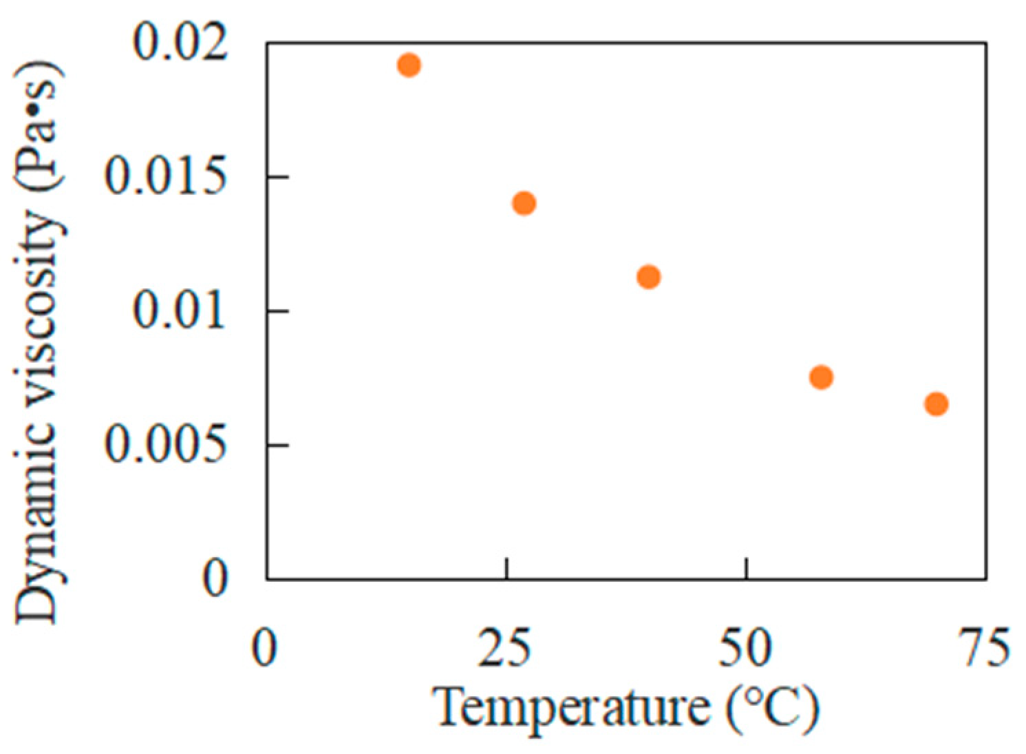
| Viscosity (kg/m/s) | Figure 5 | |
| Particle contamination | Density (kg/m3) | 2550 |
| Boundary | Inlet oil velocity (m/s) | 3.0, 3.5, 4.0, 4.5 |
| Initial outlet pressure (MPa) | 0 | |
| Temperature (℃) | 15, 27, 40, 58, 70 | |
| Timestep size (s) | 0.01 | |
| Calculation time (s) | 1.8 | |
| Algorithm | Pressure–Velocity Coupling | |
|---|---|---|
| Discretization | Pressure | Second order |
| Momentum | First order upwind | |
| Turbulent kinetic energy | First order upwind | |
| Turbulent dissipation rate | First order upwind | |
| Explicit relaxation factor | Momentum | 0.75 |
| Pressure | 0.75 | |
| Coarse | Medium | Fine | |
|---|---|---|---|
| Number of cells | 45,039 | 189,253 | 586,483 |
| Number of nodes | 158,708 | 525,875 | 1,291,387 |
| Minimum cell length | 0.5 | 0.3 | 0.2 |
| Maximum cell length | 4 | 2.4 | 1.6 |
Disclaimer/Publisher’s Note: The statements, opinions and data contained in all publications are solely those of the individual author(s) and contributor(s) and not of MDPI and/or the editor(s). MDPI and/or the editor(s) disclaim responsibility for any injury to people or property resulting from any ideas, methods, instructions or products referred to in the content. |
© 2025 by the authors. Licensee MDPI, Basel, Switzerland. This article is an open access article distributed under the terms and conditions of the Creative Commons Attribution (CC BY) license (https://creativecommons.org/licenses/by/4.0/).
Share and Cite
Chen, J.; Xi, D.; Wang, G.; Zhou, M.; Hu, Y.; Xie, X. Numerical Investigation into Particle Migration Characteristics in Hydraulic Oil Filtration. Processes 2025, 13, 1289. https://doi.org/10.3390/pr13051289
Chen J, Xi D, Wang G, Zhou M, Hu Y, Xie X. Numerical Investigation into Particle Migration Characteristics in Hydraulic Oil Filtration. Processes. 2025; 13(5):1289. https://doi.org/10.3390/pr13051289
Chicago/Turabian StyleChen, Jian, Dongyang Xi, Guichao Wang, Mi Zhou, Yibo Hu, and Xihua Xie. 2025. "Numerical Investigation into Particle Migration Characteristics in Hydraulic Oil Filtration" Processes 13, no. 5: 1289. https://doi.org/10.3390/pr13051289
APA StyleChen, J., Xi, D., Wang, G., Zhou, M., Hu, Y., & Xie, X. (2025). Numerical Investigation into Particle Migration Characteristics in Hydraulic Oil Filtration. Processes, 13(5), 1289. https://doi.org/10.3390/pr13051289