Trajectory-Integrated Kriging Prediction of Static Formation Temperature for Ultra-Deep Well Drilling

Abstract

The accurate prediction of static formation temperature (SFT) is essential for ensuring safety and efficiency in ultra-deep well drilling operations. Excessive downhole temperatures (>150 °C) can degrade drilling fluids, damage temperature-sensitive tools, and pose serious operational risks. Conventional methods for SFT determination—including direct measurement, temperature recovery inversion, and artificial intelligence models—are often limited by post-drilling data dependency, insufficient spatial resolution, high computational costs, or a lack of adaptability to complex wellbore geometries. In this study, we propose a new pseudo-3D Kriging interpolation framework that explicitly incorporates real wellbore trajectories to improve the spatial accuracy and applicability of pre-drilling SFT predictions. By systematically optimizing key hyperparameters (θ = [10, 10], lob = [0.1, 0.1], upb = [20, 200]) and applying a grid resolution of 100 × 100, the model demonstrates high predictive fidelity. Validation using over 5.1 million temperature data points from 113 wells in the Shunbei Oilfield reveals a relative error consistently below 5% and spatial interpolation deviations within 5 °C. The proposed approach enables high-resolution, trajectory-integrated SFT forecasting before drilling with practical computational requirements, thereby supporting proactive thermal risk mitigation and significantly enhancing operational decision-making on ultra-deep wells.

1. Introduction

As the exploration and development of oil and gas resources advance, the focus has increasingly shifted toward drilling in deep and ultra-deep reservoirs [1,2]. During the drilling process, the circulation of drilling fluid causes it to continuously absorb heat from the surrounding formation, leading to a rise in the temperature of the drilling fluid within the wellbore. Therefore, as the well depth increases, SFT rises, and the drilling fluid temperature subsequently becomes elevated. The elevated temperature of drilling fluid can lead to numerous issues, including the degradation of the drilling fluid, the failure of drill pipes, and malfunctions of downhole instruments, as their temperature tolerance limits (typically around 150 °C [3,4]) are often exceeded. High temperatures can also complicate signal transmission and pose other operational challenges [5,6]. Therefore, it is crucial to accurately predict the SFT initially, to precisely forecast the drilling fluid temperature within the wellbore, and then manage it effectively. Accurately predicting the SFT can significantly enhance the speed and safety of well drilling operations.

To accurately determine SFT, researchers have identified four primary methods: (1) SFT measurement using downhole instruments, (2) SFT inversion based on drilling fluid temperature recovery data, (3) SFT inversion based on the difference between mechanistic model predictions and drilling fluid temperature measurements, and (4) SFT prediction based on artificial intelligence (AI) models. The first method directly measures SFT using instruments placed downhole. However, to ensure the recorded temperature reflects SFT, drilling fluid circulation must be halted for an extended time, which is usually 2 to 4 days [7], allowing the drilling fluid temperature to be close to the SFT. In addition, as the well depth increases, drilling fluid temperature, either during circulation or when circulation is halted, may exceed the temperature tolerance limits of the measuring instruments. The second method is inverting SFT using the recovery data of drilling fluid temperature after fluid circulation is stopped. The SFT estimations can be derived from seven analytical methods [8] according to variations in heat source characteristics and heat transfer modes: the Horner method [9], the Brennand method [10], the Kutasov–Eppelbaum method [11], the Leblanc method [12], the Manetti method [13], the spherical–radial heat flow method [14], and the conductive–convective cylindrical source method [15]. Some scholars have utilized an artificial neural network to estimate SFT using bottomhole temperature (BHT) measurements, shut-in time, and transient temperature gradient as input data [16]. The limitation of this method is that it requires temperature recovery data at various times from a specific depth, but in practice, it is rare to have multiple data points that track temperature changes over time at the same depth in the field. In addition, its accuracy significantly deteriorates when applied to complex well structures (e.g., horizontal wells and extended-reach wells), as the analytical models are primarily designed for vertical wells. Researchers have proposed a third methodology to overcome the requirement of measuring multiple temperature points over time at a single location in the second approach. This improved method requires only a single temperature measurement at a single depth location, which is then coupled with a wellbore temperature field model to determine SFT inversely through data–model integration. As for the third method, some researchers analyze heat transfer laws and establish prediction models for the SFT. Some scholars have utilized a proportional–integral control method [17] combined with inverse heat transfer analysis to dynamically adjust formation parameters based on a single logged temperature measurement for SFT inversion. Other researchers have established numerical heat transfer models [18] to solve transient heat transfer equations with post-shut-in wellbore temperatures as initial conditions, tracking temperature recovery until thermal equilibrium is reached for SFT determination. Furthermore, AI [8] has been applied to predict wellbore parameters and enable efficient SFT inversion based on these parameters. However, this method relies on the inversion of SFT based on the measured drilling fluid temperature during the drilling process, which inherently prevents its application for pre-drilling predictions. Moreover, it generally yields an averaged geothermal gradient from the surface to the bottomhole, rather than providing detailed temperature distribution characteristics. The fourth method involves predicting SFT based on AI models [19,20,21,22,23,24,25,26]. The methodology for AI-driven SFT prediction entails the following key procedures: comprehensive petrophysical data collection and systematic preprocessing are first implemented to ensure the integrity of the dataset. Multiple machine learning models are subsequently constructed through rigorous algorithm selection and hyperparameter optimization. These models undergo quantitative evaluation using domain-specific metrics, including mean absolute error and coefficient of determination, supplemented by geothermal gradient validation protocols. Interpretability analysis utilizes SHAP values to quantify the contributions of variables to SFT estimation. Finally, an ensemble prediction framework integrates optimized base models to achieve enhanced SFT inversion accuracy through the weighted aggregation of multi-model outputs. However, this method involves cumbersome operational procedures and requires computationally intensive processing, resulting in prolonged execution time. Each of these methods has its advantages and limitations, emphasizing the need for further refinement to achieve both rapid and accurate predictions of SFT.

Currently, an efficient and accurate method for predicting SFT in new wells is lacking. Kriging interpolation is a geostatistical method that predicts attribute values at unknown locations based on known data points and their spatial relationships. This method demonstrates high computational efficiency while maintaining superior prediction accuracy. Thus, Kriging interpolation emerges as a practical method for predicting SFT. This geostatistical technique enables the prediction of unknown values by interpolating from known points, taking into account the spatial relationships between these points and the target location. Over the years, Kriging interpolation has evolved into various forms, including ordinary Kriging and universal Kriging, and is extensively applied across multiple domains. For instance, the Kriging interpolation method has been utilized in meteorological forecasting and civil engineering applications. Falah et al. [27] combined an expanded spatial Durbin model with ordinary Kriging to forecast the rainfall patterns in Java Island, whose mean absolute percentage error reached 1.956%. Shanmugam et al. [28] used ordinary Kriging for spatial interpolation of LiDAR point cloud data to fill in data voids, thereby enabling a more accurate assessment of scour conditions surrounding bridges. In Earth sciences, Kriging interpolation is commonly used in geothermal fields. Gu et al. [29] combined laboratory measurements and seismic data, utilizing the external drift kriging method to improve the interpolation of thermal conductivity, thereby enhancing the accuracy of thermal conductivity estimates. Jeong et al. [30] developed a hybrid model that combines the finite element method and the Kriging method to accurately estimate the undisturbed ground temperature, achieving an average mean absolute percentage error of 3.67%. Che and Jia [31] constructed a three-dimensional geological model of coal seams using the weighted Kriging method and validated the model’s accuracy based on the collected data from 259 boreholes. Su et al. [32] constructed a 3D temperature field model and employed the Kriging interpolation method to spatially predict the temperature field during the underground coal gasification process. Agemar et al. [33] used Kriging interpolation technology to integrate data from over 10,500 wells and more than 700 surface datasets, creating a more consistent temperature model and effectively handling variations in data density and quality. Similarly, Sepúlveda et al. [34] verified the temperature and stratigraphic data of more than 200 boreholes using the Kriging interpolation method. Through standardization processing, they enhanced the data’s usability, pinpointed the key geological factors influencing temperature and strata, and highlighted the complex relationship between strata and temperature. It was found that deep-seated structures have a significant influence on temperature distribution and that temperature changes exhibit obvious anisotropic characteristics.

Although previous studies have conducted Kriging interpolation predictions for SFT, such applications have predominantly focused on geothermal resource assessment. Geothermal wells, characterized by relatively shallower depths and simpler well structures compared to oil and gas wells, demonstrate distinct engineering features that differentiate them from conventional hydrocarbon wells. Therefore, this paper proposes a novel pseudo-3D method for predicting SFT based on Kriging interpolation that takes into account the actual wellbore trajectory. By considering the variations in wellbore trajectories, this method enables more accurate predictions of SFT before drilling commences. This approach not only retains the capability of traditional 2D kriging to rapidly interpolate planar SFT distributions from sparse data points, but also enables the visualization of SFT distribution across stratigraphic profiles. With the new method, the prediction of SFT can be made correctly and efficiently. Implementing appropriate cooling measures based on SFT-derived wellbore temperature calculations during drilling operations, as illustrated in Figure 1, enhances safety throughout the drilling process.

2. Methodology

In this study, SFTs were predicted using the ordinary Kriging interpolation method. Section 2.1 outlines the theoretical foundation and implementation of the ordinary Kriging algorithm for SFT prediction. Section 2.2 describes the structure and key characteristics of the SFT dataset used in this study. Section 2.3 details the preprocessing procedures required for interpolation, including wellbore trajectory reconstruction and true vertical depth (TVD) alignment. Finally, Section 2.4 introduces the statistical metrics used to evaluate the prediction accuracy and model performance.

2.1. Ordinary Kriging for SFT Prediction

Ordinary Kriging (OK) is an optimal and unbiased spatial interpolation technique that utilizes spatial autocorrelation to estimate values at unsampled locations. This section provides a detailed mathematical formulation of the OK framework, emphasizing its underlying assumptions and step-by-step implementation procedure.

OK assumes that the spatial process $Z\left(s\right)$ satisfies second-order stationarity; that is, the expectation $E\left[Z\left(s\right)\right]=\mu$ is constant, and the covariance depends only on the spatial lag $h$: $\mathrm{C}\mathrm{o}\mathrm{v}\left(Z\left(s\right),Z\left(s+h\right)\right)=C\left(h\right)$. Under this assumption, the predicted value $\widehat{Z}\left(s_0\right)$ at an unobserved location $s_0$ is estimated by a linear weighted sum of observed values at known locations ${\left\{s_i\right\}}_{i=1}^n$

$$\widehat{Z}\left(s_0\right)={\displaystyle \sum _{i=1}^n{\lambda }_{i}Z\left(s_i\right)}$$

(1)

where ${\lambda }_i$ are weight coefficients. To ensure the unbiasedness of the predictions—that is, to make the expected value of the prediction error zero—the sum of the Kriging weights must equal one

$${\displaystyle \sum _{i=1}^n{\lambda }_i=1}$$

(2)

The variance of the prediction error is expressed as

$$\mathrm{Var}\left(\widehat{Z}\left(s_0\right)-Z\left(s_0\right)\right)={\displaystyle \sum _{i=1}^n{\displaystyle \sum _{j=1}^n{\lambda }_i{\lambda }_{j}C\left(s_i-s_j\right)+C\left(0\right)}}-2{\displaystyle \sum _{i=1}^n{\lambda }_{i}C\left(s_i-s_0\right)}$$

(3)

where $C\left(h\right)$ is the covariance function, and $C\left(0\right)=\mathrm{V}\mathrm{a}\mathrm{r}\left(Z\right(s\left)\right)$. Minimizing this variance is the core objective of Kriging.

Introducing a Lagrangian multiplier ${\varphi }_l$, the objective function is constructed as

$$L={\displaystyle \sum _{i=1}^n{\displaystyle \sum _{j=1}^n{\lambda }_i{\lambda }_{j}C\left(s_i-s_j\right)}}-2{\displaystyle \sum _{i=1}^n{\lambda }_{i}C\left(s_i-s_0\right)}+2{\varphi }_l\left({\displaystyle \sum _{i=1}^n{\lambda }_i-1}\right)$$

(4)

Taking partial derivatives with respect to ${\lambda }_k$ and ${\varphi }_l$, and setting them to zero yields the following:

Weight equations

$${\displaystyle \sum _{j=1}^n{\lambda }_{j}C\left(s_k-s_j\right)+{\varphi }_l=C}\left(s_k-s_0\right),k=1,2,\cdots ,n$$

(5)

Write the equations in matrix form

$$\left[\begin{array}{cccc}C\left(s_1-s_1\right)& \cdots & C\left(s_1-s_n\right)& 1\\ ⋮& \ddots & ⋮& ⋮\\ C\left(s_n-s_1\right)& \cdots & C\left(s_n-s_n\right)& 1\\ 1& \cdots & 1& 0\end{array}\right]\left[\begin{array}{c}{\lambda }_1\\ ⋮\\ {\lambda }_n\\ {\varphi }_l\end{array}\right]=\left[\begin{array}{c}C\left(s_1-s_0\right)\\ ⋮\\ C\left(s_n-s_0\right)\\ 1\end{array}\right]$$

(6)

Solving this linear system provides the optimal weights ${\lambda }_i$ and the multiplier ${\varphi }_l$.

In practice, the semi-variogram $\gamma \left(h\right)=C\left(0\right)-C\left(h\right)$ is often used instead of the covariance function. The system then becomes

$$\left\{\begin{array}{l}{\displaystyle \sum _{j=1}^n{\lambda }_j\gamma \left(s_k-s_j\right)-{\varphi }_l=\gamma }\left(s_k-s_0\right),k=1,2,\cdots ,n\\ {\displaystyle \sum _{i=1}^n{\lambda }_i=1}\end{array}\right.$$

(7)

With the corresponding matrix form

$$\left[\begin{array}{cccc}\gamma \left(s_1-s_1\right)& \cdots & \gamma \left(s_1-s_n\right)& 1\\ ⋮& \ddots & ⋮& ⋮\\ \gamma \left(s_n-s_1\right)& \cdots & \gamma \left(s_n-s_n\right)& 1\\ 1& \cdots & 1& 0\end{array}\right]\left[\begin{array}{c}{\lambda }_1\\ ⋮\\ {\lambda }_n\\ {\varphi }_l\end{array}\right]=\left[\begin{array}{c}\gamma \left(s_1-s_0\right)\\ ⋮\\ \gamma \left(s_n-s_0\right)\\ 1\end{array}\right]$$

(8)

The prediction Kriging variance is calculated as

$${\sigma }_{\mathrm{OK}}^2={\displaystyle \sum _{i=1}^n{\lambda }_i\gamma \left(s_i-s_0\right)}+{\varphi }_l$$

(9)

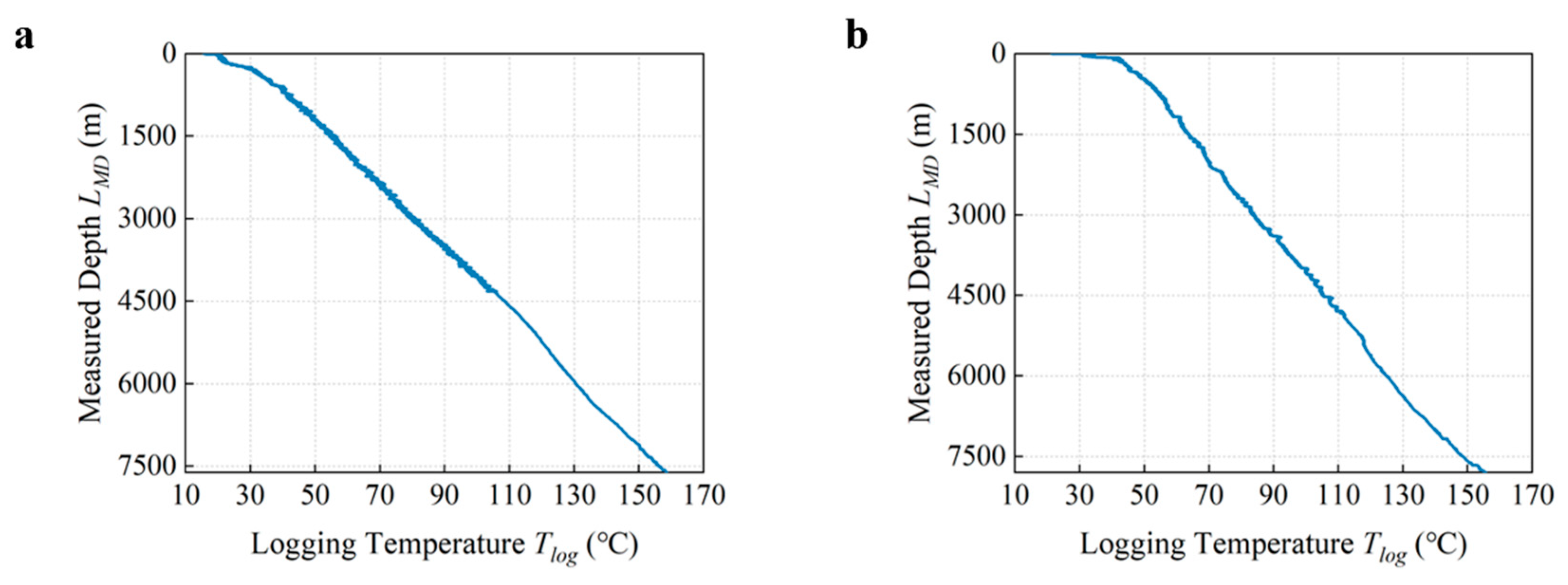
2.2. Description of SFT Data

The SFT data used in this study were exclusively derived from well-logging temperature measurements collected from completed wells in the Shunbei Oilfield. Well-logging temperature data represents the closest approximation to SFT. Acquired through direct measurement of formations, this temperature reflects the collective influence of geological properties including terrestrial heat flow, geological structures, and lithology. Therefore, utilizing well log temperature data as the primary source for SFT enables models to inherently account for these multifaceted geological factors without the need for their separate analysis. The dataset comprises measurements from 113 wells, predominantly directional and horizontal wells, distributed across five different fault zones. These wells cover an area of approximately 230 $\mathrm{k}\mathrm{m}$ $\times$ 170 $\mathrm{k}\mathrm{m}$, extending vertically to depths of up to 9 $\mathrm{k}\mathrm{m}$ (as shown in Figure 2).

As shown in

Table 1. Typical characteristics of temperature logging data from 113 wells in the Shunbei Oilfield.

Fault Zone	Well Number	SFT Data Point Number	$\mathbf{Max}. \mathbf{MD} (\mathbf{m}$)	$\mathbf{Min}. \mathbf{MD} (\mathbf{m}$)	$\mathbf{Max}. \mathbf{TVD} (\mathbf{m}$)	$\mathbf{Min}. \mathbf{TVD} (\mathbf{m}$)	Max. SFT (°C)	Min. SFT (°C)
#1	34	1,379,981	8750.13	7271.00	8240.70	7270.72	163.89	139.54
#2	26	1,237,893	8996.75	6977.63	8434.68	6977.63	180.79	138.29
#3	29	1,284,782	8799.00	7364.05	8223.88	7364.05	178.72	134.95
#4	8	385,669	8959.38	7679.50	8473.30	7679.50	180.19	155.37
#5	16	881,914	9272.50	8049.05	8915.93	7863.50	199.06	164.43
Total	113	5,170,239	9272.50	6977.63	8915.93	6977.63	199.06	134.95

and Figure 3, the 113 wells in the Shunbei Oilfield exhibit measured depths (MDs) predominantly ranging from 7000 m to 9000 m, with TVDs mostly falling within the same interval. BHTs generally range from approximately 135 °C to 200 °C across all fault zones. Table 1 summarizes the key characteristics of temperature logging data for each of the five fault zones. Among them, fault zone #5 contains the wells with the greatest MD (9272.50 m) and the highest recorded SFT (199.06 °C), while fault zone #2 includes the well with the shallowest MD (6977.63 m). In total, the dataset comprises more than 5.1 million SFT data points. Figure 3 displays the distribution of SFT values for each fault zone using box plots. The gray boxes indicate the interquartile range (IQR), covering the middle 50% of the data (i.e., 25% to 75%), and the whiskers extend to 1.5 times the IQR, typically encompassing the entire range of observed temperatures. This visual representation highlights the spatial heterogeneity of SFT distributions across different structural zones, reflecting both localized thermal anomalies and regional geothermal gradients within the study area.

The SFT was originally measured at discrete points with an MD interval of 0.125 $\mathrm{m}$. To enable the practical application of Kriging interpolation, the data were resampled to a uniform spacing of 1 $\mathrm{m}$ along TVD, thereby achieving a vertical resolution of 1 $\mathrm{m}$. In contrast, the horizontal resolution remains relatively coarse due to the wide spacing between wells. Given the optimal drainage area required for oil and gas production, the horizontal distance between wells typically ranges from several hundred meters to several kilometers, which limits the lateral spatial density of the temperature dataset.

2.3. Preprocessing of SFT Data

The SFT data described in the previous section were typically recorded at uniform intervals along the MD, which renders them unsuitable for direct application in the Kriging interpolation model that operates on TVD. Therefore, data preprocessing is necessary to convert the dataset into a format compatible with interpolation.

First, significant seasonal variations in surface temperature at the well sites introduce thermal fluctuations in the shallow formation near the wellhead. For instance, surface formation temperatures can fall below 0 °C in winter and rise above 50 °C in summer. These fluctuations result in non-representative temperature measurements in shallow intervals, which can introduce seasonal bias into the interpolation model. Among all well-logging temperature datasets, the majority are acquired on a section-by-section basis during drilling operations. However, a limited number of wells possess continuous temperature logs covering the entire wellbore. Figure 4 presents the full-borehole temperature logs from two such wells from different fault zones. These data reveal that surface temperature effects typically diminish beyond depths of 200 m to 500 m. Section-based temperature measurements generally commence with the second spud-in section, which typically commences below depths of 500 m. Consequently, the temperature data acquired from these section-based measurements are inherently free from surface temperature effects.

Second, the SFT logging data were collected over multiple logging runs during the drilling process. Due to differences in logging conditions and instrument calibration across runs, temperatures measured at identical depths may vary, resulting in discontinuities and overlapping segments within the whole temperature profile. To ensure data consistency and continuity, measurements from the most recent logging runs are retained, while earlier overlapping data are discarded. This preprocessing approach is illustrated in Figure 5, where within the green-shaded region, line ① is removed, and line ② is preserved to construct a coherent temperature profile.

During logging operations, certain well logs exhibit significant data fluctuations due to measurement-related factors, as illustrated in Figure 6. While such raw data cannot be directly utilized, the underlying trend with depth retains the characteristic pattern of formation temperature variation. Consequently, these datasets require filtering before application. The red line in Figure 6 represents the filtered data applied to the model.

The pseudo-3D SFT model based on Kriging interpolation relies on two essential types of spatial information: the horizontal coordinates of well locations (i.e., northing and easting coordinates) and the TVD. To ensure data confidentiality, systematic coordinate offsets were applied to all wellhead positions. The minimum curvature method (MCM) was employed to convert the original MD-based temperature data into values at uniform TVD intervals, thereby rendering the dataset suitable for Kriging interpolation.

The interpolation process begins by assuming an initial MD value to identify the corresponding survey interval—that is, the segment between two known survey points for which MD, inclination angle, and azimuth angle are available from logging data. Using the parameters at the upper and lower survey points, the inclination and azimuth angles at the assumed MD are then interpolated via MCM, as described in Equations (10)–(14).

$$\gamma ={\cos }^{-1}\left[\cos {\alpha }_1\cos {\alpha }_2+\sin {\alpha }_1\sin {\alpha }_2\cos \left({\varphi }_2-{\varphi }_1\right)\right]$$

(10)

where $\gamma$ is the dogleg angle between the upper and lower survey points, rad; ${\alpha }_1$ is the inclination angle at the upper survey point, rad; ${\alpha }_2$ is the inclination angle at the lower survey point; ${\varphi }_1$ is the azimuth angle at the upper survey point; and ${\varphi }_2$ is the azimuth angle at the lower survey point.

$${\gamma }_{*}=\gamma {\displaystyle \frac{D_{m,*}-D_{m1}}{D_{m2}-D_{m1}}}$$

(11)

where ${\gamma }_{*}$ is the dogleg angle between the interpolated point and upper survey point, rad; $D_{m,*}$ is the MD of the interpolated point, m; $D_{m1}$ is the MD of the upper survey point, m; and $D_{m2}$ is the MD of the lower survey point, m.

The interpolated inclination angle is calculated as

$${\alpha }_{*}=\mathrm{acos}\left({\displaystyle \frac{a\cos {\alpha }_1+b\cos {\alpha }_2}{c}}\right)$$

(12)

$$\left\{\begin{array}{l}a=\tan {\displaystyle \frac{\gamma }{2}}-\tan {\displaystyle \frac{{\gamma }_{*}}{2}}\\ b=\tan {\displaystyle \frac{\gamma }{2}}-\tan {\displaystyle \frac{\gamma -{\gamma }_{*}}{2}}\\ c=\tan {\displaystyle \frac{{\gamma }_{*}}{2}}+\tan {\displaystyle \frac{\gamma -{\gamma }_{*}}{2}}\end{array}\right.$$

(13)

where ${\alpha }_{*}$ is the inclination angle of the interpolated point, rad.

The interpolated azimuth angle is calculated as

$${\varphi }_{*}=\mathrm{atan}\left[{\displaystyle \frac{\sin {\alpha }_1\sin {\varphi }_1\sin \left(\gamma -{\gamma }_{*}\right)+\sin {\alpha }_2\sin {\varphi }_2\sin {\gamma }_{*}}{\sin {\alpha }_1\cos {\varphi }_1\sin \left(\gamma -{\gamma }_{*}\right)+\sin {\alpha }_2\cos {\varphi }_2\sin {\gamma }_{*}}}\right]$$

(14)

where ${\varphi }_{*}$ is the azimuth angle of the interpolated point, rad.

With the assumed MD and the interpolated inclination and azimuth angles, the corresponding TVD is computed using MCM, as detailed in Equations (15)–(17). If the calculated TVD satisfies the desired uniform vertical spacing, the assumed MD is accepted. Otherwise, the MD must be adjusted, and the process is repeated—interpolating the inclination and azimuth angles again, followed by recalculating the TVD—until the computed TVD increment aligns with the target resolution. This iterative procedure ensures that the final dataset maintains consistent and uniform TVD intervals, thereby enhancing the accuracy and applicability of the Kriging-based interpolation model.

$$\left\{\begin{array}{l}{D}_{*}=D_1+\Delta D\\ N_{*}=N_1+\Delta N\\ E_{*}=E_1+\Delta E\end{array}\right.$$

(15)

$$\left\{\begin{array}{l}\Delta D={\lambda }_M\left(\cos {\alpha }_1+\cos {\alpha }_{*}\right)\\ \Delta N={\lambda }_M\left(\sin {\alpha }_1\cos {\varphi }_1+\sin {\alpha }_{*}\cos {\varphi }_{*}\right)\\ \Delta E={\lambda }_M\left(\sin {\alpha }_1\sin {\varphi }_1+\sin {\alpha }_{*}\sin {\varphi }_{*}\right)\end{array}\right.$$

(16)

$${\lambda }_M={\displaystyle \frac{D_{m,*}-D_{m1}}{{\gamma }_{*}}}\tan \left({\displaystyle \frac{{\gamma }_{*}}{2}}\right)$$

(17)

where $D_{*}$ is the TVD of the interpolated point, m; $N_{*}$ is the northing coordinate of the interpolated point, m; $E_{*}$ is the easting coordinate of the interpolated point, m; $\Delta D$ is the TVD increment between the upper survey point and interpolated point, m; $\Delta N$ is the northing increment between the upper survey point and interpolated point, m; and $\Delta E$ is the easting increment between the upper survey point and interpolated point, m.

2.4. Statistical Metrics for Model Evaluation

To evaluate the accuracy and robustness of the ordinary Kriging-based temperature prediction model, a comprehensive assessment was conducted using widely adopted statistical metrics. In this study, three indicators were employed: root mean squared error (RMSE), mean absolute error (MAE), and the coefficient of determination (R²).

RMSE quantifies the average magnitude of prediction errors, with greater sensitivity to large deviations. This makes it particularly suitable for detecting significant discrepancies between predicted and observed values, thereby providing a stringent measure of overall model accuracy

$$\mathrm{RMSE}=\sqrt{{\displaystyle \frac{1}{n}}{\displaystyle \sum _{i=1}^n{\left(T_i-{\widehat{T}}_i\right)}^2}}$$

(18)

where $n$ is the sample size, $T_i$ represents the measured SFT, and ${\widehat{T}}_i$ denotes the predicted SFT.

MAE measures the average magnitude of absolute prediction errors and is less sensitive to outliers compared to RMSE, thus offering a robust indicator of general model performance in the presence of anomalous data points

$$\mathrm{MAE}={\displaystyle \frac{1}{n}}{\displaystyle \sum _{i=1}^n\left|T_i-{\widehat{T}}_i\right|}$$

(19)

R² quantifies the proportion of variance in the observed data that is captured by the prediction model. It serves as a key indicator of model goodness of fit, with values approaching 1.0 indicating a strong agreement between predicted and observed values

$${\mathrm{R}}^2={\displaystyle \frac{{\displaystyle \sum _{i=1}^n\left(T_i-\overline{T}\right)\left({\widehat{T}}_i-\overline{\widehat{T}}\right)}}{\sqrt{{\displaystyle \sum _{i=1}^n{\left(T_i-\overline{T}\right)}^2}}\cdot \sqrt{{\displaystyle \sum _{i=1}^n{\left({\widehat{T}}_i-\overline{\widehat{T}}\right)}^2}}}}$$

(20)

where $\overline{T}$ represents the arithmetic mean of measured values, $\overline{\widehat{T}}$ represents the arithmetic mean of predicted SFT. R² typically ranges from 0 to 1, with values approaching 1 indicating a better model fit.

3. Result Analysis

3.1. Hyperparameter Tuning of the Kriging Model

To enhance the predictive performance of the SFT interpolation model, a systematic sensitivity analysis was conducted on the key hyperparameters of the Kriging model. Specifically, three parameters were examined: the correlation length parameter (θ), along with its associated lower (lob) and upper (upb) bounds, which collectively define the search domain for the maximum likelihood estimation process used in model calibration.

For each parameter, a set of representative values was systematically tested, while the other two parameters were held constant. The model was calibrated using a consistent dataset of spatially distributed formation temperature, and its predictive performance was evaluated using three statistical metrics: RMSE, MAE, and R².

These parameters, along with the model grid size, underwent preliminary screening prior to final optimization to minimize significant deviations during detailed analysis. The default grid configuration is 100 × 100, with hyperparameter defaults set to θ = [10, 10], lob = [0.1, 0.1], and upb = [20, 20]. All data analyses were conducted within fault zone #2, whose wells were drilled more recently.

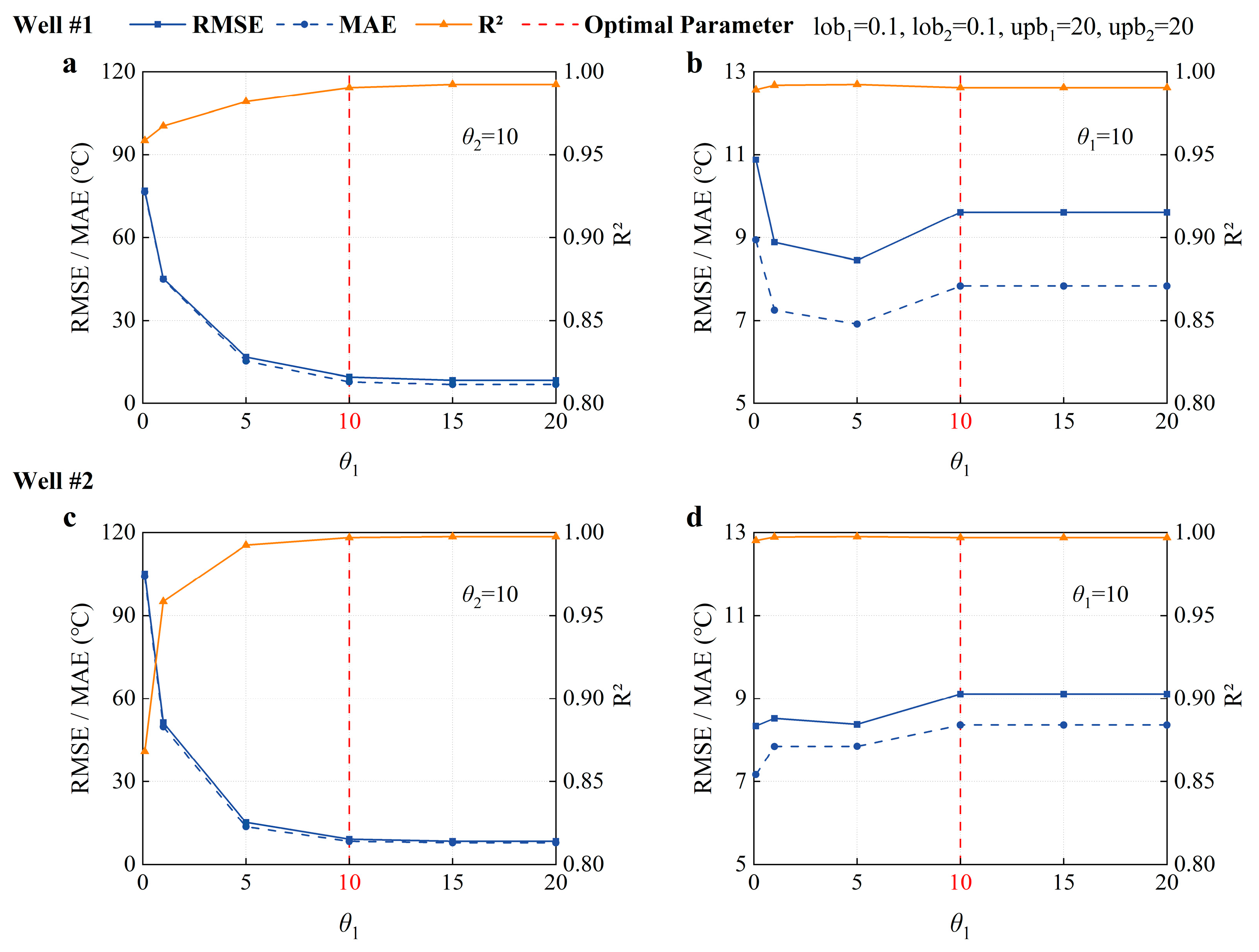
• Sensitivity Analysis of θ

The model includes two correlation length parameters, θ₁ and θ₂, which correspond to the dual-dimensional spatial structure for SFT prediction on planar surfaces. Each parameter was tested at six representative values: 0.1, 1, 5, 10, 15, and 20. As shown in Figure 7, the model exhibited notable sensitivity to the selection of θ.

For θ₁, smaller values (e.g., θ₁ = 0.1) resulted in poor generalization performance, likely due to overfitting to local noise and short-range variability. As θ₁ increased, the model’s accuracy improved, achieving a minimum RMSE and maximum R² at θ₁ = 10. Beyond this threshold, performance gradually declined, indicating that oversmoothing may obscure meaningful spatial variation. Thus, θ₁ = 10 was identified as the optimal value, offering a balance between local responsiveness and overall trend fidelity.

In contrast, θ₂ demonstrated a different pattern. As θ₂ increased, RMSE and MAE remained relatively stable until θ₂ reached 10, beyond which both metrics exhibited minimal fluctuation. The R² values showed no significant variation across the tested range, indicating a lower sensitivity of the model to changes in θ₂. Accordingly, θ₂ = 10 was also selected as the optimal value.

2.

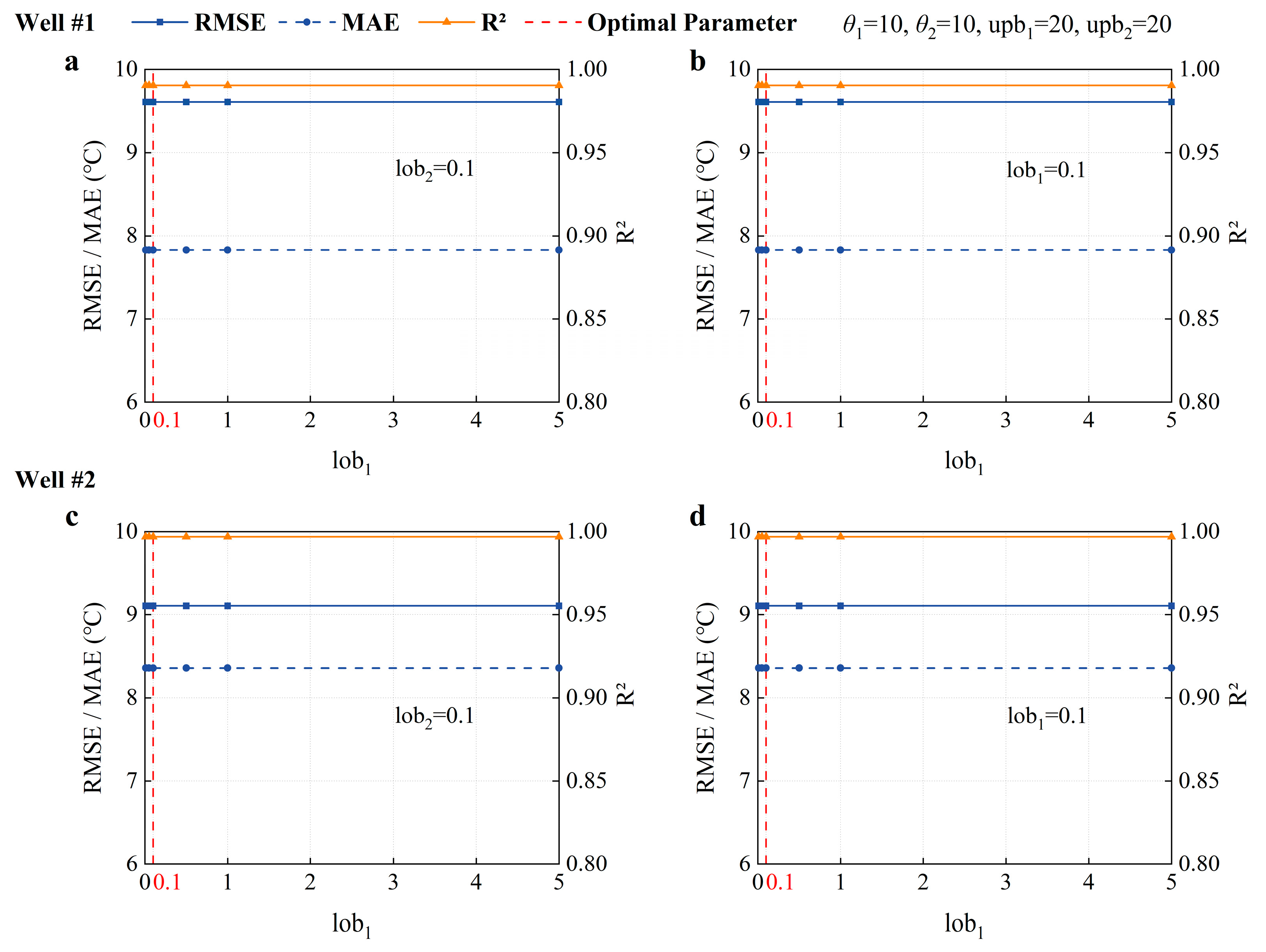
Sensitivity Analysis of lob

The lower bound (lob) defines the minimum allowable value of θ during the model’s internal optimization process. lob₁ and lob₂ represent the lower bounds for the correlation lengths θ₁ and θ₂, respectively. For each parameter, six values were evaluated: 0.01, 0.05, 0.1, 0.5, 1, and 5. As shown in Figure 8, the model’s predictive performance was largely insensitive to variations in lob₁ and lob₂. Across all tested configurations, the RMSE, MAE, and R² values remained relatively stable, indicating that changes in the lower bounds did not exert a meaningful influence on prediction accuracy. Analysis of the R² metric confirmed that the model consistently maintained high levels of fit, regardless of the lob settings. Given the lack of significant sensitivity, both lob₁ and lob₂ were assigned a value of 0.1 for subsequent model implementation. This choice aligns with common practices and serves as an empirically validated default setting for lower-bound parameters in similar geostatistical modeling applications.

3.

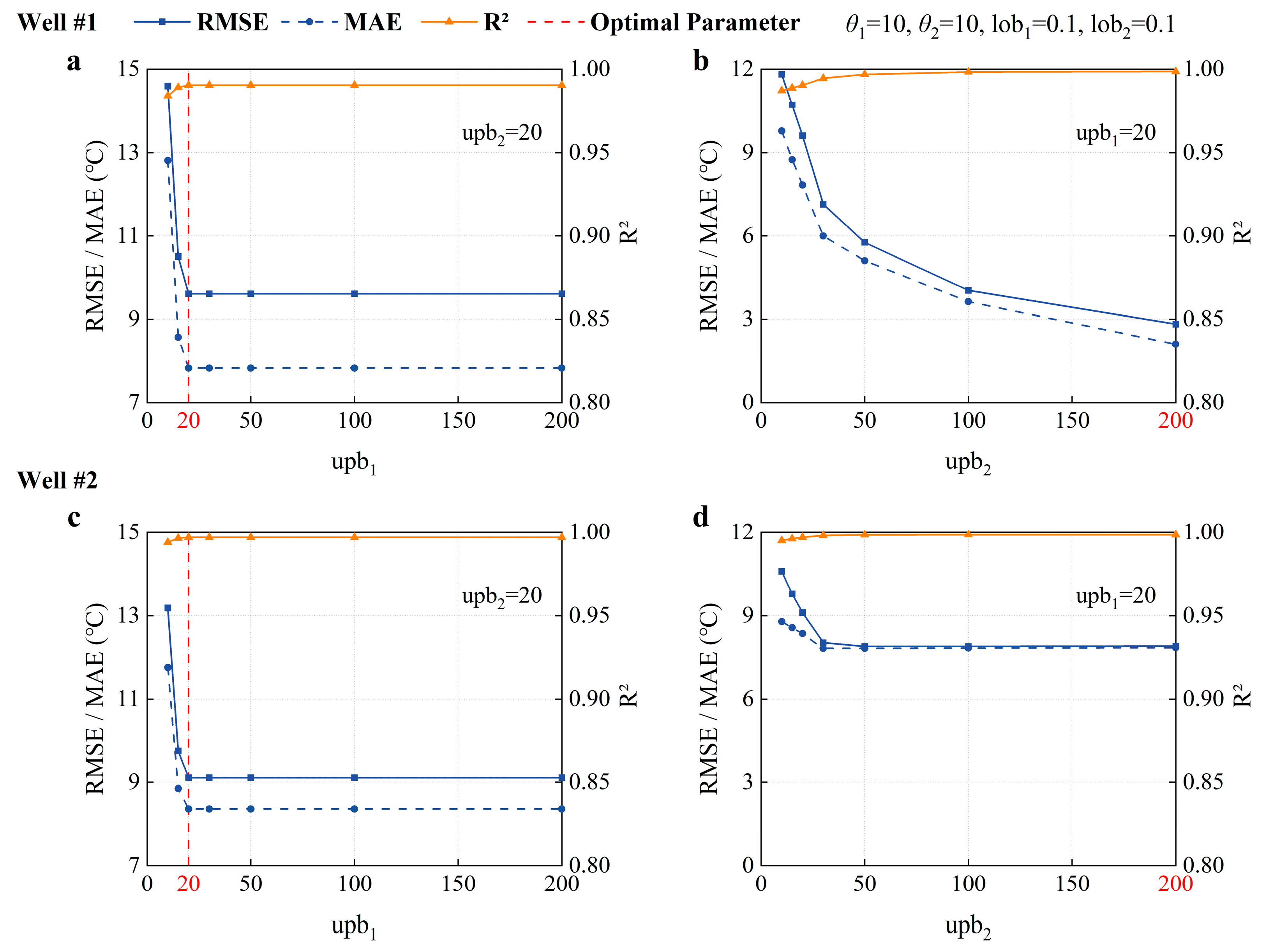
Sensitivity Analysis of upb

The upper bound (upb) defines the maximum allowable search limit for the correlation length parameter θ during the model’s internal optimization. upb₁ and upb₂ represent the upper bounds of θ₁ and θ₂, respectively. For each parameter, seven values were examined: 10, 15, 20, 30, 50, 100, and 200. As shown in Figure 9, the model exhibited clear sensitivity to upb₁. Prediction accuracy improved rapidly with increasing upb₁ values and reached optimal performance at upb₁ = 20, beyond which no significant improvement was observed. This saturation behavior supports the selection of 20 as the optimal upper bound for θ₁. For upb₂, a similar upward trend in accuracy was observed, although the improvement was more gradual across the tested range. Notably, certain well cases demonstrated continued enhancement in prediction precision as upb₂ increased. Based on empirical observations, the optimal value for upb₂ was determined to be 200, marking the point at which performance gains plateaued. Accordingly, the final parameter configuration adopted in this study was upb = [20, 200], providing a robust balance between interpolation accuracy and computational efficiency.

Based on the results of the sensitivity analyses shown in Figure 7, Figure 8 and Figure 9, the optimal set of hyperparameters for the Kriging model parameters was determined to be: θ = [10, 10], lob = [0.1, 0.1], and upb = [20, 200]. This configuration provided the best balance between interpolation accuracy and model robustness, resulting in the lowest values of RMSE and MAE while maintaining a high R². Although these parameters may not yield the optimal model accuracy for SFT prediction in other regions, they can still maintain a high level of predictive accuracy. When applying this model in other regions, it is better to conduct hyperparameter sensitivity analysis again to achieve higher accuracy.

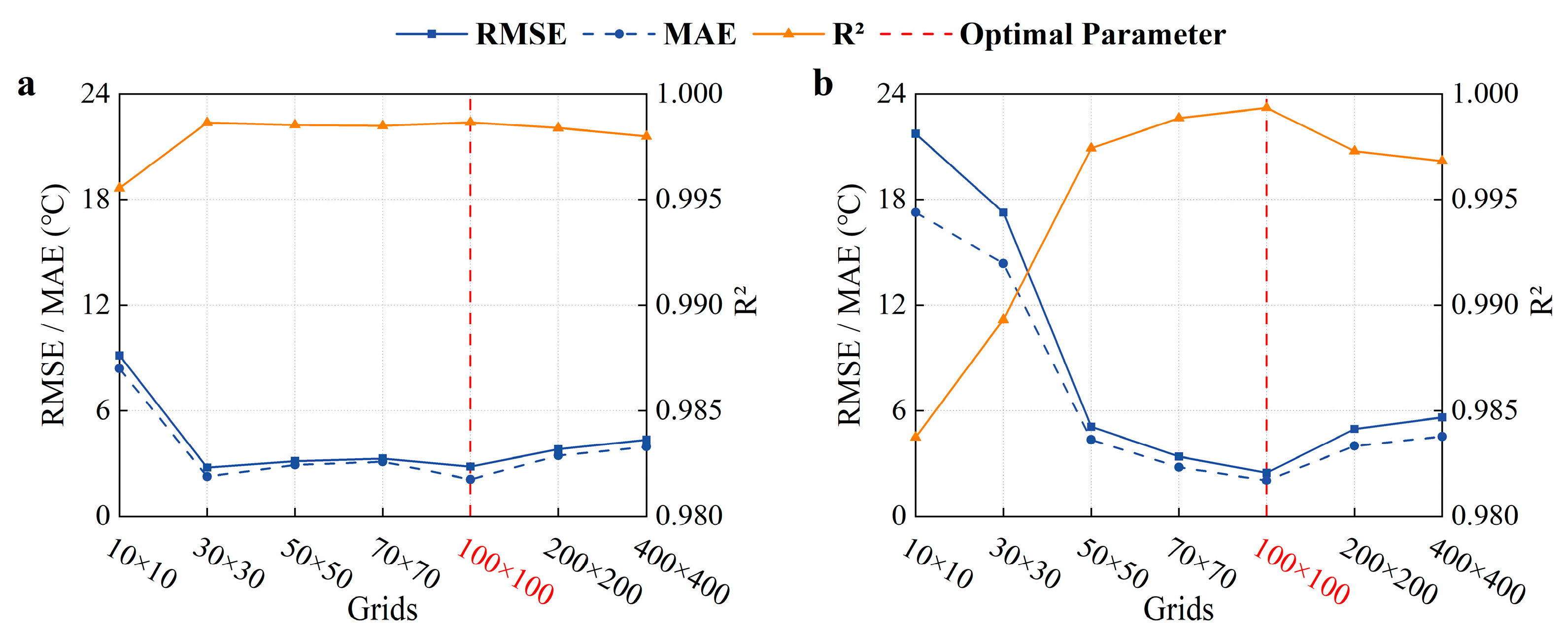
3.2. Grid Independence Analysis

In Kriging-based spatial interpolation, the selection of grid resolution plays a critical role in balancing prediction accuracy and computational efficiency. To ensure that the final temperature prediction results are not significantly affected by the discretization level, a grid independence analysis was conducted. The goal of this analysis was to identify a grid resolution that provides sufficient accuracy without incurring excessive computational cost.

Seven grid configurations were evaluated, ranging from coarse to fine resolutions: 10 × 10, 30 × 30, 50 × 50, 70 × 70, 100 × 100, 200 × 200, and 400 × 400. For each configuration, the SFT was interpolated at a fixed depth slice, and model performance was assessed based on RMSE and total computation time.

As shown in Figure 10, the variation in prediction accuracy with respect to grid resolution exhibited a similar trend across both wells. Initially, increasing the number of grid cells led to a rapid improvement in accuracy. However, beyond a certain point, further refinement resulted in diminishing returns and even a slight degradation in performance. This was attributed to oversmoothing and overfitting effects introduced by excessive grid refinement. Conversely, overly coarse grids caused excessive spatial averaging, masking local temperature variations, and reducing model fidelity.

Computation time (t_cal) serves as a crucial metric for identifying the optimal grid configuration. As illustrated in Figure 11, the computational time increases significantly with the number of grid cells. However, beyond a grid size of 100 × 100, the extended computation time does not yield improved accuracy. Considering both prediction accuracy and computational cost, the 100 × 100 grid resolution was identified as the optimal configuration. This resolution provides a balance between adequate spatial detail and computational efficiency, and was thus adopted as the standard grid setup for all subsequent Kriging-based SFT predictions in this study.

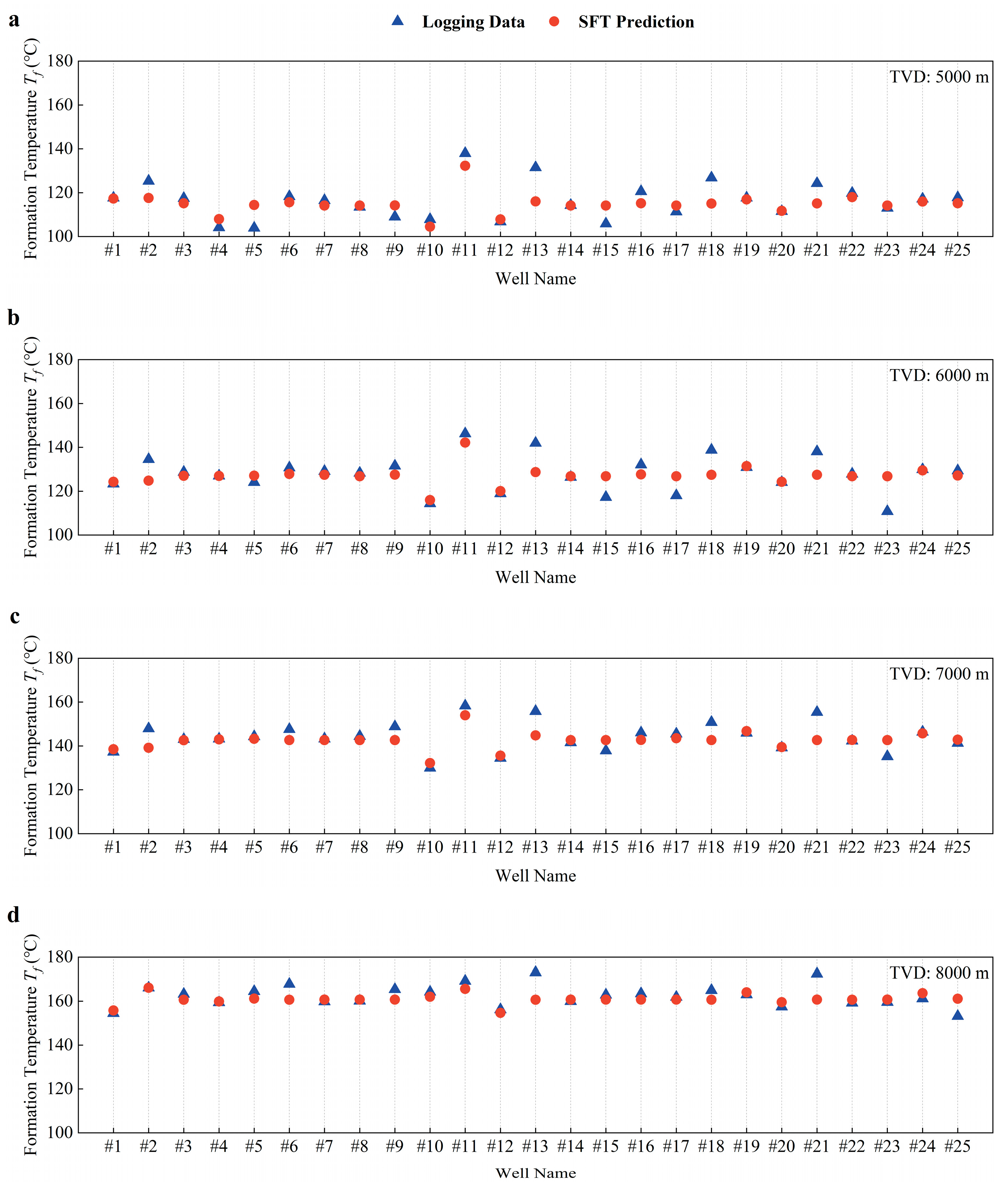
3.3. Depth-Dependent Validation Against Measured Formation Temperature Data

To further validate the reliability and generalization capability of the Kriging interpolation model across different locations, SFT profiles from four representative wells were compared against the corresponding Kriging-predicted results. These wells were deliberately selected to span multiple fault zones and diverse spatial locations within the study area, thereby ensuring a comprehensive assessment across different structural conditions.

As shown in Figure 12, the Kriging-predicted SFT profiles closely match the overall trend of the measured temperature data throughout the entire depth range. In these two wells, the predicted temperature exhibits a consistent increase with depth, and the relative prediction error is basically below 5%. Minor deviations observed at shallow and deep sections of certain wells are attributed to either limited nearby data density or localized thermal anomalies not fully captured by the regional interpolation model. Nevertheless, the close alignment between measured and predicted values demonstrates the robustness and spatial adaptability of the proposed Kriging framework.

The consistent agreement between predicted and measured temperature profiles across multiple wells underscores the robustness of the Kriging model in high-temperature, structurally complex formations. The smoothness of the predicted curves further reflects the model’s ability to filter local noise while preserving the fundamental thermal trends effectively. This multi-well validation strongly supports the conclusion that, when appropriately calibrated, the Kriging-based framework can deliver accurate and spatially reliable SFT predictions across a broad range of depths and structural conditions.

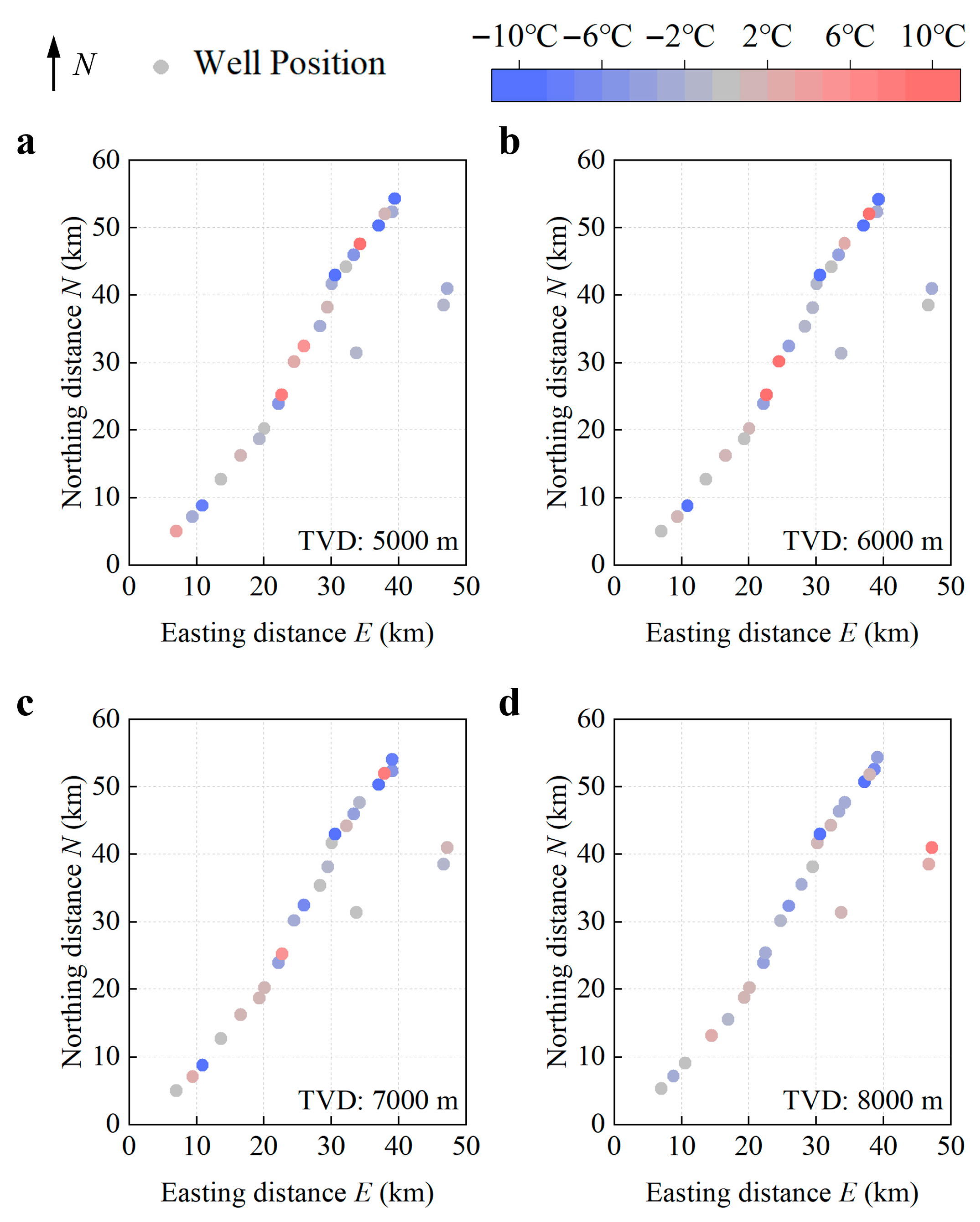
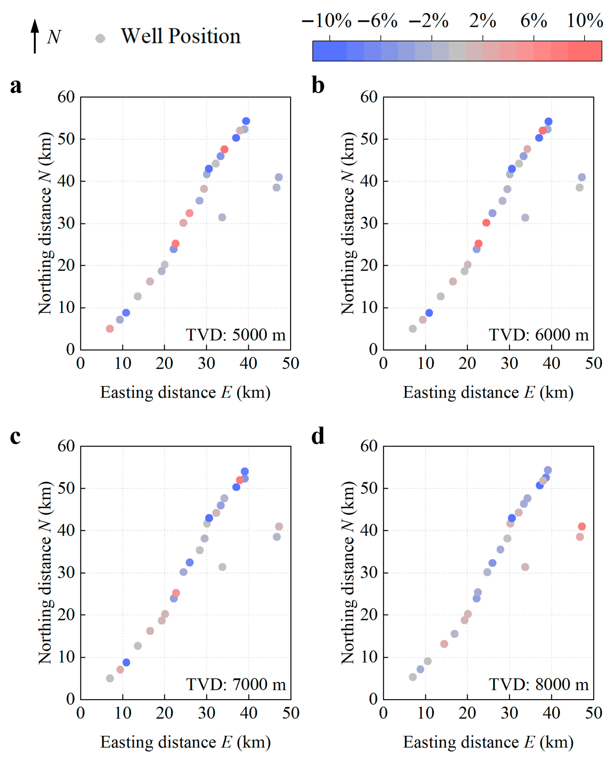
3.4. Spatial Analysis of Interpolation Errors in SFT Prediction

A detailed interpolation error analysis across selected depth planes was conducted to further assess the spatial accuracy of the Kriging-based SFT prediction model. Measured logging temperatures at four different depth planes (5000 m, 6000 m, 7000 m, and 8000 m) were compared against the Kriging-interpolated values. As shown in Figure 13, most interpolation errors for fault zone #2 remain within ±5 °C, with only a few isolated wells exhibiting slightly higher deviations. Figure 14 and Figure 15 present the spatial distribution of these errors, demonstrating an overall uniformity and the absence of localized clustering. Moreover, no evident systematic bias (i.e., consistent overestimation or underestimation) was observed across the field. These results collectively confirm that the proposed interpolation framework delivers highly accurate and spatially consistent temperature predictions, even at complex stratigraphic levels.

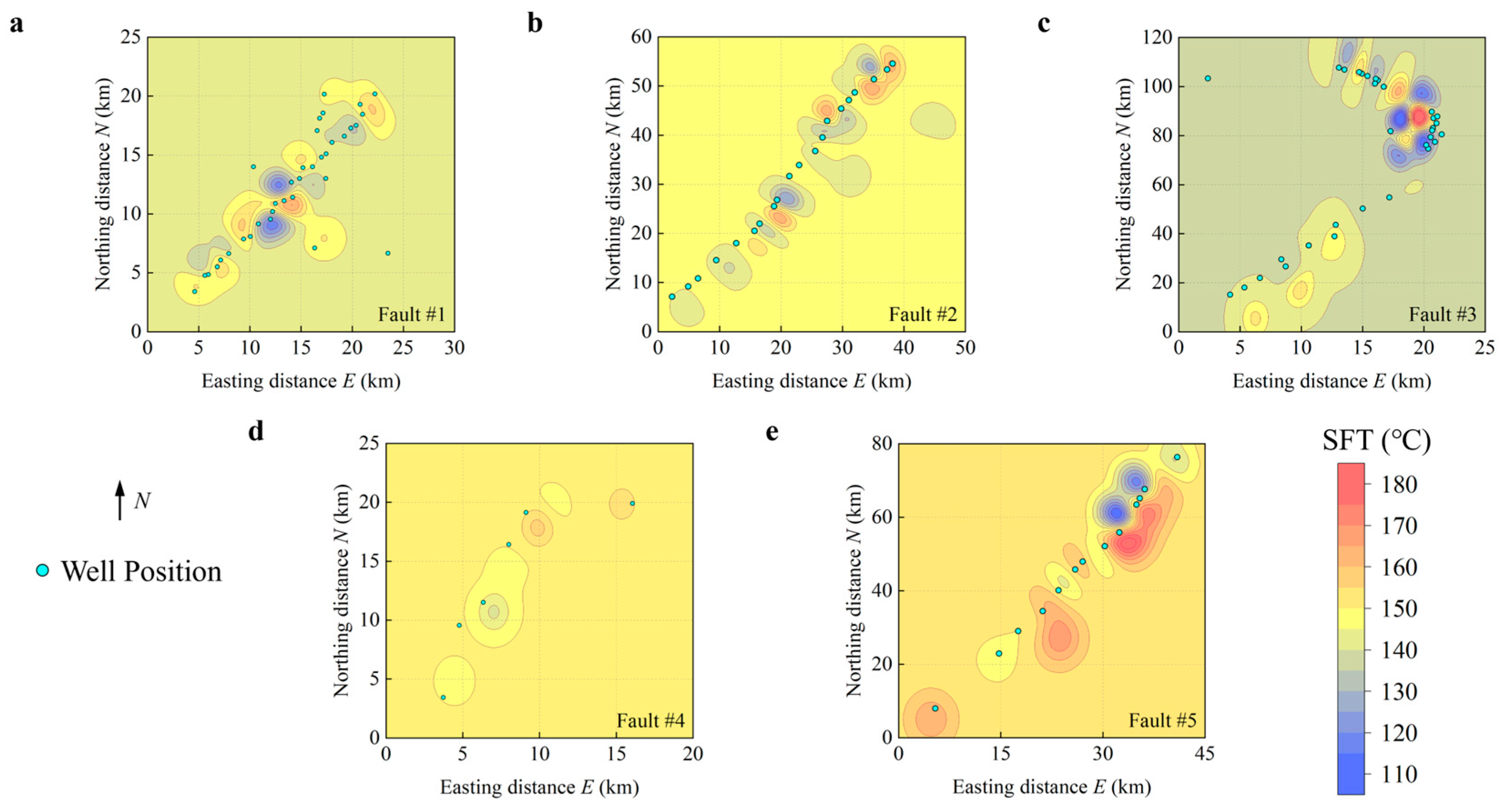
3.5. SFT Prediction of Each Fault

Based on the SFT prediction model and the spatial distribution of well locations within each fault block, SFT contour maps were generated at a depth of 7000 m for each fault zone, as shown in Figure 16. These maps depict the spatial variation in formation temperature within each zone, revealing that SFTs generally range from 130 °C to 170 °C. The color contours represent the average SFT values across the vicinity of each fault zone, providing a visual summary of localized thermal conditions.

The results indicate that, across the five fault zones, there is no pronounced trend in SFT variation along the north–south direction. However, a clear increasing gradient is observed from west to east, suggesting regional geothermal anomalies or structural influences. The predicted SFT distribution patterns are in good agreement with the temperature profiles obtained from well logging data, thereby validating the reliability of the Kriging-based interpolation framework in capturing the spatial heterogeneity of formation temperature in ultra-deep reservoirs.

4. Conclusions

(1)

This study presents a novel pseudo-3D Kriging interpolation framework incorporating actual wellbore trajectories for pre-drilling SFT prediction in ultra-deep wells. This approach overcomes the limitations of existing methods by leveraging spatial autocorrelation, establishing an efficient and accurate prediction framework.

(2)

Rigorous sensitivity analysis determined the optimal hyperparameters: correlation length θ = [10, 10], lower bound lob = [0.1, 0.1], and upper bound upb = [20, 200]. This configuration minimized prediction errors (RMSE, MAE) while maximizing R². Grid independence analysis confirmed that a 100 × 100 resolution achieves the optimal balance between accuracy and computational feasibility.

(3)

Validation using over 5.1 million SFT data points from 113 wells in the Shunbei Oilfield demonstrated exceptional model reliability. The predicted temperature profiles closely matched measured logging data across all depths, with relative errors (RE) consistently below 5%. Spatial error analysis revealed interpolation deviations predominantly within 5 °C, uniformly distributed without systemic bias. The model successfully captured the observed trend of temperature increasing west-to-east across the fault zones.

(4)

This method provides groundbreaking engineering value by enabling pseudo-3D pre-drilling SFT prediction. Unlike methods yielding averaged gradients, it delivers detailed temperature distributions for undrilled sections, enabling proactive mitigation of drilling risks caused by temperatures exceeding 150 °C. The optimized Kriging framework combines robustness with computational manageability, proving particularly effective for complex well architectures in ultra-deep reservoirs.

References

1. Lei, Q.; Xu, Y.; Yang, Z.; Cai, B.; Wang, X.; Zhou, L.; Liu, H.; Xu, M.; Wang, L.; Li, S. Progress and development directions of stimulation techniques for ultra-deep oil and gas reservoirs. Pet. Explor. Dev. 2021, 48, 221–231. [Google Scholar] [CrossRef]
2. Guo, X.; Hu, D.; Li, Y.; Duan, J.; Zhang, X.; Fan, X.; Duan, H.; Li, W. Theoretical Progress and Key Technologies of Onshore Ultra-Deep Oil/Gas Exploration. Engineering 2019, 5, 458–470. [Google Scholar] [CrossRef]
3. Khaled, M.S.; Chen, D.; Ashok, P.; van Oort, E. Drilling heat maps for active temperature management in geothermal wells. SPE J. 2023, 28, 1577–1593. [Google Scholar] [CrossRef]
4. Khaled, M.S.; Wang, N.; Ashok, P.; van Oort, E. Downhole heat management for drilling shallow and ultra-deep high enthalpy geothermal wells. Geothermics 2023, 107, 102604. [Google Scholar] [CrossRef]
5. Yao, X.; Song, X.; Zhou, M.; Xu, Z.; Duan, S.; Li, Z.; Li, H. A modified heat transfer model for predicting wellbore temperature in ultra-deep drilling with insulated drill pipe. Energy 2025, 331, 136981. [Google Scholar] [CrossRef]
6. Lv, Y.-G.; Chu, W.-X.; Wang, Q.-W. Thermal management systems for electronics using in deep downhole environment: A review. Int. Commun. Heat Mass Transf. 2022, 139, 106450. [Google Scholar] [CrossRef]
7. Wang, J.; Nitschke, F.; Gholami Korzani, M.; Kohl, T. Temperature log simulations in high-enthalpy boreholes. Geotherm. Energy 2019, 7, 32. [Google Scholar] [CrossRef]
8. Bassam, A.; Santoyo, E.; Andaverde, J.; Hernández, J.A.; Espinoza-Ojeda, O.M. Estimation of static formation temperatures in geothermal wells by using an artificial neural network approach. Comput. Geosci. 2010, 36, 1191–1199. [Google Scholar] [CrossRef]
9. Dowdle, W.L.; Cobb, W.M. Static Formation Temperature From Well Logs–An Empirical Method. J. Pet. Technol. 1975, 27, 1326–1330. [Google Scholar] [CrossRef]
10. Brennand, A.W. A new method for the analysis of static formation temperature test. In Proceedings of the the 6th New Zealand Geothermal Workshop, Auckland, New Zealand, 7 November 1984. [Google Scholar]
11. Kutasov, I.M.; Eppelbaum, L.V. A new method for determining the formation temperature from bottom-hole temperature logs. J. Pet. Gas Eng. 2010, 1, 1–8. [Google Scholar] [CrossRef]
12. Leblanc, Y.; Pascoe, L.J.; Jones, F.W. The temperature stabilization of a borehole. Geophysics 1981, 46, 1301–1303. [Google Scholar] [CrossRef]
13. Manetti, G. Attainment of temperature equilibrium in holes during drilling. Geothermics 1973, 2, 94–100. [Google Scholar] [CrossRef]
14. Ascencio, F.; García, A.; Rivera, J.; Arellano, V. Estimation of undisturbed formation temperatures under spherical-radial heat flow conditions. Geothermics 1994, 23, 317–326. [Google Scholar] [CrossRef]
15. Hasan, A.R.; Kabir, C.S. Static Reservoir Temperature Determination from Transient Data after Mud Circulation. SPE Drill. Complet. 1994, 9, 17–24. [Google Scholar] [CrossRef]
16. Al-Fakih, A.; Kaka, S. Application of Artificial Intelligence in Static Formation Temperature Estimation. Arab. J. Sci. Eng. 2023, 48, 16791–16804. [Google Scholar] [CrossRef]
17. Espinosa-Paredes, G.; Morales-Díaz, A.; Olea-González, U.; Ambriz-Garcia, J.J. Application of a proportional-integral control for the estimation of static formation temperatures in oil wells. Mar. Pet. Geol. 2009, 26, 259–268. [Google Scholar] [CrossRef]
18. Yang, M.; Tang, D.; Chen, Y.; Li, G.; Zhang, X.; Meng, Y. Determining initial formation temperature considering radial temperature gradient and axial thermal conduction of the wellbore fluid. Appl. Therm. Eng. 2019, 147, 876–885. [Google Scholar] [CrossRef]
19. Ibrahim, B.; Konduah, J.O.; Ahenkorah, I. Predicting reservoir temperature of geothermal systems in Western Anatolia, Turkey: A focus on predictive performance and explainability of machine learning models. Geothermics 2023, 112, 102727. [Google Scholar] [CrossRef]
20. Varol Altay, E.; Gurgenc, E.; Altay, O.; Dikici, A. Hybrid artificial neural network based on a metaheuristic optimization algorithm for the prediction of reservoir temperature using hydrogeochemical data of different geothermal areas in Anatolia (Turkey). Geothermics 2022, 104, 102476. [Google Scholar] [CrossRef]
21. Tut Haklidir, F.S.; Haklidir, M. Prediction of Reservoir Temperatures Using Hydrogeochemical Data, Western Anatolia Geothermal Systems (Turkey): A machine learning approach. Nat. Resour. Res. 2020, 29, 2333–2346. [Google Scholar] [CrossRef]
22. Haklidir, F.T. Hydrogeochemical evaluation of thermal, mineral and cold waters between Bursa city and Mount Uludağ in the South Marmara region of Turkey. Geothermics 2013, 48, 132–145. [Google Scholar] [CrossRef]
23. Yang, F.; Zhu, R.; Zhou, X.; Zhan, T.; Wang, X.; Dong, J.; Liu, L.; Ma, Y.; Su, Y. Artificial neural network based prediction of reservoir temperature: A case study of Lindian geothermal field, Songliao Basin, NE China. Geothermics 2022, 106, 102547. [Google Scholar] [CrossRef]
24. Pérez-Zárate, D.; Santoyo, E.; Acevedo-Anicasio, A.; Díaz-González, L.; García-López, C. Evaluation of artificial neural networks for the prediction of deep reservoir temperatures using the gas-phase composition of geothermal fluids. Comput. Geosci. 2019, 129, 49–68. [Google Scholar] [CrossRef]
25. Shahdi, A.; Lee, S.; Karpatne, A.; Nojabaei, B. Exploratory analysis of machine learning methods in predicting subsurface temperature and geothermal gradient of Northeastern United States. Geotherm. Energy 2021, 9, 18. [Google Scholar] [CrossRef]
26. Okoroafor, E.R.; Smith, C.M.; Ochie, K.I.; Nwosu, C.J.; Gudmundsdottir, H.; Aljubran, M. Machine learning in subsurface geothermal energy: Two decades in review. Geothermics 2022, 102, 102401. [Google Scholar] [CrossRef]
27. Falah, A.N.; Andriyana, Y.; Ruchjana, B.N.; Hermawan, E.; Harjana, T.; Maryadi, E.; Risyanto; Satyawardhana, H.; Sipayung, S.B. An Expanded Spatial Durbin Model with Ordinary Kriging of Unobserved Big Climate Data. Mathematics 2024, 12, 2447. [Google Scholar] [CrossRef]
28. Shanmugam, N.S.; Chen, S.-E.; Tang, W.; Chavan, V.S.; Diemer, J.; Allan, C.; Shukla, T.; Chen, T.; Slocum, Z.; Janardhanam, R. Spatial Interpolation of Bridge Scour Point Cloud Data Using Ordinary Kriging Method. J. Perform. Constr. Facil. 2025, 39, 06024002. [Google Scholar] [CrossRef]
29. Gu, Y.; Rühaak, W.; Bär, K.; Sass, I. Using seismic data to estimate the spatial distribution of rock thermal conductivity at reservoir scale. Geothermics 2017, 66, 61–72. [Google Scholar] [CrossRef]
30. Jeong, K.; Hong, T.; Chae, M.; Kim, J.; Lee, M.; Koo, C.; Ji, C. Development of the hybrid model for estimating the undisturbed ground temperature using the finite element method and geostatistical technique. Energy Build. 2017, 152, 162–174. [Google Scholar] [CrossRef]
31. Che, D.; Jia, Q. Three-Dimensional Geological Modeling of Coal Seams Using Weighted Kriging Method and Multi-Source Data. IEEE Access 2019, 7, 118037–118045. [Google Scholar] [CrossRef]
32. Su, F.-Q.; Yang, J.-N.; He, X.-L.; Dai, M.-J.; Hamanaka, A.; He, Y.Y.; Li, W.; Li, J.-Y. Influences of removable gas injection methods on the temperature field and gas composition of the underground coal gasification process. Fuel 2024, 363, 130953. [Google Scholar] [CrossRef]
33. Agemar, T.; Schellschmidt, R.; Schulz, R. Subsurface temperature distribution in Germany. Geothermics 2012, 44, 65–77. [Google Scholar] [CrossRef]
34. Sepúlveda, F.; Rosenberg, M.D.; Rowland, J.V.; Simmons, S.F. Kriging predictions of drill-hole stratigraphy and temperature data from the Wairakei geothermal field, New Zealand: Implications for conceptual modeling. Geothermics 2012, 42, 13–31. [Google Scholar] [CrossRef]
Figure 1. Process of SFT-derived wellbore temperature calculations.
Processes 13 02303 g001
Figure 2. Distribution of Faults in Shunbei Oilfield.
Processes 13 02303 g002
Figure 3. Distribution of SFT ranges across each fault zone.
Processes 13 02303 g003
Figure 4. Full-borehole logging temperature data of two wells: (a) well from fault #4; (b) well from fault #5.
Processes 13 02303 g004
Figure 5. Wellbore temperature profiles from multiple drilling phases.
Processes 13 02303 g005
Figure 6. Filtering process for raw well-logging temperature data with fluctuations.
Processes 13 02303 g006
Figure 7. Sensitivity analysis of θ on model performance: (a) θ1 of well #1; (b) θ2 of well #1; (c) θ1 of well #2; and (d) θ2 of well #2.
Processes 13 02303 g007
Figure 8. Effect of lower bound (lob) on Kriging model accuracy: (a) lob1 of well #1; (b) lob2 of well #1; (c) lob1 of well #2; and (d) lob2 of well #2.
Processes 13 02303 g008
Figure 9. Effect of upper bound (upb) on Kriging model accuracy: (a) upb1 of well #1; (b) upb2 of well #1; (c) upb1 of well #2; and (d) upb2 of well #2.
Processes 13 02303 g009
Figure 10. Grid independence analysis: effect of grid resolution on RMSE, MAE, and R2. (a) grid independence analysis of well #1; (b) grid independence analysis of well #2.
Processes 13 02303 g010
Figure 11. Computation time of the model versus number of grid cells.
Processes 13 02303 g011
Figure 12. Comparison of measured and Kriging-predicted SFT profiles for six representative wells: (a) Well #1; (b) Well #3; (c) Well #4; (d) Well #7; (e) Well #8; (f) Well #19.
Processes 13 02303 g012
Figure 13. Comparison between logging temperature and SFT prediction of fault #2: (a) TVD = 5000 m; (b) TVD = 6000 m; (c) TVD = 7000 m; and (d) TVD = 8000 m.
Processes 13 02303 g013
Figure 14. Spatial distribution of absolute errors during interpolation of fault #2. (a) TVD = 5000 m; (b) TVD = 6000 m; (c) TVD = 7000 m; and (d) TVD = 8000 m.
Processes 13 02303 g014
Figure 15. Spatial distribution of relative errors during interpolation of fault #2. (a) TVD = 5000 m; (b) TVD = 6000 m; (c) TVD = 7000 m; and (d) TVD = 8000 m.
Processes 13 02303 g015
Figure 16. SFT prediction for each fault at 7000 m: (a) SFT prediction for fault #1; (b) SFT prediction for fault #2; (c) SFT prediction for fault #3; (d) SFT prediction for fault #4; and (e) SFT prediction for fault #5.
Processes 13 02303 g016