Abstract
Power flow analysis of low-voltage network (LVN) is one of the most crucial methods for achieving refined management of such networks. To accurately calculate the three-phase (TP) probabilistic power flow (PPF) distribution in LVN, this paper first draws on the injection-type Newton method; by leveraging TP power measurements relative to the neutral point obtained from smart meters, the injected power is expressed in terms of injected current equations, thereby establishing TP power flow models for various components within the low-voltage distribution transformer area grid. Subsequently, addressing the stochastic fluctuation models of load power and photovoltaic output, this paper employs conventional numerical methods and an improved Latin hypercube sampling technique. Utilizing linearized power flow equations and based on the improved semi-invariant method (SIM) and Gram–Charlier (GC) series fitting, a calculation method for three-phase PPF in low-voltage distribution transformer area grids using the improved semi-invariant is proposed. Finally, simulations of the proposed three-phase PPF method are conducted using the IEEE-13 node distribution system. The simulation results demonstrate that the proposed method can effectively perform three-phase PPF calculations for the distribution transformer area grid and accurately obtain probabilistic distribution information of the TP power flow within the grid.
1. Introduction
With the ever-growing integration of distributed photovoltaic (PV) and wind energy systems into the power grid, the uncertain nature of their power outputs has introduced substantial variability to the grid’s power flow dynamics [1,2,3,4]. Traditional deterministic approaches to power flow calculation, including the forward–backward sweep method and the cyclic iterative Newton–Raphson method, fall short in comprehensively capturing these uncertainties and their impacts on the system. Consequently, these methods are ill-suited for scenarios involving distributed energy resources [5,6,7,8]. In contrast, the analytical probabilistic power flow (PPF) calculation method stands out for its ability to integrate the uncertainties stemming from distributed energy resources and load fluctuations directly into the power flow equations. This integration is achieved without imposing significant computational demands, all the while maintaining a satisfactory level of accuracy. As a result, the PPF calculation method has garnered widespread acceptance and popularity among researchers [9,10,11].
In prior studies, Monte Carlo (MC) simulation analysis techniques have emerged as powerful tools for characterizing uncertain variables. These techniques facilitate the examination of uncertainties and unobservable phenomena within distribution systems, as well as the evaluation of uncertainties pertaining to network power flow [12,13,14,15]. For instance, reference [16] employs MC simulation to capture the fluctuations in load and PV output across the network. By delineating scenarios involving line insulation degradation and modeling impedance variations, it constructs a framework for probabilistic power flow (PPF) calculation. On the other hand, reference [17] presents a PPF calculation method grounded in cumulants and the GC series. This method takes into account uncertainties such as wind turbine output variability, load fluctuations, and line faults. By computing the cumulants of injected power at each node using node voltage and branch power sensitivity matrices, it proposes a PPF calculation approach based on cumulants and the GC series expansion.
The network architecture of low-voltage distribution area grids is notably intricate, characterized by a substantial number of end-user loads and a significant degree of TP imbalance. As PV systems become increasingly integrated at the end-user level within these areas, the uncertainty associated with power flow in low-voltage distribution grids is escalating [18,19,20,21,22,23]. To align with the demands of smart distribution networks and facilitate refined management of distribution areas, it is crucial to consider the inherent uncertainties within these grids. In particular, performing three-phase PPF calculations for low-voltage distribution area grids is vital for accurately acquiring probabilistic distribution data regarding TP power flow across the network. This, consequently, offers more thorough and dependable reference information and a solid foundation for decision-making in the refined management of the LVN [24,25].
To tackle this issue, this paper initially leverages the injection-type Newton method and makes use of the three-phase power measurements with respect to the neutral point, which are collected from smart meters. By formulating the injected power as injected current equations, we construct a TP power flow model for every component within the low-voltage distribution area grid. Next, taking into account the stochastic fluctuation models of load power and PV output, we adopt conventional numerical methods along with an enhanced Latin hypercube sampling technique to manage these uncertainties. Utilizing linearized power flow equations, we put forward a three-phase PPF calculation method tailored for low-voltage distribution area grids. This method is based on an improved semi-invariant approach and Gram–Charlier series fitting. Finally, the effectiveness of the proposed three-phase PPF method is verified through simulations conducted on the IEEE-13 node distribution system.
2. TP Power Flow Models for Components in LVN
2.1. The Mathematical Model of LVN Line
In LVN, the three-phase four-wire line model is illustrated in Figure 1 [26]. In LVN, the three-phase four-wire line model is depicted in Figure 1. In the figure, k() represents the node number of the line; (,) denotes the voltage of phase at node k; indicates the current of phase at node k; represents the currents of phase at nodes i and j; () signifies the branch impedance ( being the self-impedance and being the mutual impedance).
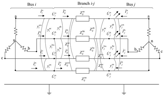
Figure 1.
Low-voltage line equivalent model.
The branch impedance matrix is given as follows:
where and (, ,) represent the self-impedance and mutual impedances between nodes i and j, respectively.
2.2. The Mathematical Model of LVN Load
For the loads in low-voltage distribution area grids, where the given quantities are the powers measured by smart meters relative to the neutral point, the expression for converting these into node injection currents based on the injection-type Newton’s method is as follows:
where () represents the load power of phase d; denotes the voltage of phase d; indicates the current of phase d; is the neutral current; and is the neutral voltage.
For a single-phase load, the injection current calculation formula (taking phase a as an example) is:
where represents the load power of phase a; denotes the voltage of phase a; indicates the current of phase a.
2.3. The Mathematical Model of LVN Power Source
In LVN, the low-voltage side of the LVN is typically designated as the balance node, serving as the power supply node for the low-voltage distribution network. When distributed generation (DG) units are connected to the distribution area grid and modeled as PQ nodes with constant active and reactive power outputs, their representation is identical to that of loads—the key difference being that loads absorb power while DG units inject power. If the DG unit has sufficient reactive power capacity to maintain a constant voltage magnitude, it can be treated as a PV node, with its model described as follows:
3. MC Simulation for Probabilistic Power Flow Calculation
3.1. Stochastic Fluctuation Model for Load Power
Mathematical statistics indicate that the Gaussian distribution can approximately describe the stochastic characteristics of load power over a certain period. The probability density function (PDF) of the Gaussian distribution is given by:
where PL represents the load power; f denotes the PDF; σL indicates the standard deviation; PL,Mean signifies the mathematical expectation (mean) of the load power.
3.2. Stochastic Fluctuation Model for PV Output
Mathematical statistics indicate that, over a certain period, the solar irradiance affecting PV output can be modeled using the Beta distribution to describe its stochastic behavior. The PDF is given by the following equation:
where α and β represent the parameters in Beta distribution; f denotes the probability density; r indicates the solar irradiance; rmax signifies the maximum solar irradiance.
The relationship between PV active power output and solar irradiance is expressed as:
where A represents the number of PV modules; η denotes the photoelectric conversion efficiency; PDG indicates the PV active power output.
From the above two equations, we can obtain:
where PDG,max can be expressed as the maximum PV power output.
3.3. Mathematical Significance of Probabilistic Power Flow
The mathematical significance of probabilistic power flow can be characterized as follows: Given the PDF of the input vector X and the mapping relationship defined by Equation (10), the objective is to derive the PDF of the output vector Z. However, in power systems, the power flow expressions are inherently nonlinear, and in practice, only the inverse mapping g−1 (as shown in Equation (11)) can be explicitly formulated. Mathematically, the direct mapping g cannot be obtained analytically due to the following reasons:
where f and g represent the power flow equations; X is the vector of nodal injection powers; Z is the vector of unknown power flow variables to be solved.
3.4. MC Simulation Technique
The MC simulation method, a well-established statistical simulation technique, adopts the following core strategy for probabilistic computations [27,28]. When dealing with a specific set of random variables, random number generators are employed to produce samples. Leveraging pre-defined mathematical mapping relationships, a substantial number of mapped samples for unknown quantities are derived from known values. Subsequently, by performing statistical analysis on these large-scale data samples, the frequency distribution characteristics of the unknown variables can be determined. In accordance with the Law of Large Numbers, as the sample size reaches a sufficiently large magnitude, the frequency distribution will closely resemble the actual probability distribution.
As a highly adaptable sampling-based simulation approach, MC simulation is unrestricted by the field of application or the inherent intricacy of the problem at hand, which makes it well-suited for PPF analysis. Nevertheless, its high computational demands make it unfeasible for practical real-world applications. In academic research, PPF results derived from MC simulations using a large number of samples are commonly considered as the gold-standard reference results for validating the accuracy of other algorithms. Similarly, in this study, we utilize the results of MC simulation as a benchmark to confirm the efficacy of the proposed method. A schematic diagram depicting the PPF calculation process based on MC simulation is presented in Figure 2.
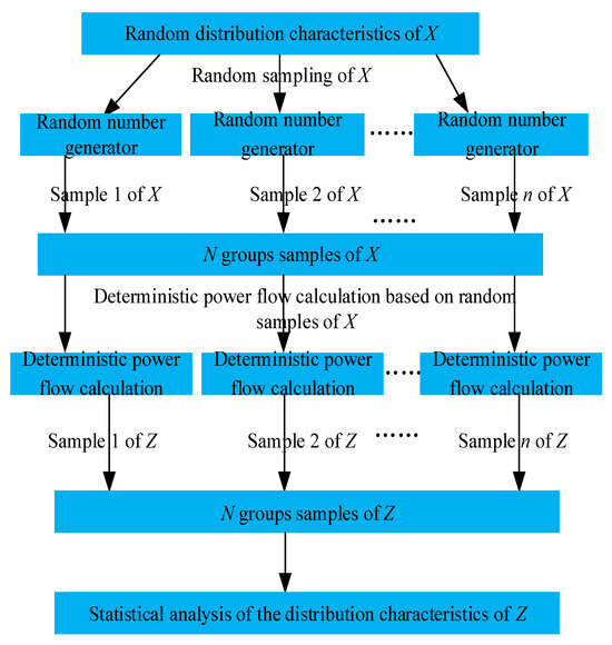
Figure 2.
PPF calculation diagram based on MC simulation method.
4. Three-Phase PPF Calculation Method for LVN Based on an Improved SIM
4.1. Linearization of Nonlinear Power Flow Equations
By performing a Taylor expansion of Equation (11) around the mean value Z0 of Z, and neglecting second-order and higher-order terms, Equation (12) is obtained:
where Z0 denotes the mean value of Z; T is the Jacobian matrix; and ΔZ represents the deviation of the power flow.
From the above Equation (12), it follows that:
where ΔX denotes the deviation of nodal injection power, and X0 is mean value of X.
Taking the inverse of Equation (12), we obtain:
It can be seen from the above the ΔZ and ΔX are linearly related. Therefore, if the components of ΔX are mutually independent, the probability distribution of ΔZ can be calculated from that of ΔX using convolution.
4.2. Improved SIM
The semi-invariant method relies on creating random sequences from random variables to calculate mathematical properties, including the expectation (the first-order raw moment), variance (the second-order central moment), and cumulants. In this research, traditional numerical techniques are utilized to produce random sequences for load power. Meanwhile, an enhanced Latin hypercube sampling (LHS) approach is adopted for generating random sequences of PV output. Here, LHS serves as an efficient and widely accepted tool for handling the randomness of PV power output and generating representative scenarios to support the aforementioned core research objectives. It is not the methodological innovation point or the primary research focus of this paper. We chose LHS due to its recognized advantages in dealing with high-dimensional input variables, improving sample space coverage efficiency, and reducing the required sample size to achieve statistical convergence. These characteristics make it particularly suitable for PV power output sampling in our study. Although MC simulation is fundamental, it converges relatively slowly. low-discrepancy sequences like Sobol sequences excel in specific integration problems, but when it comes to generating “scenario sets” for subsequent stochastic programming or probabilistic assessment, LHS offers a good balance between computational efficiency and representativeness, which is why it is widely adopted in uncertainty research within energy systems. The process for generating random sequences of PV output is outlined as follows:
- (1)
- Given that the random variable x is defined over the interval , which is equally divided into n points , the probability density at point is . Therefore, the cumulative distribution function (CDF) at can be calculated as:
- (2)
- The interval of the CDF is divided into n − 1 subintervals with spacing . On each subinterval , using the cumulative distribution y as the independent variable and the sample x as the dependent variable, a cubic interpolation is applied to establish the x-y relationship as:
- (3)
- For any given value of the cumulative distribution, must lie within a certain subinterval . By substituting into the x-y relationship, the corresponding sample can be obtained.
- (4)
- Based on the Cholesky decomposition method, the sampled samples are sorted to obtain the random sampling sequence.
After generating the random sequences for each variable, the formulas for calculating the m-th order raw moments and central moments are as follows:
where denotes the m-th order raw moment of variable ; denotes the m-th order central moment of variable ; and E denotes the expectation.
Semi-invariants can be calculated using raw moments and central moments up to the same order. The formulas for the first eight cumulants are as follows:
where table shows the m-th order cumulants (where m = 1, 2, …, 8).
Since cumulants satisfy the principle of linear superposition, based on the linear relationship between the power flow physical quantities to be determined (such as node voltage, injected power, and branch power flow) and known disturbance quantities like injected power, that is, the series of cumulants of ΔX can be used to obtain the series of cumulants of ΔZ, we can derive:
where is m-th order cumulant of ΔZ; m-th order cumulant of ΔX.
From the formula for central moments, we derive:
Thus, to determine the PDF of variables Z, the series of cumulants for Z can be calculated based on the known probability distribution of the disturbance variable X, yielding:
where Z0 represents the mean power flow solution computed using the mean values of injected power.
4.3. GC Series Fitting
Based on the series of cumulants calculated for each power flow physical quantity Z and the GC series fitting, the probability distribution function of Z can be obtained. In this paper, the first 8-th orders of cumulants are taken, and the probability density formula for Z is derived using the GC series fitting, as shown below:
where f(x) represents the PDF; x denotes the random variable; ϕ(x) represents the standard Gaussian distribution of the random variable; g denotes the normalized cumulants; H represents the Hermite polynomials.
The convergence of the GC series expansion heavily relies on the degree of approximation between the distribution to be fitted and the normal distribution. In low-voltage distribution networks incorporating strongly intermittent renewable energy sources, the probability distributions of node voltages and branch power flows often exhibit multimodality or significant skewness, necessitating high-order terms in the GC series for convergence. Additionally, when the cumulants of order four or higher for the output variables are large, the GC series may produce negative probabilities in the tail regions, violating fundamental probability axioms. The accuracy of the GC series directly depends on the precision of high-order moment estimates for input variables. For non-Gaussian renewable energy sources like wind and photovoltaic power, their output distributions inherently involve substantial estimation errors in high-order moments. Traditional GC series assume that input variables are independently and identically distributed; however, in real-world systems, spatial correlations exist among wind power, photovoltaic power, and loads. Although correlations can be addressed using techniques like the Nataf transformation or Copula functions, the transformed variables lose high-order information during GC expansion. To balance computational accuracy and numerical stability in three-phase probabilistic power flow calculations for low-voltage distribution areas, we implemented the following preprocessing steps to mitigate the aforementioned limitations:
- (1)
- Conducting a pre-normality test (using the Anderson–Darling test with a significance level of α = 0.05) on all input random variables, including wind power, photovoltaic power, and loads;
- (2)
- Setting up large-scale Monte Carlo sampling as a benchmark.
The calculation flowchart for the three-phase PPF computation method in distribution network areas based on the improved SIM is illustrated in Figure 3.
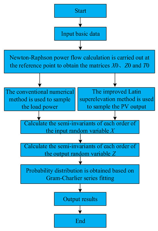
Figure 3.
Three-phase PPF calculation flow chart based on improved SIM.
5. Simulation Case Study and Analysis
5.1. Basic Data and Simulation Conditions
Based on the IEEE-13 node distribution system (rated voltage: 4.16 kV) from reference [16], simulations were conducted to validate the proposed three-phase PPF calculation method for low-voltage distribution networks using an improved cumulant-based approach. The total load in this distribution network is 3107.43 kW + j1831.83 kVar. The original load values were treated as the mean (µ), with 10% of the mean serving as the standard deviation (σ). The power base value was set to 1 MVA. PV sources with a capacity of 100 kW were installed at Node 2 and Node 11, with solar irradiance modeled using a Beta distribution (parameters: α = 0.9, β = 0.8). The topology of the IEEE-13 node distribution system is illustrated in Figure 4. In this paper, the main reasons for connecting PV sources at Node 2 and Node 11 are as follows: Node 2 is close to the main transformer node that links with the upper-level power grid, and thus can, to a certain extent, represent centralized PV systems connected at the head of the distribution area. Node 11 is located at the end of the feeder and can be used to simulate distributed PV, serving as a typical scenario for low-voltage PV integration.
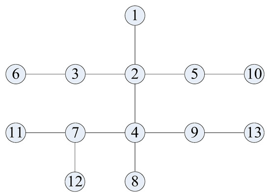
Figure 4.
IEEE-13 buses distribution system.
Although this paper adopts Gaussian distribution for loads and Beta distribution for PV systems, respectively, the proposed method itself does not rely on specific distribution types. The improved SIM can calculate cumulants for any arbitrary distribution through numerical integration, while GC series fitting only requires the input of moments at various orders and is independent of the distribution form. Moreover, this paper employs LHS to support inverse transform sampling for any cumulative distribution function. Therefore, for non-standard distribution data of loads and PV systems, this method can be directly applied without modifying the core algorithm.
To validate the effectiveness of the proposed method in this paper, we adhere to the consensus of the IEEE PES Working Group by taking traditional SIM, MC simulation, and quasi-MC simulation as direct comparison counterparts, as they share the same statistical moment-passing framework with our method, whereas polynomial chaos expansion and Gaussian process-based methods belong to different technical routes. Based on MC simulation, a sampling size of 107 times is selected to conduct MC simulation-based power flow calculations for the system. The frequency characteristics of the obtained results are then statistically analyzed and used as the standard reference results. The conventional semi-invariant method with regular numerical sampling and the three-phase PPF calculation method proposed in this paper, which is based on an improved semi-invariant approach, are employed separately to perform three-phase PPF calculations. The results obtained from these two methods are then compared with those from the 107 times MC simulation.
5.2. Simulation Results and Analysis
For the IEEE-13 node distribution system, calculations are carried out using two approaches: one involves 107 times MC simulation sampling, and the other employs the three-phase PPF calculation model established in this paper, which is based on the SIM and the improved SIM proposed in this paper. A comparison of the expected values and standard deviations of TP voltage magnitudes and injected power at nodes 4, 6, and 13 is presented in Table 1 and Table 2, respectively.

Table 1.
Comparison of voltage amplitude mean and standard deviation results.
Table 2.
Comparison of injected active power mean and standard deviation results.
Taking Node 4 as an example, as can be seen from Table 1, under the 107 times MC simulation sampling calculation, the expected values of the voltage magnitudes for phases A, B, and C at Node 4 are 0.9125, 0.9402, and 0.8751, respectively, and the standard deviations are 0.6035 × 10⁻², 0.7323 × 10⁻², and 1.0201 ×10⁻², respectively. These results are regarded as the standard reference results. Based on the SIM, the expected values of the voltage magnitudes for phases A, B, and C at Node 4 are 9.1251 × 10⁻¹, 9.4022 × 10⁻¹, and 8.7511 × 10⁻¹, respectively, and the standard deviations are 6.03505 × 10⁻³, 7.32311 × 10⁻³, and 10.2008 × 10⁻³, respectively. Using the method proposed in this paper, the expected values of the voltage magnitudes for phases A, B, and C at Node 4 are 9.12508 × 10⁻¹, 9.40213 × 10⁻¹, and 8.75104 × 10⁻¹, respectively, and the standard deviations are 6.03503 × 10⁻¹, 7.32309 × 10⁻¹, and 10.2009 × 10⁻¹, respectively.
Similarly, taking Node 4 as an example, Table 2 shows that under 107 MC simulation sampling calculations, the expected values of active power injection for Phases A, B, and C are 0.3920, 0.4170, and 0.4422, respectively, with standard deviations of 0.0387, 0.0415, and 0.0441. These results are used as the standard reference values. Based on the SIM, the expected values of active power injection for Phases A, B, and C at Node 4 are 3.9215 × 10⁻¹, 4.2722 × 10⁻¹, and 4.4231 × 10⁻¹, respectively, with standard deviations of 3.8710 × 10⁻², 4.1513 × 10⁻², and 4.4119 × 10⁻². By using the proposed method in this paper, the expected values of active power injection for Phases A, B, and C at Node 4 are 3.9211 × 10⁻¹, 4.1714 × 10⁻¹, and 4.4228 × 10⁻¹, respectively, with standard deviations of 3.8708 × 10⁻², 4.1510 × 10⁻², and 4.4108 × 10⁻².
From this, it can be seen that the errors between the voltage magnitude power flow calculation results obtained using the three-phase PPF calculation model established in this paper, which is based on the SIM and the improved SIM, and the standard reference results are all within the order of magnitude of 0.001%. The errors between the injected active power flow calculation results and the standard reference results are all within the order of magnitude of 0.01%. Both sets of results are very close to the standard reference results, and the results from the method proposed in this paper exhibit smaller errors and higher accuracy. The main reason is that during the sampling process of the proposed method, different probability characteristics of load power and PV output are taken into account. Different sampling methods are employed for sampling, and their semi-invariants are calculated accordingly. Compared with merely using conventional numerical sampling methods, this approach yields better results.
To better compare the probabilistic distribution characteristics of random variables, taking the B-phase voltage magnitude at Node 4 as an example, the PDF and cumulative distribution function (CDF) images obtained from 107 MC simulation sampling calculations, as well as those derived using the three-phase PPF computation model proposed in this paper based on the SIM and the improved SIM, are plotted in Figure 5 and Figure 6, respectively.
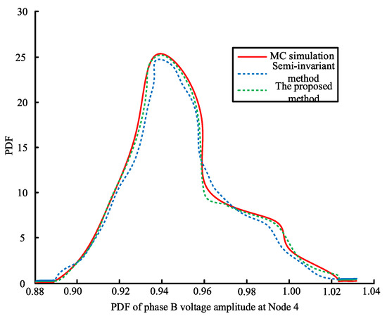
Figure 5.
PDF of phase B voltage amplitude at Node 4.
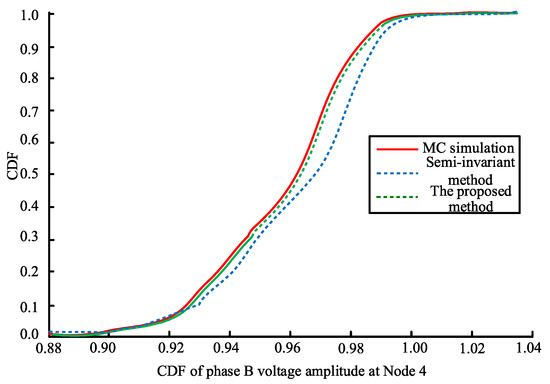
Figure 6.
CDF of phase B voltage amplitude at Node 4.
As can be seen from Figure 5 and Figure 6, the PDF images and CDF images of the B-phase voltage magnitude at Node 4 obtained using the three-phase PPF calculation model established in this paper, which is based on the SIM and the improved SIM, are essentially consistent with those obtained from the 107-time MC simulation sampling calculation. Moreover, the fitting results of the PDF and CDF images from the method proposed in this paper are even closer to the MC simulation results. This further validates that the three-phase PPF calculation method proposed in this paper offers higher accuracy, enabling effective three-phase PPF calculation for distribution network areas and accurately obtaining the probabilistic distribution information of power flow in distribution network areas.
In order to verify the calculation efficiency and convergence of the method proposed in this paper, the calculation time of the method proposed in this paper is compared with the traditional half-step variable method, MC method and quasi-MC method, and the results are shown in Table 3.
Table 3.
Comparison of computational efficiency and convergence.
As can be seen from Table 3, the improved SIM+GC series method (i.e., the proposed method) in this paper avoids repetitive power flow calculations by utilizing the linear superposition property of cumulants. The time consumption of this method mainly stems from order optimization and piecewise linearization processing. Its computational time is longer than that of the traditional SIM but significantly less than that of the MC method and the quasi-MC method. Additionally, the traditional SIM is an analytical approach with no iteration count involved, whereas the convergence of the proposed method in this paper depends on the linearization region partitioning and the selection of GC orders, and the convergence of MC simulation relies on the sample size. Therefore, the improved SIM+GC method proposed in this paper demonstrates the best performance in terms of the precision–efficiency trade-off, making it particularly suitable for probabilistic computational analysis of systems under the volatility of new energy sources.
6. Conclusions
To accurately calculate the three-phase PPF distribution in LVN, this paper proposes a three-phase PPF calculation method for LVN based on an improved SIM. This method has the following characteristics:
- (1)
- Drawing on the injection-type Newton method and based on the TP power measurements relative to the neutral point obtained from smart meters, the injected power is expressed in terms of injected current equations to establish TP power flow models for each component in the LVN.
- (2)
- For the stochastic fluctuation models of load power and PV output, conventional numerical methods and improved Latin hypercube sampling are employed, respectively. By utilizing linearized power flow equations, the PDF of the TP power flow in the LVN is calculated based on the improved SIM and GC series fitting.
- (3)
- Finally, simulation analysis of the proposed three-phase PPF method is conducted using an improved IEEE-13 node distribution system. The simulation results demonstrate that the proposed method can effectively perform three-phase PPF calculations for distribution network areas and accurately obtain the probabilistic distribution information of power flow in these areas.
In the future, we will explore the embedded application of the maximum entropy principle in the GC series, develop adaptive truncation strategies, and investigate hybrid analytical–simulation algorithms to address the deficiencies of the GC series in ultra-high-dimensional systems or extreme event analyses. In addition, since the method proposed in this paper is optimized for low-voltage distribution networks, its extended application to medium- and high-voltage power grids requires further research. Therefore, our next step will also involve exploring the adaptability of the method to systems such as the IEEE 123-node system, with a particular focus on addressing the computational efficiency challenges brought about by system scale expansion.
Author Contributions
Conceptualization, K.L., X.W., H.G., W.Z., Y.L., C.Z. and H.Z.; methodology, K.L., X.W., H.G., W.Z., Y.L., C.Z. and H.Z.; software, K.L., X.W., H.G., W.Z., Y.L., C.Z. and H.Z.; validation, K.L., X.W., H.G., W.Z., Y.L., C.Z. and H.Z.; writing—original draft preparation, K.L., X.W., H.G., W.Z., Y.L., C.Z. and H.Z. All authors have read and agreed to the published version of the manuscript.
Funding
This research received no external funding.
Data Availability Statement
The original contributions presented in this study are included in the article. Further inquiries can be directed to the corresponding author.
Conflicts of Interest
Authors Ke Liu, Xuebin Wang, Han Guo, Wenqian Zhang and Yutong Liu were employed by Electric Power Science Research Institute, State Grid Qinghai Electric Power Company. The remaining authors declare that the research was conducted in the absence of any commercial or financial relationships that could be construed as a potential conflict of interest.
References
- Li, Y.; Wan, C.; Cao, Z.; Song, Y. Data-Driven Nonparametric Probabilistic Optimal Power Flow: An Integrated Probabilistic Forecasting and Analysis Methodology. IEEE Trans. Power Syst. 2023, 38, 5820–5833. [Google Scholar] [CrossRef]
- Pareek, P.; Nguyen, H.D. Gaussian Process Learning-Based Probabilistic Optimal Power Flow. IEEE Trans. Power Syst. 2021, 36, 541–544. [Google Scholar] [CrossRef]
- Li, Y.; Wan, C.; Chen, D.; Song, Y. Nonparametric Probabilistic Optimal Power Flow. IEEE Trans. Power Syst. 2022, 37, 2758–2770. [Google Scholar] [CrossRef]
- Lin, X.; Shu, T.; Tang, J.; Ponci, F.; Monti, A.; Li, W. Application of Joint Raw Moments-Based Probabilistic Power Flow Analysis for Hybrid AC/VSC-MTDC Power Systems. IEEE Trans. Power Syst. 2022, 37, 1399–1412. [Google Scholar] [CrossRef]
- Kilinc, D.; Demir, A. Noise in Neuronal and Electronic Circuits: A General Modeling Framework and Non-Monte Carlo Simulation Techniques. IEEE Trans. Biomed. Circuits Syst. 2017, 11, 958–974. [Google Scholar] [CrossRef] [PubMed]
- Li, K.; Zhou, W.; Li, H.; Anastasio, M.A. A Hybrid Approach for Approximating the Ideal Observer for Joint Signal Detection and Estimation Tasks by Use of Supervised Learning and Markov-Chain Monte Carlo Methods. IEEE Trans. Med. Imaging 2022, 41, 1114–1124. [Google Scholar] [CrossRef]
- Jianbo, H.; Lei, Z.; Shukui, X. Safety analysis of wheel brake system based on STAMP/STPA and Monte Carlo simulation. J. Syst. Eng. Electron. 2018, 29, 1327–1339. [Google Scholar] [CrossRef]
- Krishna, A.B.; Abhyankar, A.R. Uniform Experimental Design-Based Nonparametric Quasi-Monte Carlo for Efficient Probabilistic Power Flow. IEEE Trans. Power Syst. 2023, 38, 2318–2332. [Google Scholar] [CrossRef]
- Jiang, Y.; Ren, Z.; Sun, Z.; Li, W.; Yang, X. A Stochastic Response Surface Method Based Probabilistic Energy Flow Analysis Method for Integrated Electricity and Gas Systems. IEEE Trans. Power Syst. 2022, 37, 2467–2470. [Google Scholar] [CrossRef]
- Garcia, G.C.; Vargas, R.; Melo, J.D.; Casella, I.R.S. Analysis of the Optimized Allocation of Wireless and PLC Data Concentrators in Extensive Low-Voltage Networks Considering the Increase in the Residential Electric Vehicles Charging. IEEE Access 2023, 11, 140774–140788. [Google Scholar] [CrossRef]
- Bian, J.; Wang, H.; Wang, L.; Li, G.; Wang, Z. Probabilistic optimal power flow of an AC/DC system with a multiport current flow controller. CSEE J. Power Energy Syst. 2021, 7, 744–752. [Google Scholar]
- Lin, C.; Bie, Z.; Chen, C. Operational Probabilistic Power Flow Analysis for Hybrid AC-DC Interconnected Power Systems With High Penetration of Offshore Wind Energy. IEEE Trans. Power Syst. 2023, 38, 3016–3028. [Google Scholar] [CrossRef]
- Li, Y.; Xu, Y.; Gu, W.; Lu, S.; Mili, L. Global Sensitivity Analysis for Rare Events in Probabilistic Power Flow Using Subset Simulation. IEEE Trans. Power Syst. 2025, 40, 1969–1972. [Google Scholar] [CrossRef]
- Lin, C.; Bie, Z.; Pan, C.; Liu, S. Fast Cumulant Method for Probabilistic Power Flow Considering the Nonlinear Relationship of Wind Power Generation. IEEE Trans. Power Syst. 2020, 35, 2537–2548. [Google Scholar] [CrossRef]
- Xu, Y.; Hu, Z.; Mili, L.; Korkali, M.; Chen, X. Probabilistic Power Flow Based on a Gaussian Process Emulator. IEEE Trans. Power Syst. 2020, 35, 3278–3281. [Google Scholar] [CrossRef]
- Vergara, P.P.; Giraldo, J.S.; Salazar, M.; Panda, N.K.; Nguyen, P.H. A Mixed-integer Linear Programming Model for Defining Customer Export Limit in PV-rich Low-voltage Distribution Networks. J. Mod. Power Syst. Clean Energy 2023, 11, 191–200. [Google Scholar] [CrossRef]
- Wang, G.; Li, Z.; Zhang, F.; Ju, P.; Wu, H.; Feng, C. Data-driven Probabilistic Static Security Assessment for Power System Operation Using High-order Moments. J. Mod. Power Syst. Clean Energy 2021, 9, 1233–1236. [Google Scholar] [CrossRef]
- Ali, K.H.; Aboushady, A.A.; Bradley, S.; Farrag, M.E.; Maksoud, S.A.A. An Industry Practice Guide for Underground Cable Fault-Finding in the Low Voltage Distribution Network. IEEE Access 2022, 10, 69472–69489. [Google Scholar] [CrossRef]
- Sun, W.; Zamani, M.; Hesamzadeh, M.R.; Zhang, H.-T. Data-Driven Probabilistic Optimal Power Flow With Nonparametric Bayesian Modeling and Inference. IEEE Trans. Smart Grid 2020, 11, 1077–1090. [Google Scholar] [CrossRef]
- Li, R.; Wong, P.; Wang, K.; Li, B.; Yuan, F. Power Quality Enhancement and Engineering Application with High Permeability Distributed Photovoltaic Access to Low-Voltage Distribution Networks in Australia. Prot. Control Mod. Power Syst. 2020, 5, 1–7. [Google Scholar] [CrossRef]
- Boglou, V.; Karlis, A. A Many-Objective Investigation on Electric Vehicles’ Integration Into Low-Voltage Energy Distribution Networks With Rooftop PVs and Distributed ESSs. IEEE Access 2024, 12, 132210–132235. [Google Scholar] [CrossRef]
- Zhang, X.; Li, C.; Li, D.; Jiang, S. Study on Operation Parameter Characteristics of Induction Filter Distribution Transformer in Low-Voltage Distribution Network. IEEE Access 2021, 9, 78764–78773. [Google Scholar] [CrossRef]
- Zichang, L.; Yadong, L.; Yingjie, Y.; Peng, W.; Xiuchen, J. An Identification Method for Asymmetric Faults With Line Breaks Based on Low-Voltage Side Data in Distribution Networks. IEEE Trans. Power Deliv. 2021, 36, 3629–3639. [Google Scholar] [CrossRef]
- McGarry, C.; Anderson, A.; Elders, I.; Galloway, S. A Scalable Geospatial Data-Driven Localization Approach for Modeling of Low Voltage Distribution Networks and Low Carbon Technology Impact Assessment. IEEE Access 2023, 11, 64567–64585. [Google Scholar] [CrossRef]
- Baviskar, A.; Das, K.; Koivisto, M.; Hansen, A.D. Multi-Voltage Level Active Distribution Network With Large Share of Weather-Dependent Generation. IEEE Trans. Power Syst. 2022, 37, 4874–4884. [Google Scholar] [CrossRef]
- Zhang, B.; Zhang, L.; Tang, W.; Li, G.; Wang, C. Optimal Planning of Hybrid AC/DC Low-Voltage Distribution Networks Considering DC Conversion of Three-Phase Four-Wire Low-Voltage AC Systems. J. Mod. Power Syst. Clean Energy 2024, 12, 141–153. [Google Scholar] [CrossRef]
- Liu, B.; Meng, K.; Dong, Z.Y.; Wong, P.K.C.; Ting, T. Unbalance Mitigation via Phase-Switching Device and Static Var Compensator in Low-Voltage Distribution Network. IEEE Trans. Power Syst. 2020, 35, 4856–4869. [Google Scholar] [CrossRef]
- Schlachter, H.; Geißendörfer, S.; von Maydell, K.; Agert, C. Load Recognition in Hardware-Based Low Voltage Distribution Grids Using Convolutional Neural Networks. IEEE Trans. Smart Grid 2024, 15, 1042–1051. [Google Scholar] [CrossRef]


Disclaimer/Publisher’s Note: The statements, opinions and data contained in all publications are solely those of the individual author(s) and contributor(s) and not of MDPI and/or the editor(s). MDPI and/or the editor(s) disclaim responsibility for any injury to people or property resulting from any ideas, methods, instructions or products referred to in the content. |
© 2025 by the authors. Licensee MDPI, Basel, Switzerland. This article is an open access article distributed under the terms and conditions of the Creative Commons Attribution (CC BY) license (https://creativecommons.org/licenses/by/4.0/).