Abstract
In chemical industries, process operations are usually comprised of several discrete operating regions with distributions that drift over time. These complexities complicate outlier detection in the presence of intrinsic process dynamics. In this article, we consider the problem of detecting univariate outliers in dynamic systems with multiple operating points. A novel method combining the time series Kalman filter (TSKF) with the pruned exact linear time (PELT) approach to detect outliers is proposed. The proposed method outperformed benchmark methods in outlier removal performance using simulated data sets of dynamic systems with mean shifts. The method was also able to maintain the integrity of the original data set after performing outlier removal. In addition, the methodology was tested on industrial flaring data to pre-process the flare data for discriminant analysis. The industrial test case shows that performing outlier removal dramatically improves flare monitoring results through Partial Least Squares Discriminant Analysis (PLS-DA), which further confirms the importance of data cleaning in process data analytics.
1. Introduction
Modern process industries rely on dependable measurements from instrumentation in order to achieve efficient, reliable and safe operation. To this end, the concept of the Internet of Things is receiving wider acceptance in the industry. This is resulting in facilities with massively instrumented intelligent sensors, actuators, and other smart devices gathering real-time process knowledge at a high frequency. However, in order to take take full advantage of such abundant data streams, we need to extract useful information from them as outlined in the vision for future smart manufacturing platforms [1]. A typical application of processing large data streams is flare monitoring. Industrial flares are safety devices designed to burn waste gas in a safe and controlled manner [2], and they are commonly used in petroleum refining. The flares can be especially useful during non-routine situations—such as power outages, emergency conditions or plant maintenance activities. Conventionally, flare monitoring work relies on thermal imaging cameras to recognize the difference in the heat signature of a flare stack flame and the surrounding background [3]. In this paper, we will demonstrate that plant-wide historical data can also be used to monitor flares effectively.
Raw data from field instrumentation stored in historians is difficult to use directly for modeling until it is cleaned and processed. One of the most important aspects of data cleaning and pre-processing is to remove erroneous values (i.e., outliers in this paper) that are inconsistent with the expected behaviors of measured signals during that timeframe. In chemical processes, outliers could be generated through malfunction of sensors, erroneous signal processing by the control system, or human-related errors such as inappropriate specification of data collection strategies. Outliers can negatively affect main statistical analyses such as the t-test and ANOVA by violating corresponding distribution assumptions, masking the existence of anomalies and swamping effects. Outliers can further negatively impact downstream data mining and processing procedures such as system identification and parameter estimation [4].
Numerous methods have been proposed for outlier detection, and decent reviews can be found in the work done by experts from different fields such as computer science [5] and chemometrics [6,7]. Generally, based on whether we have knowledge of a process model a priori, we can categorize those methods into model-based and data-driven, and the latter can be further divided into four subcategories. First, from the perspective of regression theory, removing outliers from data sets is equivalent to estimating the underlying model of “meaningful” values. Several robust regression-based estimators in the presence of outliers are proposed, including L-estimator [8], R-estimator [9], M-estimators [10], S-estimators [11], etc. Although the estimators are simple to implement and take advantage of relations between variables, they do not work well when variables are independent, and the iterative procedures of deleting and refitting will significantly increase the computational cost.
Second, if we focus on estimating data location and scale robustly, we can apply several proximity-based methods including the general extreme studentized deviate (GESD) method [12,13], Hampel identifier [14], quartile-based identifier and boxplots [15] or minimum covariance determinant estimator [16]. It is important to point out that a critical assumption of proximity-based methods is that the data follow a well-behaved distribution. However, in the majority of cases, such an assumption does not hold in chemical processes data due to transient dynamics of measured signals. As a result, being able to discriminate outliers from normal process dynamics poses a challenge for end-users of process data. In current literature, a moving window technique is often used to account for process dynamics by performing statistical abnormality detection within a smaller local window [4]. However, such an approach does not always give satisfactory results when the time scales of variations in the datasets are non-uniform (fast and slow dynamics occurring in the same dataset).
Recently, machine learning methods have become increasingly popular in outlier detection. Typical examples include k-means clustering [17], k-nearest neighbor (kNN) [18], support vector machine (SVM) [19], principal component analysis (PCA) [20,21], and isolation forest [22]. The general advantage of machine learning algorithms lies in their capability to explore interactions between variables and computational efficiency. In this paper, we use isolation forest as the reference method, which isolates abnormal observations through randomly selecting a value between the maximum and minimum values, partitioning the data and constructing a series of trees. The average path length from the root node to the leaf node of a tree over the forest is used to measure the normality of an observation and outliers usually have shorter paths.
The final class of outlier detection methods is time series based including the time series Kalman filter (TSKF) [23]. The TSKF approximates normal process variations in the signal by univariate time-series models such as an autoregressive model (AR) and then identifies observations that are inconsistent with the expected time-series model behavior. The advantages of the TSKF method include robustness against ill-conditioned auto-covariance matrices (by using Burg’s model estimation method [24]) while maintaining the original dataset integrity. Based on case studies in [23], the TSKF method obtains superior performance with stationary time series; however, it does not perform well on non-stationary process data with distribution shifts like product grade transitions. In addition, considering the fact that continuous operations of many chemical plants, especially petrochemical ones, are scattered along different operating regions with frequent mean shifts for process variables [25], detecting outliers in such situations becomes quite challenging because data no longer follow a single well-behaved distribution. As a result, we have to find ways to help us quickly pinpoint the mean shift locations of each variable to improve the overall performance of univariate outlier detection within each operating region bracketed by changepoints.
Generally speaking, changepoint analysis focuses on identifying break points within a dataset where the statistical properties such as mean or variance show dramatic differences from previous periods [26]. Assuming we have a sequence of time series data, , and the data set includes m changepoints at , where . We define and , and assume that are ordered, i.e., if and only if . As a result, the data are divided into segments with the ith segment containing .
Changepoints can be identified by minimizing:
where ℓ represents the cost function for a segment and is a penalty to reduce over-fitting. The cost function is usually the negative log-likelihood given the density function , as shown in Equation (2):
where can be estimated by maximum likelihood given data within a single stage. The penalty is commonly chosen to be proportional to the number of changepoints, for example, , and it grows with an increasing number of change points. For data , if we use to represent the optimal solution of Equation (1), and define to be the set of possible changepoints, the following recursion from optimal partitioning (OP) [27] can be used to give the minimal cost for data with :
where . The recursion can be solved in turn for with a linear cost in s; as a result, the overall computational cost of finding using an optimal partitioning (OP) approach is .
Other widely used changepoint search methods include binary segmentation (BS) [28] and segment neighborhood (SN) method [29] with and computational costs (Q is the maximum number of change points), respectively. Although the BS method is computationally efficient, it does not necessarily find the global minimum of Equation (1) [26]. As for the SN method, since the number of change points Q increases linearly with n, the overall computational cost will become high with . Bayesian approaches have also been reported [30,31] for changepoint detection, but the associated heavy computational cost cannot be overlooked. In this paper, because we deal with an enormous amount of high-frequency industrial data, a pruned exact linear (PELT) algorithm [26] with computational efficiency is adopted.
The article is organized as follows. In Section 2.1 to Section 2.3, after an introduction to both methods, we propose a strategy to integrate TSKF with PELT to improve TSKF’s performance in handling outlier detection in a dynamic data set with multiple operating points for each variable. In Section 2.4, the partial least squares discriminant analysis (PLS-DA) is briefly described to facilitate the understanding of how such a data-driven approach is applied in practice. In Section 3.1, the new outlier detection methodology framework is tested using simulated data set and compared with the conventional general extreme studentized deviate (GESD) and the latest isolation forest methods. Furthermore, The PELT-TSKF is applied to pre-processing both sediment and industrial flare data sets, and its efficacy in improving PLS-DA results are demonstrated in Section 3.2. Although this paper is mainly focused on building data-driven models for industrial flare monitoring, the sediment toxicity detection work is shown as an additional case study to demonstrate the proposed methodology.Discussion on the results of case studies is provided in Section 4. Finally, conclusions and future directions are given in Section 5.
2. Methodology
2.1. Pruned Exact Linear Time (PELT) Method
To improve the computational efficiency of the optimal partitioning approach, a PELT method [26] is proposed to prune s that can never be optimal at each iteration based on the assumption that there exists a constant K such that for all ,
As a result, at a future time , if the following condition holds, there will never be an optimal last changepoint at t prior to T:
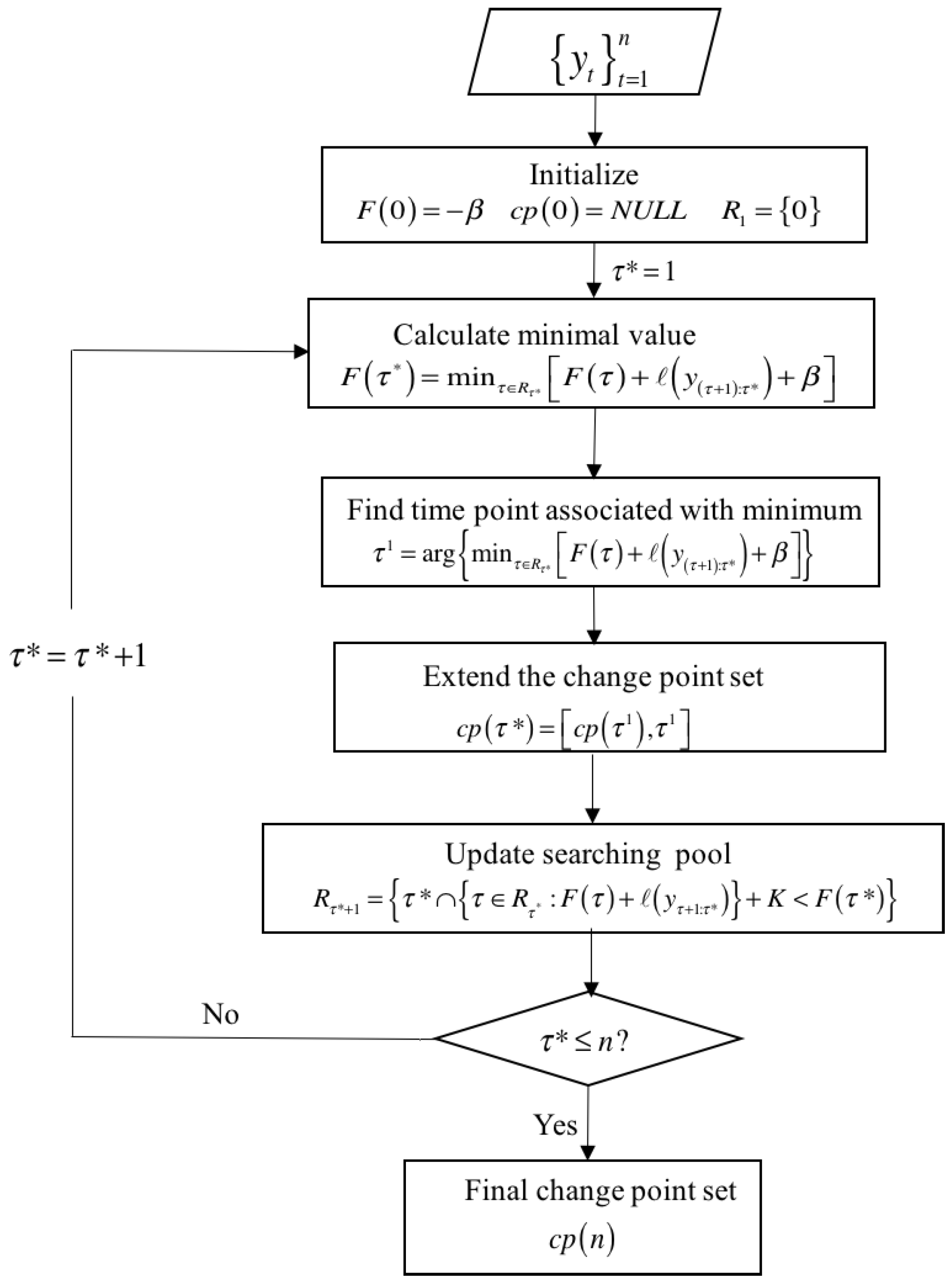
In above formulations, if the cost function is represented by negative log-likelihood, K = 0. The overview of the PELT algorithm is shown in Figure 1. We first initialize the objective function = and define an empty changepoint set and a searching pool. Second, we iteratively find the minimal value of objective function and associated time point , extend the change point set, and prune s that cannot reach optima by shrinking the searching pool . The pruning step shown in Figure 1 can significantly reduce the computational cost of the optimal partitioning approach especially when n is large.
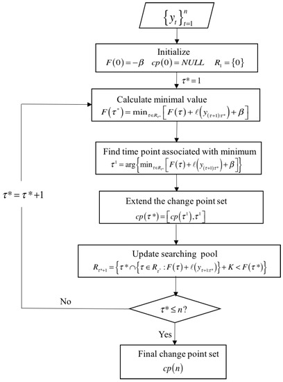
Figure 1.
Pruned exact linear time (PELT) algorithm overview.
2.2. Time Series Kalman Filter (TSKF)
Given a univariate data set , steps of an offline implementation of TSKF are as follows [23]:
- Data partition: partition the data set into M subsets .
- Pre-whitening: for each subset , pre-whiten the data using the reweighed minimum covariance determinant estimator [16], and centralize the data with robust center .
- Model fitting: based on the preliminary clean data ,
- 3.1.
- (Optional) select the model order p according to Bayesian information criteria [32].
- 3.2.
- Calculate the model coefficients based on Burg’s parameter estimation method [24].
- Outlier detection: for each subset :
- 4.1
- Reformat:where
- 4.2
- Predict:
- 4.3
- Update:
- 4.4
- Detect:
- 4.4.1.
- Set .
- 4.4.2.
- Find a number of n observations whose Mahalanobis distance .
- 4.4.3.
- Calculate the percentage of normal data:
- 4.4.4.
- If , stop; otherwise, increase by .
- 4.4.5.
- The outliers correspond to observations with Mahalanobis distance .
- 4.5
- Replace: replace the outliers with neighboring normal values.
Usually, the autoregressive model order will suffice, and, in this study, we pick the threshold , which means that we assume that the maximum amount of outliers in datasets would not exceed 5% of the total number of observations.
2.3. An Integrated Method for Outlier Detection in a Dynamic Data Set with Multiple Operating Points
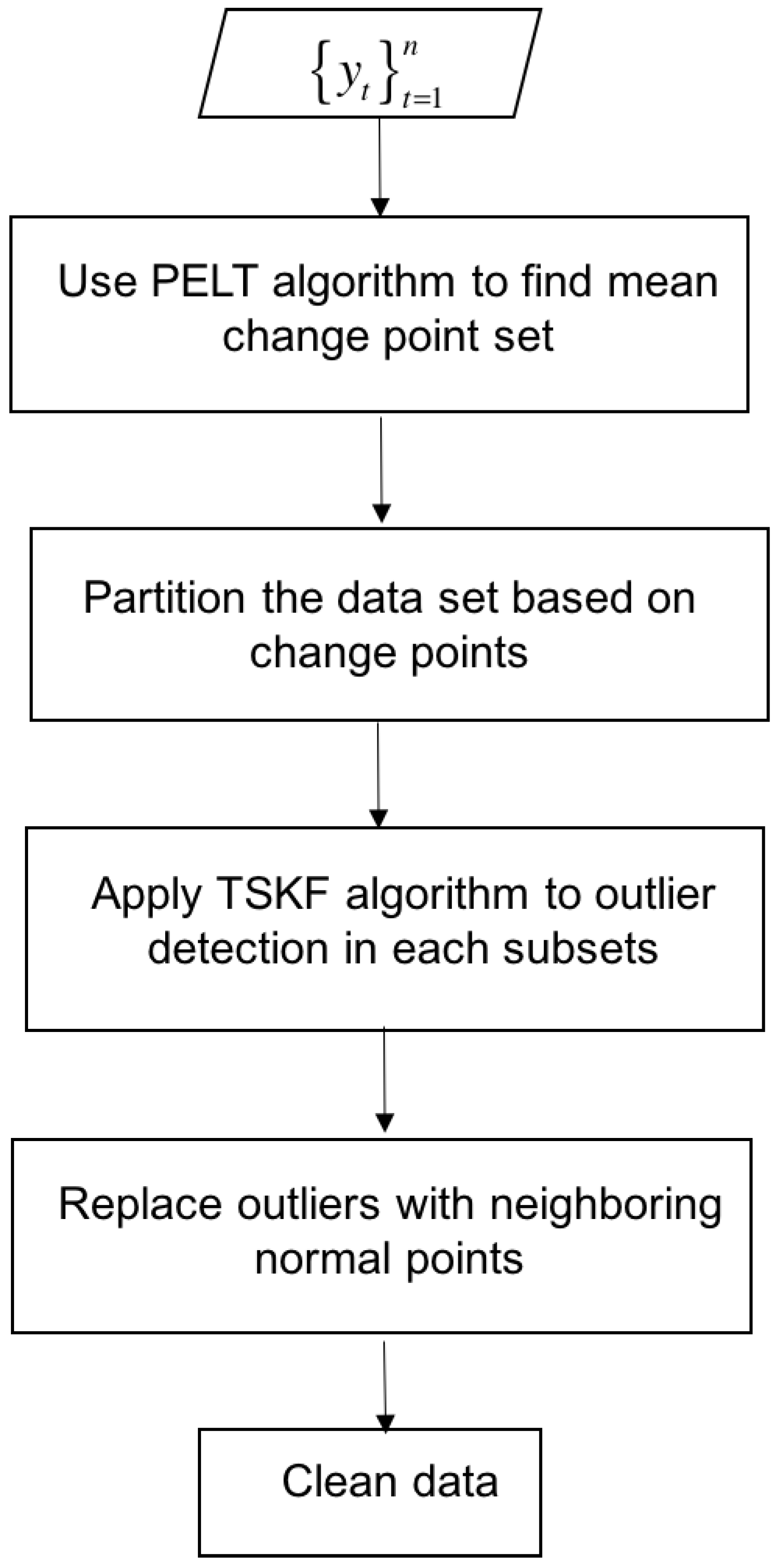
To overcome the challenge of outlier detection in dynamic data sets with multiple operating points, we propose to combine the PELT with TSKF, and an integrated methodology overview is shown in Figure 2. For each variable , we first use the PELT algorithm to find mean change points that segment the data and then apply TSKF to outlier detection within each subset bracketed by change points. Finally, we replace the outliers with neighboring normal points.
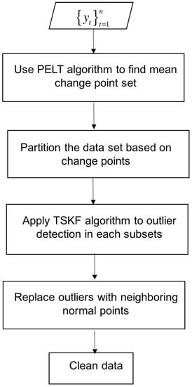
Figure 2.
An integrated outlier detection algorithm overview.
2.4. Partial Least Squares Discriminant Analysis (PLS-DA)
Partial least squares discriminant analysis (PLS-DA) is a linear classification method that derives from partial least squares (PLS) [33,34] by building a regression model between the predictor matrix and the predicted label matrix [35]. The standard mathematical formula for PLS-DA model is shown in Equation (20):
where is an matrix of predictors; is an one hot encoded matrix of class labels, and represents the membership of the i-th sample to the j-th class expressed with binary code (1 or 0); and are score matrices; and are and orthogonal loading matrices, respectively; and are error matrices assumed to be independently and identically distributed; are the regression coefficients.
A distinctive feature of PLS-DA is that it maximizes the covariance between and for each principal component spanning the reduced space, i.e., the covariance between and . In addition, advantages of PLS-DA include dimension reduction by using latent variables that are linear combinations of the original variables to model data variability and providing intuitive graphical visualization of data patterns and relations based on scores and loadings [36]. The PLS1 algorithm is commonly used to build PLS-DA models [37] in the two-class scenarios. PLS-DA returns estimated class values within (0,1). The classification of samples is conducted by choosing a label with the highest probability, and usually a threshold is used to determine which class a sample belongs to. In two-class scenarios with labels “0” and “1”, we assume that such a threshold equals 0.5 for simplicity, although the Bayes theorem can be used to give a more rigorous result [38].
3. Case Studies
In this section, PELT-TSKF’s capability of detecting univariate outliers in the dynamic data sets with multiple operating points is tested in simulated cases, and is compared with the general ESD (GESD) identifier [13] that detects outliers based on mean and standard deviation, and the isolation forest [22] that detects outliers based on finding points associated with the shortest average path lengths from the root node to the leaf node of a tree over the forest. (Note: the isolation forest is implemented in publicly available python package scikit-lean [39].). Moreover, we use an open-source sediment toxicity detection challenge as a toy problem to demonstrate the efficacy of PELT-TSKF in improving the PLS-DA model performance before applying the same methodology to industrial flare monitoring.
3.1. Simulated Case Study
In our simulated case studies, to illustrate the capability of outlier detection in dynamic data sets with mean shifts, performance of the new PELT-TSKF algorithm is compared with that of a GESD identifier combined with the PELT algorithm (the performance of GESD identifier will become much worse if without PELT). The intrinsic dynamic variation is approximated by a stationary autoregressive moving average (ARMA) (1,1) model:
where , are coefficients, is the white noise, and is a shift operator.
A total number of 1000 samples are simulated with two mean shifts at the 300th time point () and the 600th time point (), respectively.
The contamination rate is defined as the percentage of outliers in the data:
In our simulation case, , and outliers with equal probabilities being +Amp or −Amp (Amp is the amplitude of outliers) are added every 20th sample point except for the mean shift at the 300th and 600th time points.
The detection rate is defined as the percentage of outliers being successfully identified, and mis-identification rate is defined as the percentage of normal data falsely tagged as outliers (type I error):
A series of data sets with different values of are simulated repetitively 100 times each, and the average detection rate and mis-identification are given in Table 1.

Table 1.
Additive outlier detection results for data from autoregressive moving average (ARMA) (1, 1) multistage processes at .
Comparing the values of in Table 1, we can see that the PELT-TSKF works better than PELT-ESD and isolation forest algorithms when process autocorrelation increases with larger values of . The result suggests that system dynamics negatively affect the GESD identifier and isolation forest significantly.
Moreover, a larger outlier size Amp will surely help the outlier detection by increasing the outlier detection rate , but it will not necessarily decrease the mis-identification rate for PELT-GESD because the relative conservativeness of the GESD identifier leading to minor changes of the false alarms with different outlier sizes. Although the PELT-TSKF is generally more aggressive than the PELT-GESD with a higher mis-identification rate , it has limited influence when abundant data are available coming from high-frequency sampling.
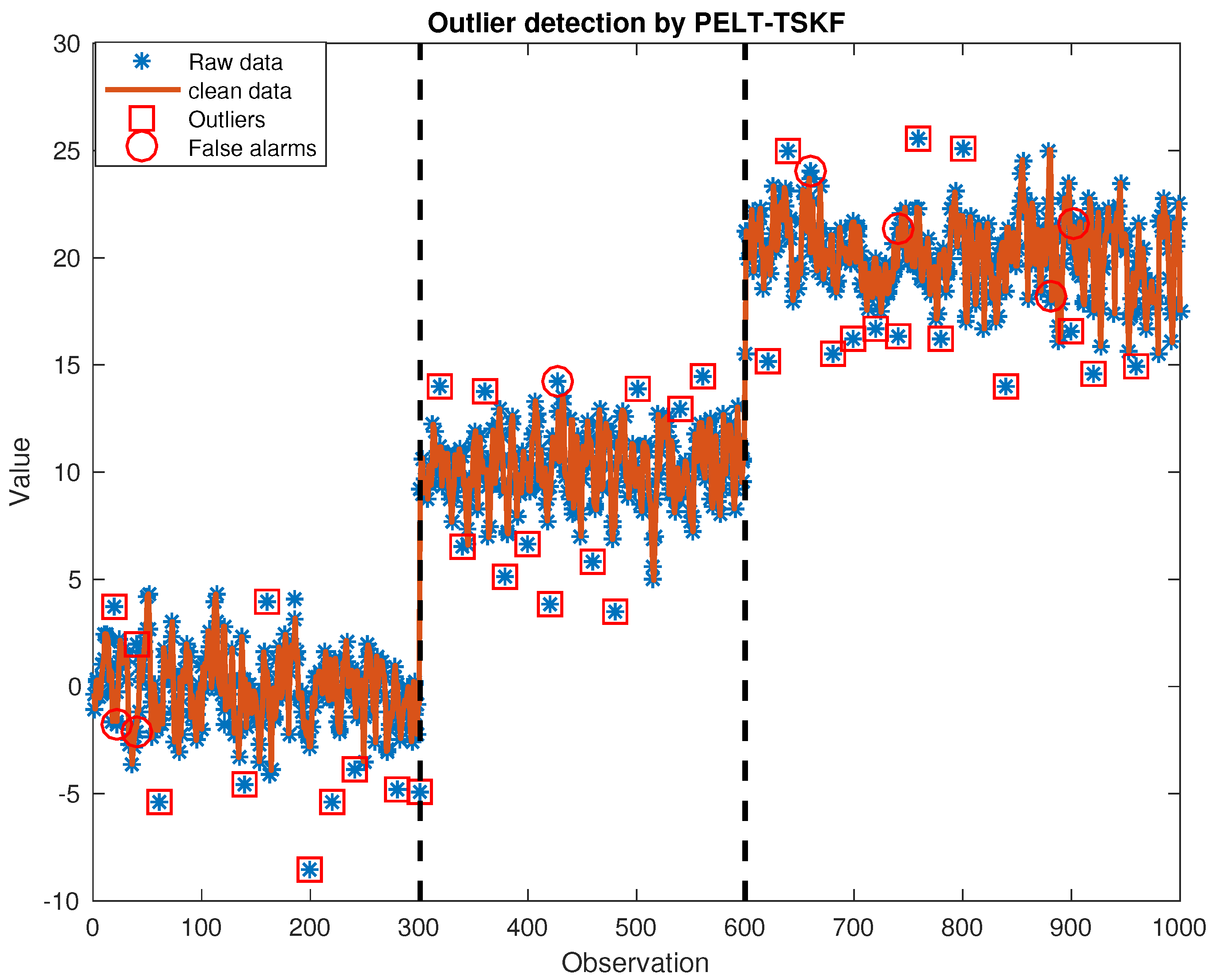
We provide an illustrative data set with , , . Figure 3 and Figure 4 show that the PELT algorithm can easily find two mean shifts at the 300th and 600th sample points marked by black dashed lines in both figures. In addition, additive outliers detected are highlighted by red squares, and we can see that the PELT-TSKF method is able to detect more additive outliers than the PELT-GESD identifier because there are more red squares in Figure 3 than in Figure 4. However, as indicated by the red circles shown in Figure 3, the PELT-TSKF cannot shield normal observations from swamping effects caused by outliers and leads to a few mis-identified instances—for example, the 21st point after an outlier at the 20th, and the 741st point after an outlier at the 740th time point are both mistaken for outliers because of previous anomalies.
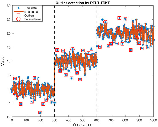
Figure 3.
Outlier detection by pruned exact linear time—time series Kalman filter (PELT-TSKF).
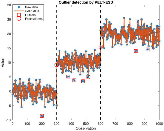
Figure 4.
Outlier detection by pruned exact linear time—general extreme studentized deviate (PELT-GESD).
3.2. Application of PELT-TSKF to PLS-DA Case Studies
3.2.1. Sediment Toxicity Detection
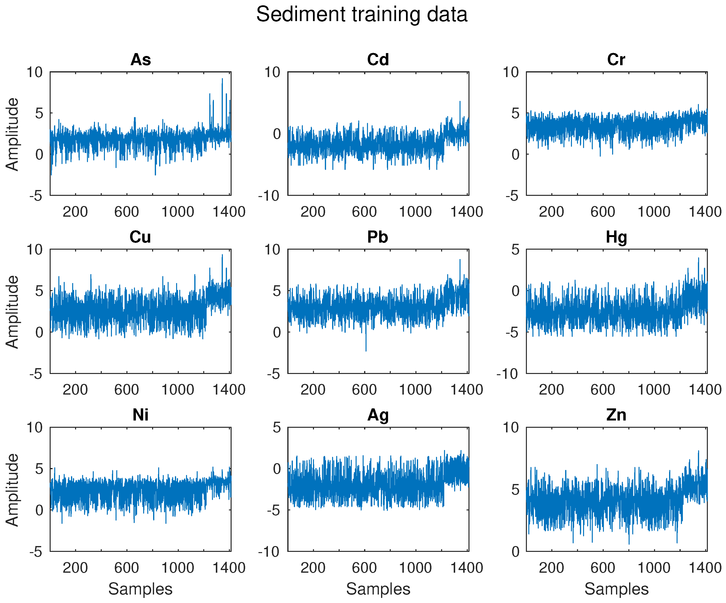
In this section, a sediment dataset is used. The data include 1884 sediment samples and nine chemical variables that are the log-transformed concentrations (ppm) of metals (As, Cd, Cr, Cu, Pb, Hg, Ni, Ag, Zn) [40]. Sediment samples are divided into two classes on the basis of their toxicity, as shown in Table 2. While class 1 contains 1624 non-toxic samples, class 2 includes 260 toxic samples.
Table 2.
Sediment dataset: sample partition in toxic and non-toxic classes.
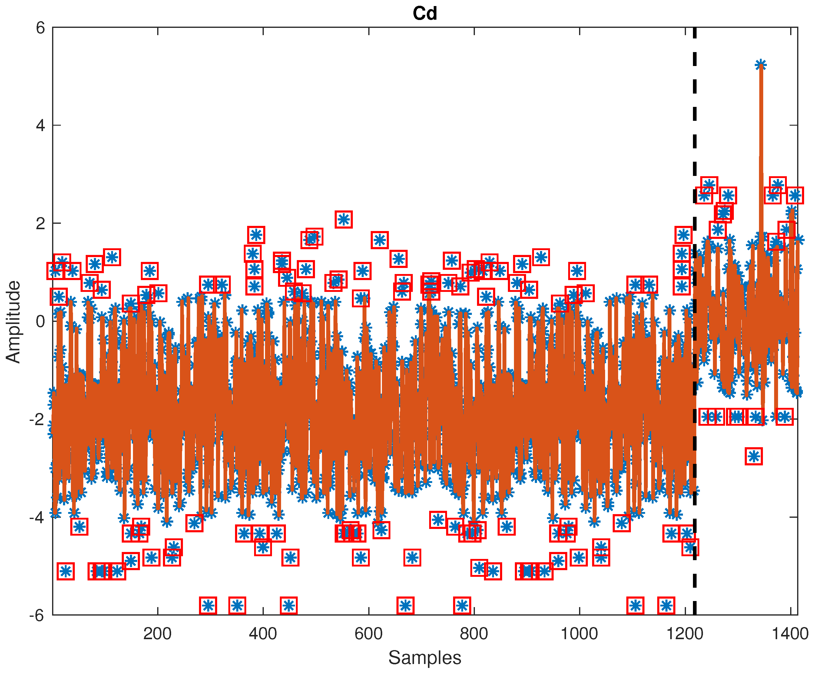
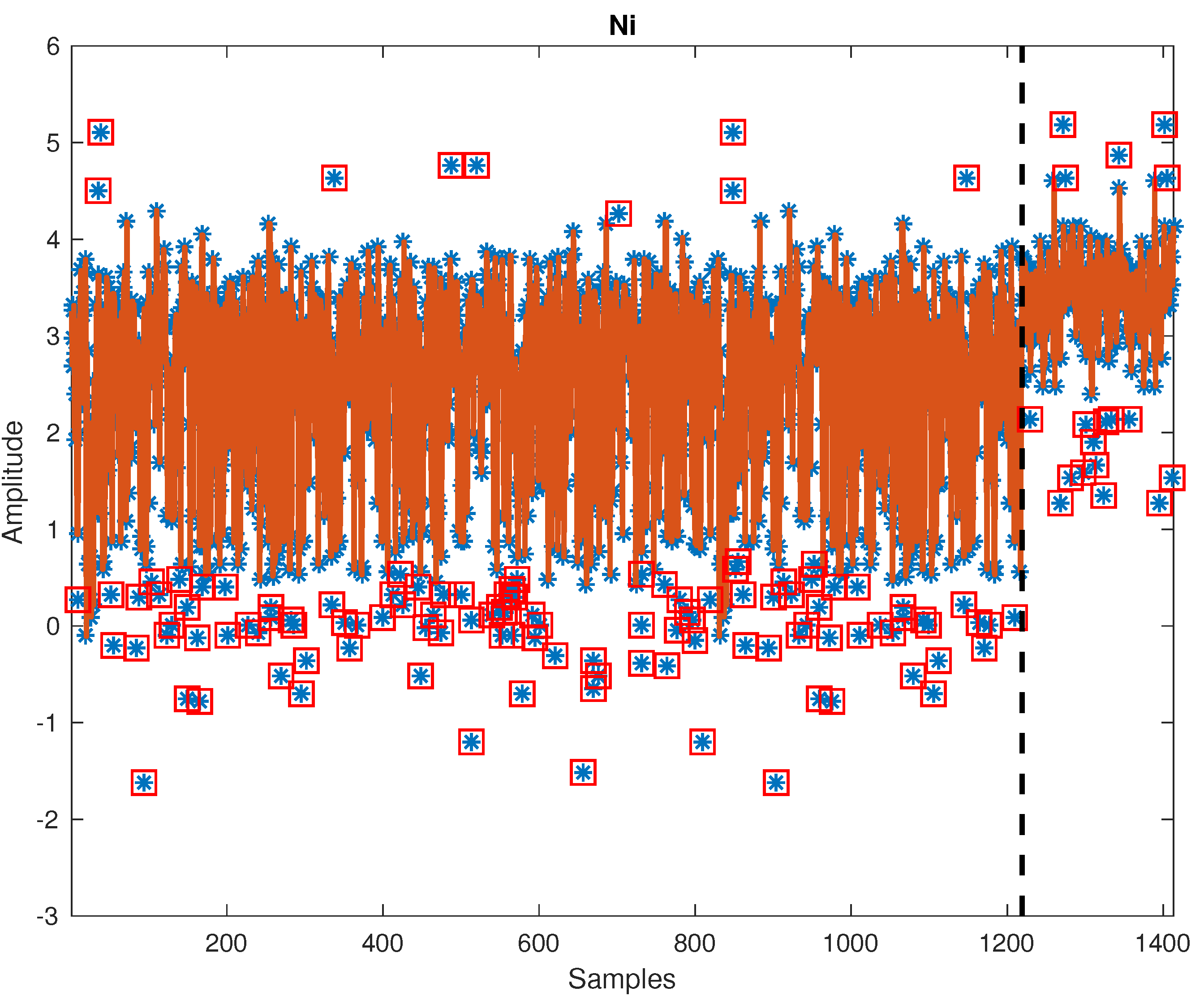
Figure 5 displays raw training of the sediment data set. There are obvious mean shifts in variables like Cd, Cu, Ni, Ag, and Zn. Figure 6 and Figure 7 show cleaning results by PELT-TSKF on Cd and Ni data set. The new method is able to detect abnormal observations highlighted in red squares and find the mean shift points marked by black dash lines. In Figure 6, there is still an outlier at around the 1300th point that the PELT-TSKF fails to detect, mainly because there are not enough normal data on the second stage to provide a good estimation of autoregressive models. As a result, the outlier detection performance is compromised.
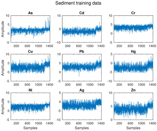
Figure 5.
Sediment training data set.
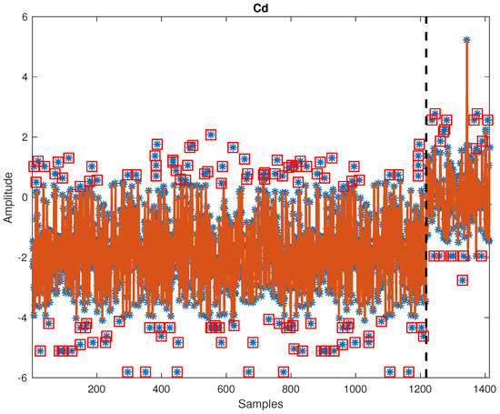
Figure 6.
Outlier detection result on Cd.

Figure 7.
Outlier detection result on Ni.
Both raw training and testing data sets are cleaned by PELT-TSKF. Then, raw and clean data sets are both weight centered by subtracting the average means of two groups to remove biases caused by unequal class sizes [37] and scaled using associated standard deviations. PLS-DA models are built and tested based on resulting standardized raw and clean data sets. Three principal components are selected based on cross-validation and are able to capture 80% of total variance of .
Three metrics are used to evaluate the model performance: non-error rate (NER, percentage of correctly predicted samples), toxicity sensitivity (Sn, ability to correctly recognize toxic samples as toxic in percentage), and non-toxicity specificity (Sp, ability to correctly recognize non-toxic samples as non-toxic, in percentage). The model testing results are shown in Table 3:
Table 3.
Sediment test results summary.
Results in Table 3 show that cleaning the outliers by PELT-TSKF improved the data quality and consequently improved the PLS-DA classification results as reflected through three metrics: increased from 0.792 to 0.847, from 0.846 to 0.877 and from 0.783 to 0.842.
3.2.2. Industrial Flare Monitoring
In this section, the application of the proposed PELT-TSKF method and PLS-DA is tested with flare data sets taken from the petrochemical industry (for intellectual property reasons, the variables are named V1, V2, ...). Data are sampled at every 1 min. Flares associated with non-routine situations are tagged with “1” as opposed to those corresponding to normal operations with “0”. We randomly select two testing data sets and use observations that precede them as training data. Details on the sizes of training and testing sets are listed in Table 4.
Table 4.
Sizes of training and testing sets.
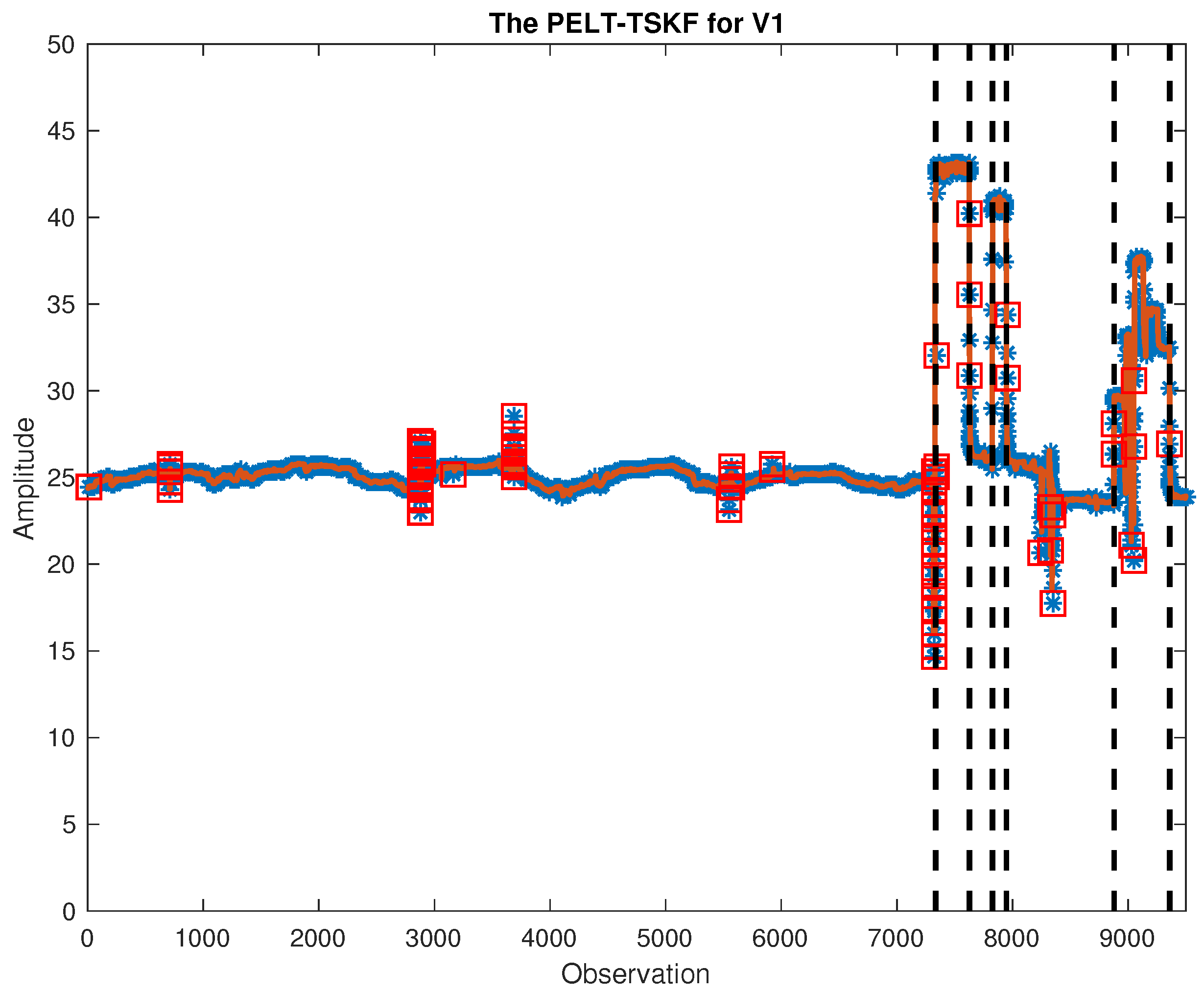
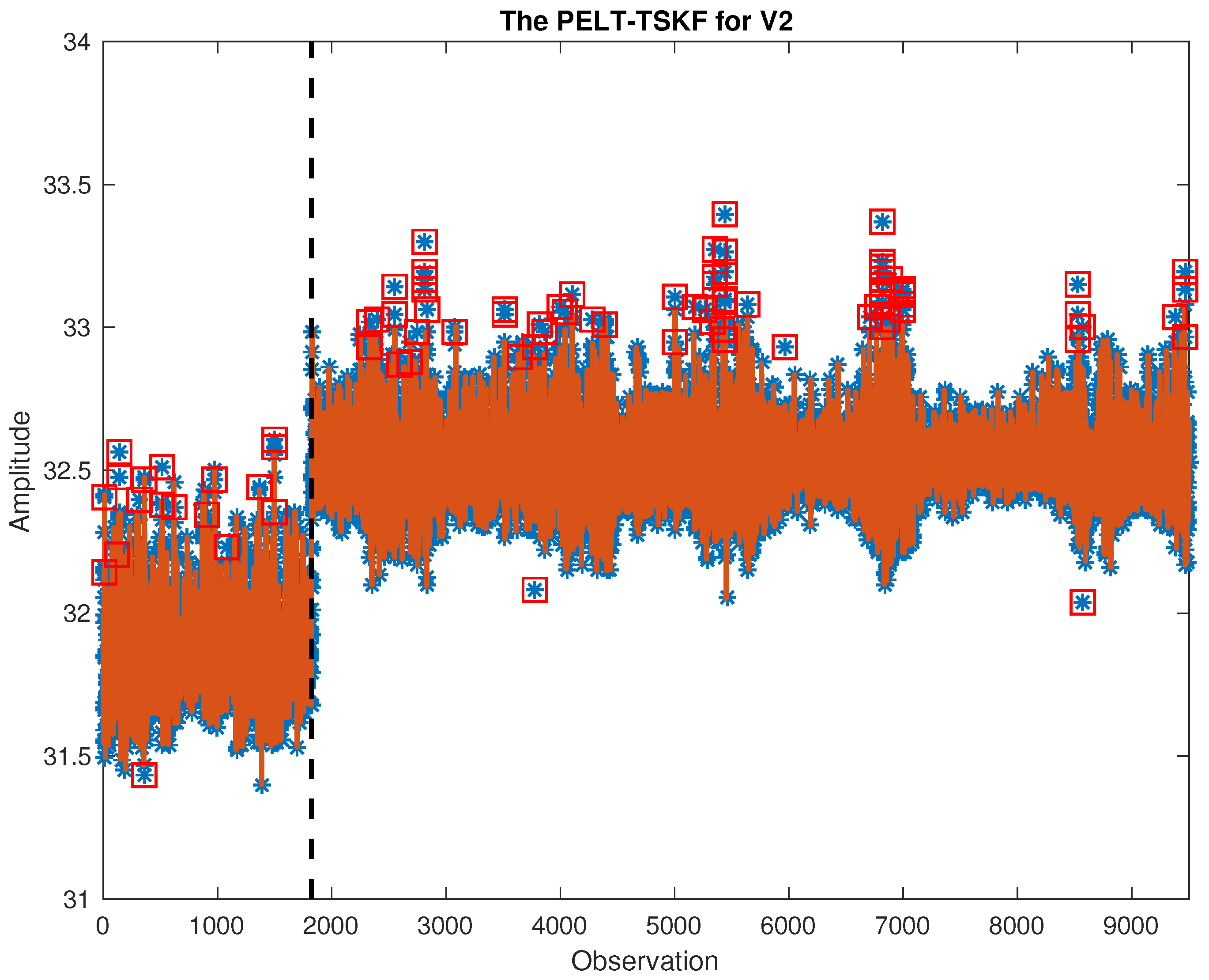
In this study, out of 132 variables, we focus on critical ones including feed/outlet flows, temperature, water level, etc. Critical variables in both training and testing data are cleaned using PELT-TSKF methods, and part of the results are shown in Figure 8 and Figure 9. As highlighted by black dash lines and red squares, the new algorithm is able to find out mean shift points while detecting outliers masked by process variations.
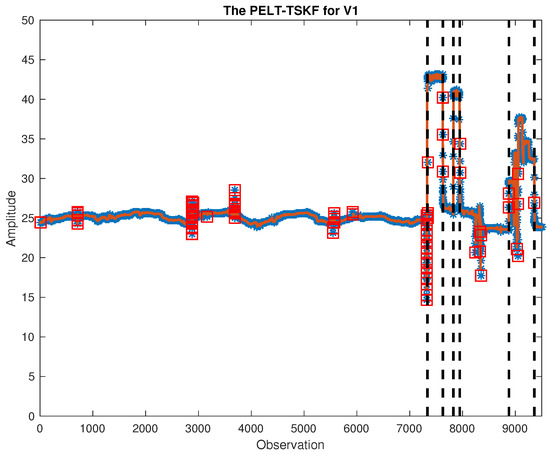
Figure 8.
PELT-TSKF for V1.
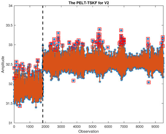
Figure 9.
PELT-TSKF for V2.
Two metrics are used to evaluate the performance of non-routine flares detection: detection rate and false alarm rate :
Table 5 summarizes PLS-DA results based on raw and clean flare data sets, and we can see that cleaning outliers improves flare monitoring results in the Flare 1 case, increasing the detection rate from 62.86% to 88.47%. In addition, although removing outliers does not affect the false alarm rate in the Flare 1 case, it helps reduce false alarm rates in the Flare 2 case, decreasing the false alarm rate from 0.18% to 0.16% or reducing six false alarms in total.
Table 5.
Partial least squares-discriminant analysis (PLS-DA) results on raw and clean data sets.
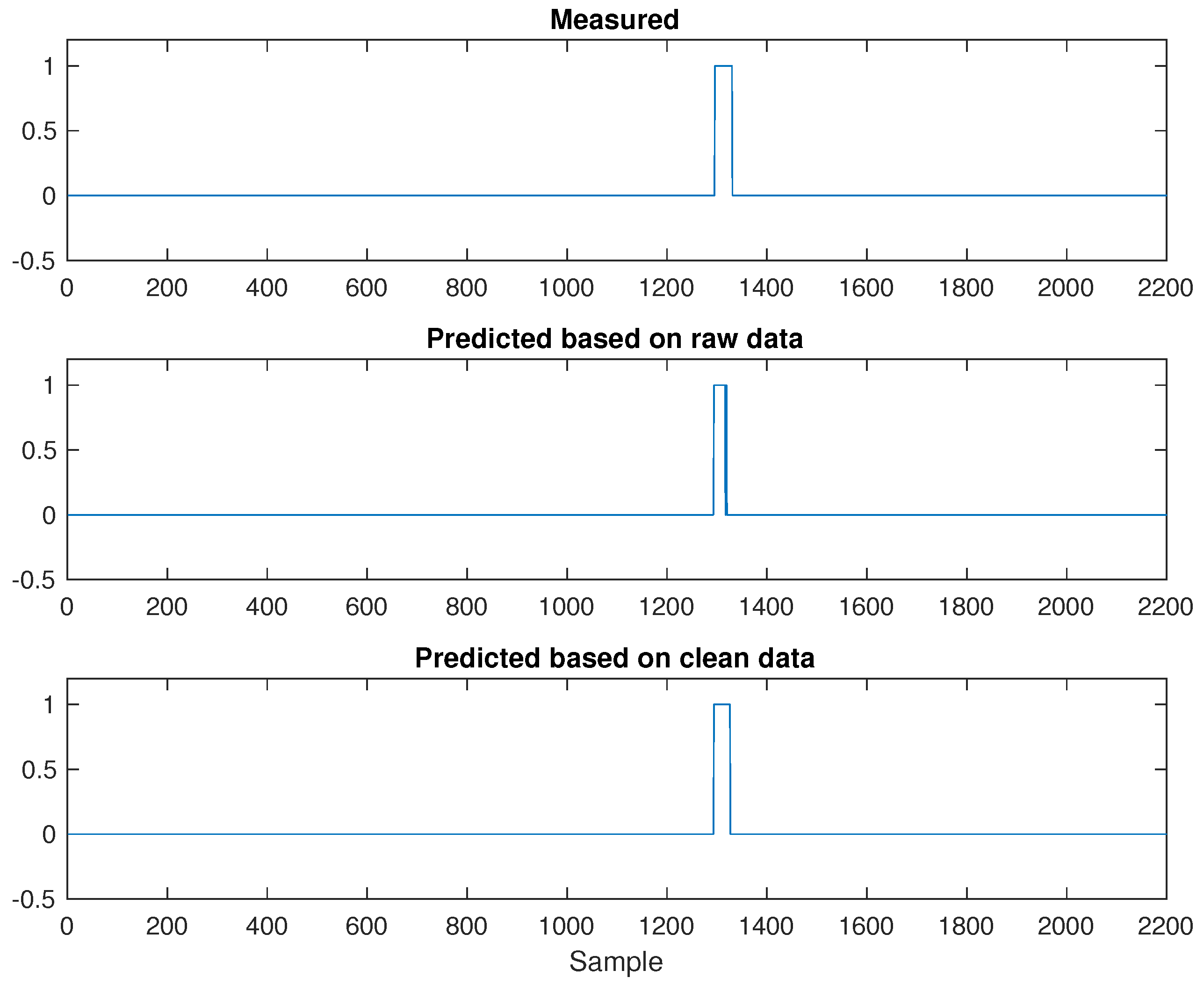
Furthermore, Figure 10 and Figure 11 illustrate flare monitoring results obtained from PLS-DA models built on raw and clean data sets. While Y = 1 indicates the occurrence of non-routine flares, Y = 0 represents normal operation. Regarding Flare 1 results, comparing the middle plot with the bottom one shown in Figure 10, we can see that cleaning outliers will slightly increase the width of rectangular pulse, leading to a flare detection result close to the true measured flare events given by the plot on top.
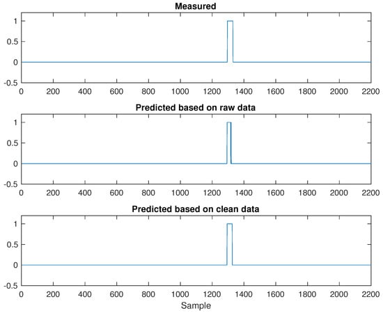
Figure 10.
Flare 1: Partial least squares-discriminant analysis (PLS-DA) based on raw and clean data.
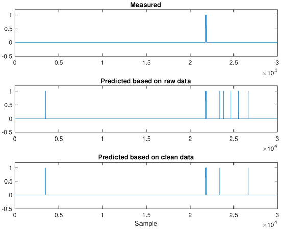
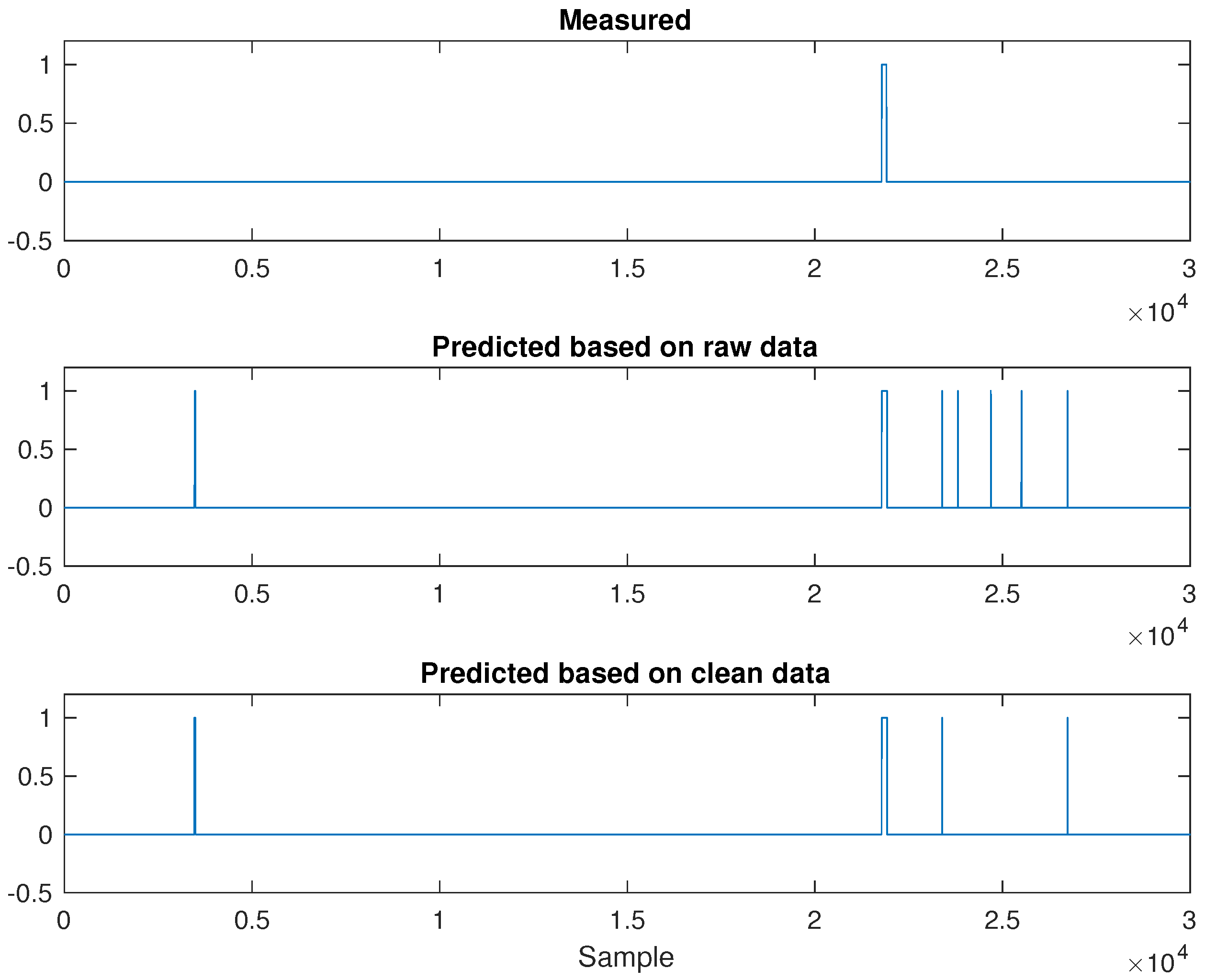
Figure 11.
Flare 2: PLS-DA analysis based on raw and clean data.
As for Flare 2 results in Figure 11, we can easily find out that there are more spikes shown in the middle plot associated with raw data than the bottom one corresponding to a clean data set, indicating that the plant will suffer from a larger false alarm rate if no data cleaning is applied.
4. Discussion
From the results of simulated ARMA (1,1) data with mean shifts, we can see that PELT-TSKF is able to correctly identify the two stage changes and outperformed the general ESD and isolation forest approaches in outlier identification accuracy. This is especially apparent when the process dynamics become significant (shown by larger autocorrelation coefficients). However, it is worth pointing out that the isolation forest can also be used to identify multivariate outliers and is more efficient than the extension of TSKF in multivariate cases. The toy problem of sediment toxicity detection illustrates a successful application of PELT-TSKF in practice: cleaning outliers from concentration measurements and increasing the non-error rate, toxicity sensitivity and non-toxicity specificity calculated from the PLS-DA model as a result. In the flare monitoring case study, on the one hand, we demonstrate that applying data-driven approaches like PLS-DA can effectively assist process engineers; on the other hand, the efficacy of new PELT-TSKF has been proved in ameliorating the quality of industrial flaring data which contain multiple operating points, and improving the resulting flare monitoring performance by increasing the anomaly detection rate and reducing possibilities of false alarms.
5. Conclusions
Taking advantage of abundant raw plant data gathered by intelligent devices plays an important role in transforming modern plant operations from reactive to predictive. Data cleaning lays the foundation of knowledge discovery from data. In this paper, we focus on overcoming the challenges of outlier detection in dynamic systems with multiple operating points, and propose a novel method combining the time series Kalman filter (TSKF) with the pruned exact linear time (PELT) approach. The PELT-TSKF approach is able to pinpoint mean shifts and differentiate outliers from process variations at the same time. In addition, we demonstrate that applying data driven PLS-DA can assist process engineers in flare monitoring, and cleaning outliers using TSKF-PELT can further improve the performance of such a challenge task.
Although our method is able to deal with univariate outlier detection within dynamic system mean shifts, in practice, process operating points may be characterized by other factors other than mean, such as variance or frequency. In addition, operating point changes may affect individual variables in different ways: while a few of them show mean shifts, others exhibit variance changes. In addition, we only consider situations where operating point changes are significant enough that the impact of outliers can be ignored. When the impact of outliers on change points detection becomes significant, we can apply cross-validation to determine the optimal number of stage changes associated with the lowest cross validation error. Furthermore, multivariate outliers are also usually faced in process data, and how to efficiently detect multivariate outliers in the dynamic systems with multiple operating points is worth exploring in the future.
Acknowledgments
The authors would like to gratefully acknowledge the financial and technical support from the Emerson Process Management.
Author Contributions
Shu Xu and Bo Lu designed case studies; Shu Xu conducted the case studies, analyzed the data and wrote the paper; Noel Bell and Mark Nixon provided the industrial flare monitoring data and provided feedback on the results.
Conflicts of Interest
The authors declare no conflict of interest.
Abbreviations
The following abbreviations are used in this manuscript:
| TSKF | time series Kalman filter |
| PELT | pruned exact linear time |
| PLS-DA | partial least squares discriminant analysis |
| GESD | general extreme studentized deviate |
| ARMA | autoregressive moving average |
| NER | non-error rate |
| Sn | toxicity sensitivity |
| Sp | non-toxicity specificity |
References
- Davis, J.; Edgar, T.; Porter, J.; Bernaden, J.; Sarli, M. Smart manufacturing, manufacturing intelligence and demand-dynamic performance. Comput. Chem. Eng. 2012, 47, 145–156. [Google Scholar] [CrossRef]
- Torres, V.M.; Herndon, S.; Kodesh, Z.; Allen, D.T. Industrial flare performance at low flow conditions. 1. study overview. Ind. Eng. Chem. Res. 2012, 51, 12559–12568. [Google Scholar] [CrossRef]
- Bader, A.; Baukal, C.E., Jr.; Bussman, W. Selecting the proper flare systems. Chem. Eng. Prog. 2011, 107, 45–50. [Google Scholar]
- Xu, S.; Lu, B.; Baldea, M.; Edgar, T.F.; Wojsznis, W.; Blevins, T.; Nixon, M. Data cleaning in the process industries. Rev. Chem. Eng. 2015, 31, 453–490. [Google Scholar] [CrossRef]
- Hodge, V.J.; Austin, J. A survey of outlier detection methodologies. Artif. Intell. Rev. 2004, 22, 85–126. [Google Scholar] [CrossRef]
- Daszykowski, M.; Kaczmarek, K.; Heyden, Y.V.; Walczak, B. Robust statistics in data analysis—A review: Basic concepts. Chemometr. Intell. Lab. Syst. 2007, 85, 203–219. [Google Scholar] [CrossRef]
- Singh, A. Outliers and robust procedures in some chemometric applications. Chemometr. Intell. Lab. Syst. 1996, 33, 75–100. [Google Scholar] [CrossRef]
- Dielman, T.E. Least absolute value regression: Recent contributions. J. Stat. Comput. Simul. 2005, 75, 263–286. [Google Scholar] [CrossRef]
- Jaeckel, L.A. Estimating regression coefficients by minimizing the dispersion of the residuals. Ann. Math. Stat. 1972, 43, 1449–1458. [Google Scholar] [CrossRef]
- Huber, P.J. Robust estimation of a location parameter. Ann. Math. Stat. 1964, 35, 73–101. [Google Scholar] [CrossRef]
- Rousseeuw, P.; Yohai, V. Robust regression by means of S-estimators. In Robust and Nonlinear Time Series Analysis; Springer-Verlag: New York, NY, USA, 1984; pp. 256–272. [Google Scholar]
- Davies, L.; Gather, U. The identification of multiple outliers. J. Am. Stat. Assoc. 1993, 88, 782–792. [Google Scholar] [CrossRef]
- Rosner, B. Percentage points for a generalized ESD many-outlier procedure. Technometrics 1983, 25, 165–172. [Google Scholar] [CrossRef]
- Hampel, F.R. A general qualitative definition of robustness. Ann. Math. Stat. 1971, 42, 1887–1896. [Google Scholar] [CrossRef]
- Tukey, J.W. Exploratory Data Analysis (Behavior Science); Pearson: London, UK, 1977. [Google Scholar]
- Rousseeuw, P.J.; Driessen, K.V. A fast Algorithm for the minimum covariance determinant estimator. Technometrics 1999, 41, 212–223. [Google Scholar] [CrossRef]
- Allan, J.; Carbonell, J.; Doddington, G.; Yamron, J.; Yang, Y. Topic detection and tracking pilot study final report. In Proceedings of the DARPA Broadcast News Transcription and Understanding Workshop, Pittsburgh, PA, USA, 8–11 February 1998; pp. 194–218. [Google Scholar]
- Knorr, E.M.; Ng, R.T. Algorithms for mining distance based outliers in large datasets. In Proceedings of the International Conference on Very Large Data Bases; Gupta, A., Shmueli, O., Widom, J., Eds.; Morgan Kaufmann: New York, NY, USA, 1998; pp. 392–403. [Google Scholar]
- Tax, D.M.J.; Duin, R.P.W. Support vector data description. Mach. Learn. 2004, 54, 45–66. [Google Scholar] [CrossRef]
- Chiang, L.H.; Russell, E.L.; Braatz, R.D. Fault Detection and Diagnosis in Industrial Systems; Springer-Verlag: London, UK, 2001. [Google Scholar]
- Kourti, T.; MacGregor, J.F. Process analysis, monitoring and diagnosis, using multivariate projection methods. Chemometr. Intell. Lab. Syst. 1995, 28, 3–21. [Google Scholar] [CrossRef]
- Liu, F.T.; Ting, K.M.; Zhou, Z.H. Isolation Forest. In Proceedings of the ICDM Conference, Pisa, Italy, 15–19 December 2008. [Google Scholar]
- Xu, S.; Baldea, M.; Edgar, T.F.; Wojsznis, W.; Blevins, T.; Nixon, M. An improved methodology for outlier detection in dynamic datasets. AIChE J. 2015, 61, 419–433. [Google Scholar] [CrossRef]
- Kay, S.M. Modern Spectral Estimation: Theory and Application; Prentice Hall: Bergen County, NJ, USA, 1988. [Google Scholar]
- Dunia, R.; Edgar, T.F.; Blevins, T.; Wojsznis, W. Multistate analytics for continuous processes. J. Process Control 2012, 22, 1445–1456. [Google Scholar] [CrossRef]
- Killick, R.; Fearnhead, P.; Eckley, I.A. Optimal detection of changepoints with a linear computational cost. J. Am. Stat. Assoc. 2012, 107, 1590–1598. [Google Scholar] [CrossRef]
- Jackson, B.; Sargle, J.D.; Barnes, D.; Arabhi, S.; Alt, A.; Gioumousis, P.; Gwin, E.; Sangtrakulcharoen, P.; Tan, L.; Tsai, T.T. An algorithm for optimal partitioning of data on an interval. IEEE Signal Process. Lett. 2005, 12, 105–108. [Google Scholar] [CrossRef]
- Scott, A.J.; Knott, M. A cluster analysis method for grouping means in the analysis of variance. Biometrics 1974, 30, 507–512. [Google Scholar] [CrossRef]
- Auger, I.E.; Lawrence, C.E. Algorithms for the optimal identification of segment neighborhoods. Bull. Math. Biol. 1989, 51, 39–54. [Google Scholar] [CrossRef] [PubMed]
- Adams, R.P.; MacKay, D.J.C. Bayesian Online Changepoint Detection. 2007. Available online: http://arxiv.org/abs/0710.3742 (accessed on 3 March 2017).
- Lai, T.L.; Xing, H. Sequential Change-Point Detection When the Pre- and Post-Change Parameters are Unknown. Seq. Anal. 2010, 29, 162–175. [Google Scholar] [CrossRef]
- Schwarz, G. Estimating the dimension of a model. Ann. Stat. 1978, 6, 461–464. [Google Scholar] [CrossRef]
- Geladi, P.; Kowalski, B.R. Partial least squares: A tutorial. Anal. Chim. Acta 1986, 185, 1–17. [Google Scholar] [CrossRef]
- Wold, S.; Sjostrom, M.; Eriksson, L. PLS-regression: A basic tool of chemometrics. Chemom. Intell. Lab. Syst. 2001, 58, 109–130. [Google Scholar] [CrossRef]
- Brereton, R.G. Chemometrics for Pattern Recognition; John Wiley and Sons: Chichester, UK, 2009. [Google Scholar]
- Ballabio, D.; Consonni, V. Classification tools in chemistry. Part 1: Linear models. PLS-DA. Anal. Method 2013, 5, 3790–3798. [Google Scholar] [CrossRef]
- Brereton, R.G.; Lloyd, G.R. Partial least squares discriminant analysis: Taking the magic away. J. Chemom. 2014, 28, 213–225. [Google Scholar] [CrossRef]
- Pérez, N.F.; Ferré, J.; Boqué, R. Calculation of the reliability of classification in discriminant partial least-squares binary classification. Chemom. Intell. Lab. Syst. 2009, 95, 122–128. [Google Scholar] [CrossRef]
- Pedregosa, F.; Varoquaux, G.; Gramfort, A.; Michel, V.; Thirion, B.; Grisel, O.; Blondel, M.; Prettenhofer, P.; Weiss, R.; Dubourg, V.; et al. Scikit-learn: Machine Learning in Python. J. Mach. Learn. Res. 2011, 12, 2825–2830. [Google Scholar]
- Alvarez-Guerra, M.; Ballabio, D.; Amigo, J.M.; Viguri, J.R.; Bro, R. A chemometric approach to the environmental problem of predicting toxicity in contaminated sediments. J. Chemom. 2010, 24, 379–386. [Google Scholar] [CrossRef]

© 2017 by the authors. Licensee MDPI, Basel, Switzerland. This article is an open access article distributed under the terms and conditions of the Creative Commons Attribution (CC BY) license (http://creativecommons.org/licenses/by/4.0/).