Design of S2N—NEWMA Control Chart for Monitoring Process having Indeterminate Production Data


Abstract
:1. Introduction
2. Preliminaries and the Proposed Statistic
3. The Proposed Control Chart
- Step-1: Select a random sample of size from the industrial process and compute statistic .
- Step-2: Announce the process is shifted if or .
- Generate 10,000 random sample of size from neutrosophic normal distribution from the in-control process. Choose values of , , and from Table 1. Compute and plot them on and . Note first out-of-control and calculate their average.
- Compute and NSD and determine where , where are specified values of .
- Select those when very close to .
- Generate random sample of size from the shifted process. Compute and plot them on and . Note first out-of-control and calculate their average.
- Compute and NSD for a various shift .
4. Comparative Study
4.1. Advantage of the Proposed Chart in Neutrosophic Average Run Length (NARL) and Neutrosophic Standard Deviation (NSD)
4.2. Simulation Study
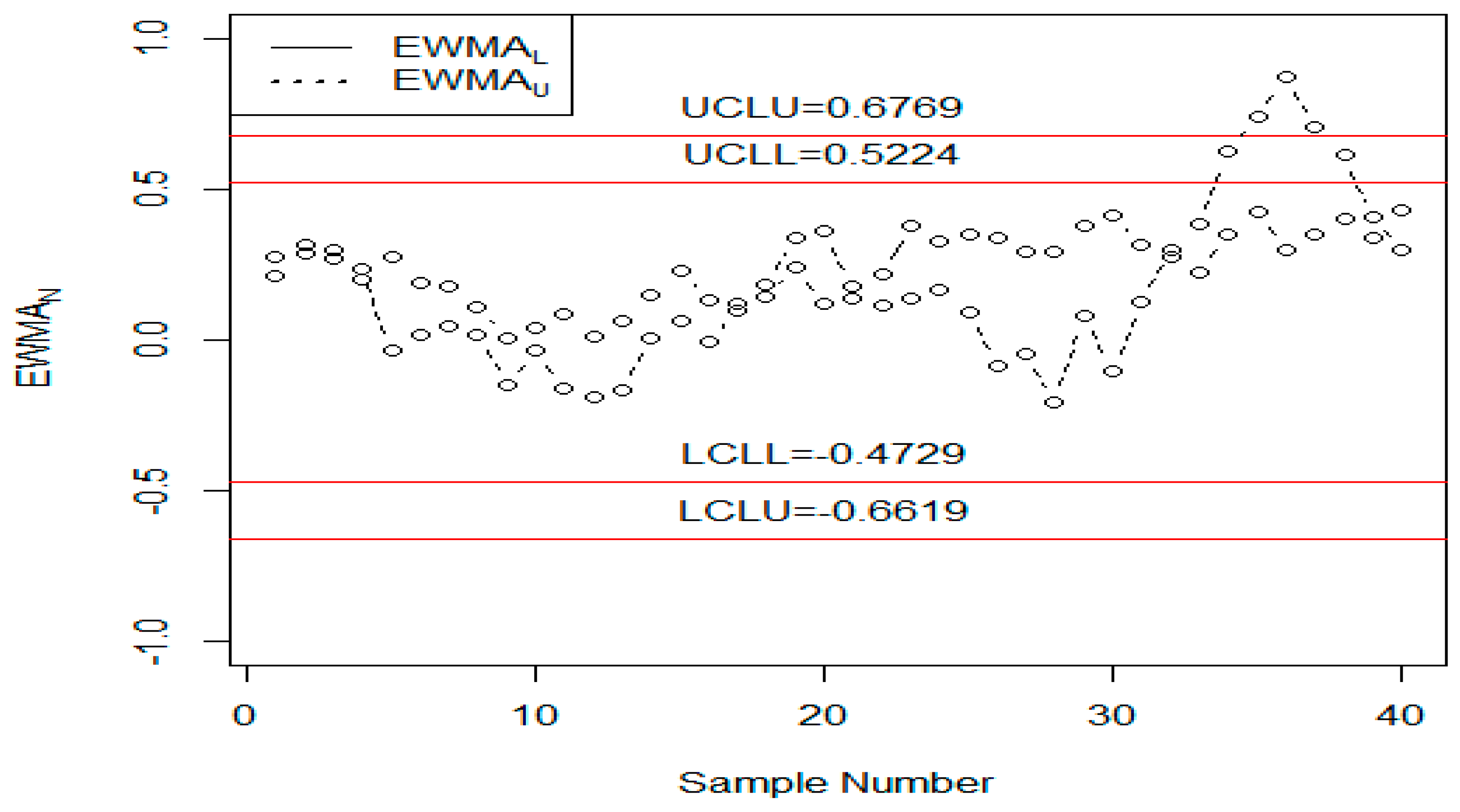
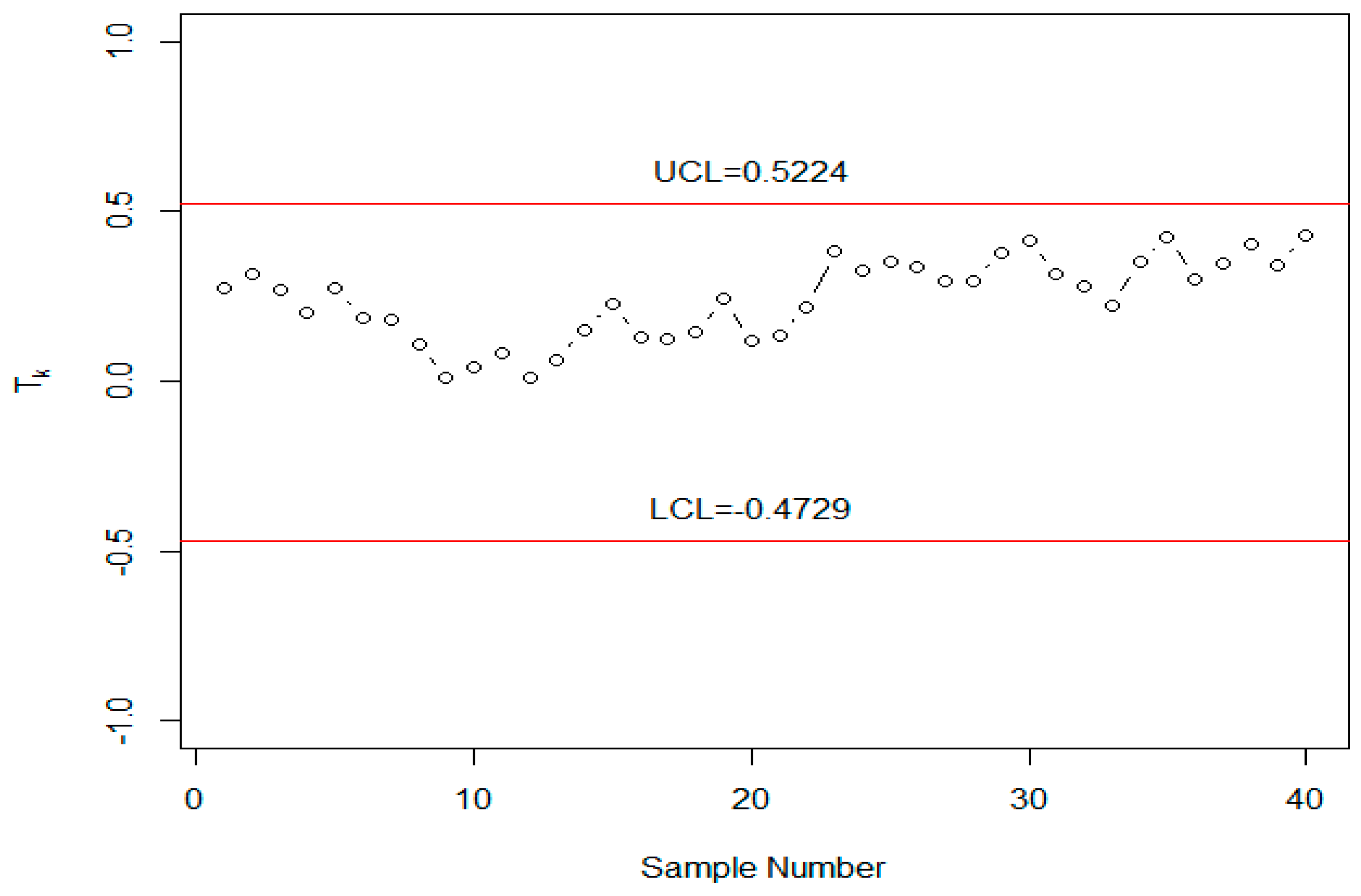
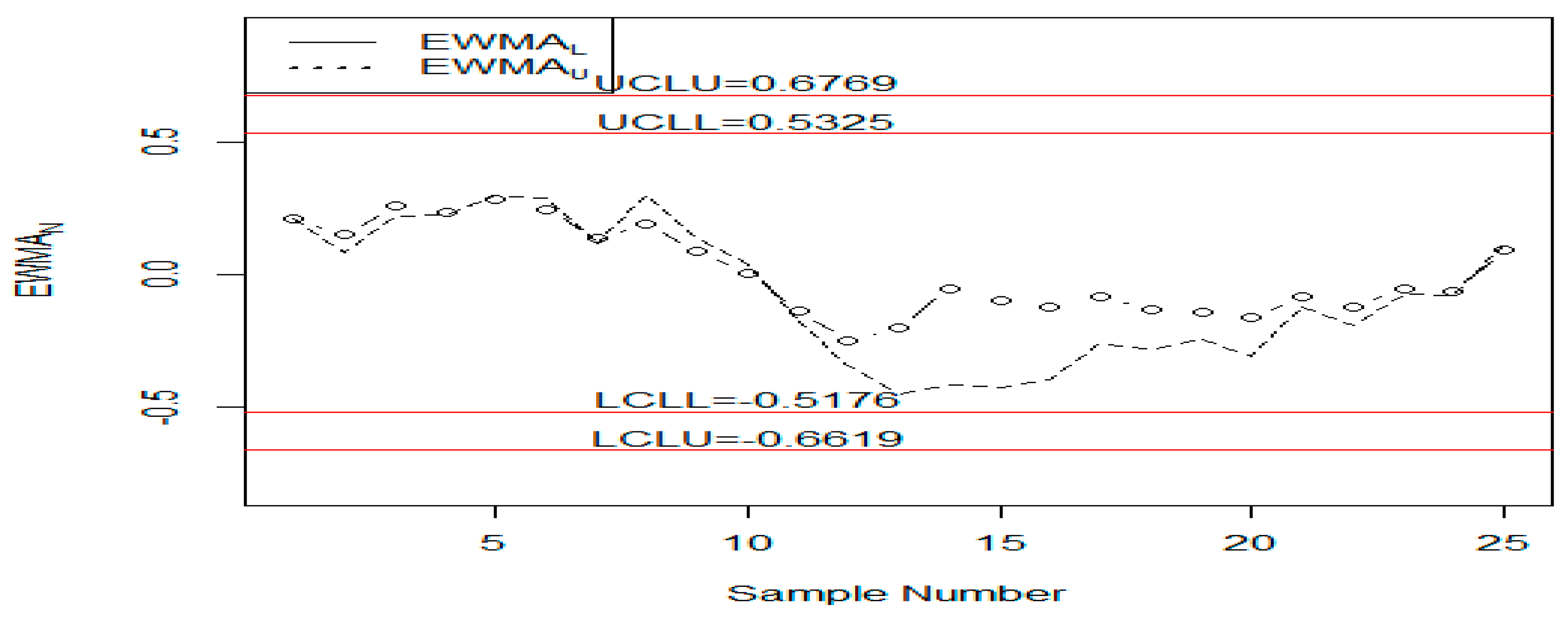
5. Application
6. Concluding Remarks
Author Contributions
Funding
Acknowledgments
Conflicts of Interest
References
- Aslam, M.; Khan, N.; Jun, C.-H. A new S 2 control chart using repetitive sampling. J. Appl. Stat. 2015, 42, 2485–2496. [Google Scholar] [CrossRef]
- Aslam, M.; Khan, N.; Albassam, M. Control chart for failure-censored reliability tests under uncertainty environment. Symmetry. 2018, 10, 690. [Google Scholar] [CrossRef]
- Azam, M.; Arshad, A.; Aslam, M.; Jun, C.-H. A control chart for monitoring the process mean using successive sampling over two occasions. Arab. J. Sci. Eng. 2017, 42, 2915–2926. [Google Scholar] [CrossRef]
- Prajapati, D.R.; Mahapatra, P.B. An effective joint X-bar and R chart to monitor the process mean and variance. Int. J. Product. Qual. Manag. 2007, 2, 459–474. [Google Scholar] [CrossRef]
- Aslam, M.; Rao, G.S.; Al-Marshadi, A.H.; Jun, C.-H. A Nonparametric HEWMA-p Control chart for variance in monitoring processes. Symmetry 2019, 11, 356. [Google Scholar] [CrossRef]
- Roberts, S. Control chart tests based on geometric moving averages. Technometrics 1959, 1, 239–250. [Google Scholar] [CrossRef]
- Castagliola, P. A new S2-EWMA control chart for monitoring the process variance. Qual. Reliab. Eng. Int. 2005, 21, 781–794. [Google Scholar] [CrossRef]
- Haq, A. An improved mean deviation exponentially weighted moving average control chart to monitor process dispersion under ranked set sampling. J. Stat. Comput. Simulat. 2014, 84, 2011–2024. [Google Scholar] [CrossRef]
- Haq, A.; Brown, J.; Moltchanova, E. New exponentially weighted moving average control charts for monitoring process mean and process dispersion. Qual. Reliab. Eng. Int. 2015, 31, 877–901. [Google Scholar] [CrossRef]
- Haq, A.; Brown, J.; Moltchanova, E.; Al-Omari, A.I. Effect of measurement error on exponentially weighted moving average control charts under ranked set sampling schemes. J. Stat. Comput. Simulat. 2015, 85, 1224–1246. [Google Scholar] [CrossRef]
- Abbasi, S.A.; Riaz, M.; Miller, A.; Ahmad, S.; Nazir, H.Z. EWMA dispersion control charts for normal and non-normal processes. Qual. Reliab. Eng. Int. 2015, 31, 1691–1704. [Google Scholar] [CrossRef]
- Abbasi, S.A. Exponentially weighted moving average chart and two-component measurement error. Qual. Reliab. Eng. Int. 2016, 32, 499–504. [Google Scholar] [CrossRef]
- Sanusi, R.A.; Riaz, M.; Adegoke, N.A.; Xie, M. An EWMA monitoring scheme with a single auxiliary variable for industrial processes. Comp. Ind. Eng. 2017, 114, 1–10. [Google Scholar] [CrossRef]
- Montgomery, D.C. Introduction to Statistical Quality Control; John Wiley & Sons: Hoboken, NJ, USA, 2007. [Google Scholar]
- Arshad, W.; Abbas, N.; Riaz, M.; Hussain, Z. Simultaneous use of runs rules and auxiliary information with exponentially weighted moving average control charts. Qual. Reliab. Eng. Int. 2017, 33, 323–336. [Google Scholar] [CrossRef]
- Adeoti, O.A. A new double exponentially weighted moving average control chart using repetitive sampling. Int. J. Qual. Reliab. Manag. 2018, 35, 387–404. [Google Scholar] [CrossRef]
- Adeoti, O.A.; Malela-Majika, J.-C. Double exponentially weighted moving average control chart with supplementary runs-rules. Qual. Technol. Quant. Manag. 2019, 1–24. [Google Scholar] [CrossRef]
- Cheng, C.-B. Fuzzy process control: Construction of control charts with fuzzy numbers. Fuzzy Sets Syst. 2005, 154, 287–303. [Google Scholar] [CrossRef]
- Faraz, A.; Moghadam, M.B. Fuzzy control chart a better alternative for Shewhart average chart. Qual. Quant. 2007, 41, 375–385. [Google Scholar] [CrossRef]
- Faraz, A.; Kazemzadeh, R.B.; Moghadam, M.B.; Bazdar, A. Constructing a fuzzy Shewhart control chart for variables when uncertainty and randomness are combined. Qual. Quant. 2010, 44, 905–914. [Google Scholar] [CrossRef]
- Teksen, H.E.; Anagun, A.S. Different methods to fuzzy X¯-R control charts used in production: Interval type-2 fuzzy set example. J. Enterp. Inf. Manag. 2018, 31, 848–866. [Google Scholar] [CrossRef]
- Fadaei, S.; Pooya, A. Fuzzy U control chart based on fuzzy rules and evaluating its performance using fuzzy OC curve. TQM J. 2018, 30, 232–247. [Google Scholar] [CrossRef]
- Alakoc, N.P.; Apaydin, A. A fuzzy control chart approach for attributes and variables. Eng. Technol. Appl. Sci. Res. 2018, 8, 3360–3365. [Google Scholar]
- Darestani, S.A.; Tadi, A.M.; Taheri, S.; Raeiszadeh, M. Development of fuzzy U control chart for monitoring defects. Int. J. Qual. Reliab. Manag. 2014, 31, 811–821. [Google Scholar] [CrossRef]
- Shu, M.-H.; Wu, H.-C. Fuzzy X and R control charts: Fuzzy dominance approach. Comp. Ind. Eng. 2011, 61, 676–685. [Google Scholar] [CrossRef]
- Khademi, M.; Amirzadeh, V. Fuzzy rules for fuzzy $ overline {X} $ and $ R $ control charts. Iranian J. Fuzzy Syst. 2014, 11, 55–66. [Google Scholar]
- Zabihinpour, S.M.; Ariffin, M.; Tang, S.H.; Azfanizam, A. Construction of fuzzy¯ XS control charts with an unbiased estimation of standard deviation for a triangular fuzzy random variable. J. Intell. Fuzzy Syst. 2015, 28, 2735–2747. [Google Scholar] [CrossRef]
- Khan, M.Z.; Khan, M.F.; Aslam, M.; Niaki, S.T.A.; Mughal, A.R. A Fuzzy EWMA attribute control chart to monitor process mean. Information 2018, 9, 312. [Google Scholar] [CrossRef]
- Smarandache, F. Neutrosophy. In Neutrosophic Probability, Set, and Logic; ProQuest Information & Learning: Ann Arbor, MI, USA, 1998; Volume 105, pp. 118–123. [Google Scholar]
- Abdel-Basset, M.; Atef, A.; Smarandache, F. A hybrid Neutrosophic multiple criteria group decision making approach for project selection. Cogn. Syst. Res. 2018, 57, 216–227. [Google Scholar] [CrossRef]
- Abdel-Basset, M.; Mohamed, M.; Smarandache, F. An extension of neutrosophic AHP–SWOT analysis for strategic planning and decision-making. Symmetry 2018, 10, 116. [Google Scholar] [CrossRef]
- Alhabib, R.; Ranna, M.M.; Farah, H.; Salama, A. Some Neutrosophic probability distributions. Neutrosophic Sets Syst 2018, 22, 30–38. [Google Scholar]
- Smarandache, F. Neutrosophic logic-a generalization of the intuitionistic fuzzy logic. In Multispace & Multistructure. Neutrosophic Transdisciplinarity (100 Collected Papers of Science); North European Scientific Publishers: Hanko, Finland, 2010; Volume 4, p. 396. [Google Scholar]
- Smarandache, F. Introduction to Neutrosophic Statistics; Infinite Study, 2014. Available online: https://arxiv.org/pdf/1406.2000 (accessed on 2 January 2019).
- Aslam, M. A new sampling plan using neutrosophic process loss consideration. Symmetry 2018, 10, 132. [Google Scholar] [CrossRef]
- Aslam, M.; Bantan, R.A.; Khan, N. Design of a new attribute control chart under neutrosophic statistics. Int. J. Fuzzy Syst. 2019, 21, 433–440. [Google Scholar] [CrossRef]
- Aslam, M.; Khan, N. A new variable control chart using neutrosophic interval method-an application to automobile industry. J. Intell. Fuzzy Syst. 2019, 36, 2615–2623. [Google Scholar] [CrossRef]
- Aslam, M.; Khan, N.; Khan, M. Monitoring the variability in the process using neutrosophic statistical interval method. Symmetry 2018, 10, 562. [Google Scholar] [CrossRef]
- Aslam, M. Attribute control chart using the repetitive sampling under neutrosophic system. IEEE Access 2019, 7, 15367–15374. [Google Scholar] [CrossRef]
- Aslam, M. Control chart for variance using repetitive sampling under neutrosophic statistical interval system. IEEE Access 2019, 7, 25253–25262. [Google Scholar] [CrossRef]
- Abbas, N.; Riaz, M.; Does, R.J. CS-EWMA chart for monitoring process dispersion. Qual. Reliab. Eng. Int. 2013, 29, 653–663. [Google Scholar] [CrossRef]
- Box, G.E.; Hunter, W.G.; Hunter, J.S. Statistics for Experimenters; John Willey and Sons: New York, NY, USA, 1978. [Google Scholar]
- Crowder, S.V.; Hamilton, M.D. An EWMA for monitoring a process standard deviation. J. Qual. Technol. 1992, 24, 12–21. [Google Scholar] [CrossRef]
- Johnsson, N.; Kotz, S.; Balakrishnan, N. Continuous Univariate Distributions; John Wiley and Sons: New York, NY, USA, 1994; Volume 1. [Google Scholar]
- Senturk, S.; Erginel, N. Development of fuzzy X¯∼-R∼ and X¯∼-S∼ control charts using α-cuts. Inf. Sci. 2009, 179, 1542–1551. [Google Scholar] [CrossRef]


| [3,5] | [8,10] | |
| [−0.6627,−0.8969] | [−1.1647,−1.3135] | |
| [1.8136,2.3647] | [2.9992,3.3548] | |
| [0.6777,0.5979] | [0.5588,0.5465] | |
| [0.02472,0.00748] | [0.00243,0.00141] | |
| [0.9165,0.967] | [0.9864,0.9912] | |
| [0.276,0.211] | [0.167,0.149] |
| NARL | NSD | NARL | NSD | |
|---|---|---|---|---|
| 1 | [309.77,300.59] | [314.47,292.06] | [367.88,380.1] | [362.73,361.76] |
| 1.05 | [149.57,128.34] | [162.15,126.34] | [175.89,155.28] | [184.21,153.18] |
| 1.1 | [71.82,56.01] | [77.12,53.67] | [81.69,62.06] | [84.91,58.71] |
| 1.15 | [42.17,30.16] | [44.03,26.33] | [45.63,33.13] | [46.57,29.59] |
| 1.2 | [26.81,19.45] | [26.18,15.69] | [29.69,21.13] | [28.94,16.94] |
| 1.25 | [19.33,14.18] | [17.52,10.48] | [20.88,15.26] | [19.43,11.16] |
| 1.3 | [14.88,11.22] | [13.02,7.64] | [16.2,11.84] | [14.1,7.95] |
| 1.4 | [10.35,7.85] | [7.9,4.51] | [11.07,8.29] | [8.49,4.83] |
| 1.5 | [7.92,6.23] | [5.51,3.16] | [8.49,6.56] | [5.92,3.37] |
| 1.6 | [6.63,5.27] | [4.3,2.38] | [6.96,5.49] | [4.42,2.49] |
| 1.7 | [5.73,4.69] | [3.38,1.92] | [5.98,4.78] | [3.51,1.97] |
| 1.8 | [5.12,4.2] | [2.85,1.58] | [5.37,4.33] | [2.95,1.65] |
| 1.8 | [5.07,4.18] | [2.76,1.6] | [5.31,4.32] | [2.91,1.63] |
| 1.9 | [4.65,3.86] | [2.4,1.39] | [4.87,4] | [2.57,1.44] |
| 2 | [4.31,3.61] | [2.11,1.22] | [4.43,3.74] | [2.14,1.26] |
| 2.25 | [3.72,3.17] | [1.64,0.96] | [3.85,3.27] | [1.7,1.01] |
| 2.5 | [3.33,2.88] | [1.36,0.84] | [3.44,2.97] | [1.37,0.84] |
| 3 | [2.86,2.54] | [1.01,0.65] | [2.97,2.59] | [1.05,0.67] |
| 4 | [2.48,2.23] | [0.72,0.45] | [2.54,2.27] | [0.75,0.48] |
| NARL | NSD | NARL | NSD | |
|---|---|---|---|---|
| 1 | [299.38,301.29] | [294.16,294.1] | [371,368.43] | [354.51,353.79] |
| 1.05 | [145.4,135.87] | [143.8,133.09] | [175.25,157.77] | [172.85,157.06] |
| 1.1 | [79.22,61.69] | [77.84,58.36] | [90.3,71.05] | [89.21,67.86] |
| 1.15 | [47.72,34.23] | [45.83,31.21] | [53.61,37.7] | [51.47,34.38] |
| 1.2 | [31.89,22.1] | [29.18,18.67] | [35.11,23.67] | [33.45,20.05] |
| 1.25 | [23.1,15.49] | [20.83,12.15] | [25.04,16.65] | [22.3,13.24] |
| 1.3 | [17.5,12.02] | [14.6,8.8] | [19.26,12.55] | [16.29,9.27] |
| 1.4 | [12.09,8.15] | [9.36,5.12] | [12.9,8.52] | [10.04,5.38] |
| 1.5 | [8.97,6.2] | [6.32,3.43] | [9.5,6.51] | [6.78,3.7] |
| 1.6 | [7.3,5.21] | [4.81,2.56] | [7.67,5.37] | [5.01,2.69] |
| 1.7 | [6.26,4.54] | [3.8,2.09] | [6.46,4.67] | [3.93,2.14] |
| 1.8 | [5.46,4.05] | [3.12,1.7] | [5.69,4.19] | [3.3,1.74] |
| 1.8 | [5.44,4.05] | [3.09,1.66] | [5.7,4.19] | [3.2,1.74] |
| 1.9 | [4.97,3.74] | [2.75,1.48] | [5.09,3.82] | [2.82,1.48] |
| 2 | [4.56,3.48] | [2.36,1.28] | [4.66,3.54] | [2.37,1.3] |
| 2.25 | [3.83,3.03] | [1.79,0.98] | [3.97,3.09] | [1.84,1.04] |
| 2.5 | [3.4,2.76] | [1.41,0.83] | [3.53,2.82] | [1.51,0.85] |
| 3 | [2.95,2.46] | [1.08,0.63] | [3.02,2.48] | [1.13,0.64] |
| 4 | [2.52,2.18] | [0.75,0.41] | [2.55,2.19] | [0.76,0.42] |
| NARL | NSD | NARL | NSD | |
|---|---|---|---|---|
| 1 | [307.39,301.71] | [300.94,295.29] | [383.23,373.86] | [366.27,355.75] |
| 1.05 | [150.37,135.85] | [148.76,131.81] | [180.89,160.78] | [180.39,158.2] |
| 1.1 | [83.18,65.68] | [83.13,62.62] | [98.76,74.46] | [97.61,70.81] |
| 1.15 | [51.57,36.48] | [49.63,33.12] | [58.37,41.21] | [56.78,38.13] |
| 1.2 | [34.13,23.17] | [31.98,20.3] | [39.31,25.28] | [36.69,22.61] |
| 1.25 | [24.59,16.32] | [22.26,13.21] | [27.65,17.67] | [24.76,14.84] |
| 1.3 | [18.92,12.21] | [16.56,9.42] | [21.24,13.37] | [18.58,10.39] |
| 1.4 | [12.47,8.13] | [10.04,5.5] | [13.53,8.63] | [11.01,5.94] |
| 1.5 | [9.47,6.19] | [7.06,3.64] | [9.88,6.5] | [7.22,3.94] |
| 1.6 | [7.52,5.11] | [5.21,2.77] | [8.01,5.28] | [5.6,2.84] |
| 1.7 | [6.37,4.42] | [4.1,2.12] | [6.71,4.58] | [4.25,2.26] |
| 1.8 | [5.52,3.95] | [3.3,1.77] | [5.78,4.07] | [3.51,1.82] |
| 1.8 | [5.58,3.97] | [3.35,1.78] | [5.79,4.06] | [3.53,1.85] |
| 1.9 | [4.94,3.59] | [2.83,1.48] | [5.16,3.68] | [2.95,1.56] |
| 2 | [4.54,3.31] | [2.49,1.26] | [4.71,3.41] | [2.56,1.35] |
| 2.25 | [3.83,2.91] | [1.84,0.98] | [3.9,2.98] | [1.88,1.02] |
| 2.5 | [3.39,2.66] | [1.49,0.81] | [3.49,2.71] | [1.56,0.85] |
| 3 | [2.88,2.38] | [1.07,0.6] | [2.97,2.39] | [1.14,0.61] |
| 4 | [2.48,2.14] | [0.73,0.37] | [2.51,2.16] | [0.76,0.39] |
| NARL | NSD | NARL | NSD | |
|---|---|---|---|---|
| 1 | [301.1,309.72] | [291.7,298.17] | [375.97,384.4] | [352.21,365.97] |
| 1.05 | [95.92,92.42] | [93.82,89.13] | [109.14,107.67] | [104.73,102.66] |
| 1.1 | [35.32,33.28] | [30.58,27.98] | [38.37,35.39] | [32.73,29.6] |
| 1.15 | [19.04,17.75] | [14.04,12.83] | [20.62,18.75] | [15.19,13.51] |
| 1.2 | [12.97,11.78] | [8.19,7.09] | [13.68,12.32] | [8.67,7.63] |
| 1.25 | [9.8,8.92] | [5.4,4.74] | [10.38,9.3] | [5.76,4.91] |
| 1.3 | [8.08,7.2] | [4.13,3.4] | [8.5,7.5] | [4.3,3.52] |
| 1.4 | [6.05,5.42] | [2.55,2.12] | [6.3,5.63] | [2.63,2.2] |
| 1.5 | [4.98,4.51] | [1.82,1.53] | [5.16,4.65] | [1.87,1.58] |
| 1.6 | [4.36,3.94] | [1.43,1.16] | [4.49,4.05] | [1.45,1.21] |
| 1.7 | [3.91,3.57] | [1.17,0.96] | [4.02,3.68] | [1.19,0.99] |
| 1.8 | [3.61,3.29] | [0.97,0.82] | [3.7,3.38] | [1,0.85] |
| 1.8 | [3.61,3.3] | [0.99,0.83] | [3.7,3.4] | [0.99,0.84] |
| 1.9 | [3.37,3.09] | [0.86,0.73] | [3.47,3.15] | [0.89,0.74] |
| 2 | [3.19,2.92] | [0.77,0.67] | [3.28,2.99] | [0.79,0.67] |
| 2.25 | [2.85,2.63] | [0.66,0.61] | [2.93,2.67] | [0.67,0.59] |
| 2.5 | [2.63,2.41] | [0.6,0.52] | [2.7,2.47] | [0.6,0.55] |
| 3 | [2.33,2.18] | [0.49,0.39] | [2.38,2.2] | [0.51,0.41] |
| 4 | [2.09,2.03] | [0.29,0.17] | [2.11,2.04] | [0.32,0.19] |
| NARL | NSD | NARL | NSD | |
|---|---|---|---|---|
| 1 | [301.08,299.1] | [291.71,288.2] | [376.19,370.34] | [353.72,348.41] |
| 1.05 | [114.19,105.22] | [109.93,100.31] | [137.38,127.57] | [132.66,123.51] |
| 1.1 | [43.75,38.87] | [38.66,35] | [49.56,43.8] | [45.41,39.46] |
| 1.15 | [22.72,19.95] | [18.5,15.97] | [24.7,21.58] | [20,17.27] |
| 1.2 | [14.52,12.71] | [10.55,8.8] | [15.49,13.31] | [11.4,9.38] |
| 1.25 | [10.55,9.08] | [6.79,5.42] | [11.11,9.62] | [7.15,6.03] |
| 1.3 | [8.29,7.22] | [4.71,3.92] | [8.71,7.56] | [4.94,4.17] |
| 1.4 | [5.98,5.25] | [2.86,2.33] | [6.22,5.45] | [2.99,2.47] |
| 1.5 | [4.83,4.3] | [1.96,1.6] | [5.02,4.42] | [2.08,1.66] |
| 1.6 | [4.15,3.73] | [1.48,1.23] | [4.29,3.81] | [1.57,1.25] |
| 1.7 | [3.7,3.33] | [1.19,1] | [3.79,3.42] | [1.22,1.02] |
| 1.8 | [3.42,3.09] | [1.04,0.87] | [3.48,3.13] | [1.05,0.88] |
| 1.8 | [3.43,3.05] | [1.06,0.86] | [3.49,3.14] | [1.05,0.89] |
| 1.9 | [3.16,2.88] | [0.9,0.76] | [3.24,2.9] | [0.92,0.77] |
| 2 | [2.98,2.7] | [0.81,0.69] | [3.06,2.77] | [0.83,0.71] |
| 2.25 | [2.66,2.43] | [0.67,0.56] | [2.72,2.47] | [0.69,0.58] |
| 2.5 | [2.45,2.26] | [0.56,0.46] | [2.5,2.29] | [0.59,0.48] |
| 3 | [2.21,2.1] | [0.42,0.3] | [2.23,2.11] | [0.44,0.32] |
| 4 | [2.05,2.02] | [0.22,0.12] | [2.06,2.02] | [0.24,0.13] |
| NARL | NSD | NARL | NSD | |
|---|---|---|---|---|
| 1 | [298.47,303.26] | [287.32,292.35] | [373.5,371.54] | [355.62,349.8] |
| 1.05 | [120.75,116.33] | [117.13,113.52] | [144.7,135.14] | [141.47,133.07] |
| 1.1 | [49.1,44.65] | [45.51,41.06] | [56.51,49.88] | [53.44,46.62] |
| 1.15 | [25.29,22.35] | [21.97,18.88] | [28.22,24.21] | [24.64,20.57] |
| 1.2 | [15.78,13.36] | [12.37,10.09] | [16.99,14.43] | [13.46,11.01] |
| 1.25 | [11.13,9.48] | [7.92,6.37] | [11.7,10.08] | [8.34,6.9] |
| 1.3 | [8.57,7.38] | [5.46,4.41] | [9.02,7.7] | [5.77,4.72] |
| 1.4 | [5.99,5.2] | [3.22,2.57] | [6.22,5.33] | [3.31,2.63] |
| 1.5 | [4.7,4.17] | [2.11,1.7] | [4.86,4.25] | [2.21,1.74] |
| 1.6 | [4,3.57] | [1.6,1.32] | [4.1,3.65] | [1.65,1.33] |
| 1.7 | [3.53,3.18] | [1.25,1.03] | [3.63,3.26] | [1.31,1.06] |
| 1.8 | [3.23,2.91] | [1.07,0.88] | [3.32,2.98] | [1.09,0.9] |
| 1.8 | [3.22,2.91] | [1.06,0.88] | [3.3,2.96] | [1.09,0.89] |
| 1.9 | [2.99,2.73] | [0.91,0.76] | [3.06,2.77] | [0.95,0.79] |
| 2 | [2.82,2.57] | [0.82,0.68] | [2.86,2.62] | [0.84,0.7] |
| 2.25 | [2.52,2.34] | [0.64,0.54] | [2.56,2.36] | [0.66,0.55] |
| 2.5 | [2.33,2.2] | [0.53,0.42] | [2.37,2.21] | [0.55,0.42] |
| 3 | [2.15,2.07] | [0.36,0.25] | [2.16,2.08] | [0.38,0.27] |
| 4 | [2.03,2.01] | [0.17,0.1] | [2.04,2.01] | [0.19,0.11] |
| [38] Control Chart | [38] Control Chart | [7] Control Chart | [7] Control Chart | Proposed Chart | Proposed Chart | |||||||
|---|---|---|---|---|---|---|---|---|---|---|---|---|
| [8,10] | [3,5] | n = 3 | n = 8 | |||||||||
| NARL | NSD | NARL | NSD | ARL | SD | ARL | SD | NARL | NSD | NARL | NSD | |
| 1 | [372.53,376.51] | [353.12,362.16] | [383.81,374.2] | [363.99,358.16] | 375.03 | 366.15 | 371.14 | 348.86 | [375.97,384.4] | [352.21,365.97] | [367.88,380.1] | [362.73,361.76] |
| 1.05 | [174.95,177.11] | [173.32,173.32] | [227.52,200.34] | [229.3,198.5] | 175.73 | 189.55 | 109.31 | 106.95 | [109.14,107.67] | [104.73,102.66] | [175.89,155.28] | [184.21,153.18] |
| 1.1 | [89.85,86.43] | [89.3,85.09] | [140.93,112.84] | [139.96,111.44] | 82.72 | 86.61 | 38.47 | 33.1 | [38.37,35.39] | [32.73,29.6] | [81.69,62.06] | [84.91,58.71] |
| 1.15 | [51.6,47.65] | [50.04,46.73] | [93.24,67.04] | [91.71,65.33] | 45.71 | 46.17 | 20.48 | 14.76 | [20.62,18.75] | [15.19,13.51] | [45.63,33.13] | [46.57,29.59] |
| 1.2 | [31.83,28.12] | [30.42,26.62] | [65.06,44.77] | [63.7,43.53] | 29.81 | 28.95 | 13.65 | 8.7 | [13.68,12.32] | [8.67,7.63] | [29.69,21.13] | [28.94,16.94] |
| 1.25 | [20.96,18.27] | [19.21,16.59] | [46.58,31.12] | [45.27,29.66] | 21.01 | 18.95 | 10.27 | 5.87 | [10.38,9.3] | [5.76,4.91] | [20.88,15.26] | [19.43,11.16] |
| 1.3 | [14.9,12.65] | [13.6,11.41] | [35.48,22.53] | [34.36,21.16] | 16.15 | 13.68 | 8.38 | 4.14 | [8.5,7.5] | [4.3,3.52] | [16.2,11.84] | [14.1,7.95] |
| 1.4 | [8.79,7.38] | [7.3,5.89] | [22.44,13.55] | [20.5,11.77] | 11.07 | 8.56 | 6.27 | 2.6 | [6.3,5.63] | [2.63,2.2] | [11.07,8.29] | [8.49,4.83] |
| 1.5 | [6.03,4.99] | [4.44,3.44] | [15.14,9.19] | [13.67,7.65] | 8.52 | 5.89 | 5.17 | 1.88 | [5.16,4.65] | [1.87,1.58] | [8.49,6.56] | [5.92,3.37] |
| 1.6 | [4.53,3.86] | [2.99,2.32] | [11.29,6.8] | [9.7,5.33] | 7.01 | 4.45 | 4.51 | 1.46 | [4.49,4.05] | [1.45,1.21] | [6.96,5.49] | [4.42,2.49] |
| 1.7 | [3.76,3.2] | [2.17,1.63] | [9.03,5.41] | [7.38,3.92] | 6 | 3.48 | 4.02 | 1.18 | [4.02,3.68] | [1.19,0.99] | [5.98,4.78] | [3.51,1.97] |
| 1.8 | [3.23,2.85] | [1.68,1.25] | [7.25,4.54] | [5.66,3] | 5.32 | 2.87 | 3.72 | 1.03 | [3.7,3.38] | [1,0.85] | [5.37,4.33] | [2.95,1.65] |
| 1.8 | [3.22,2.83] | [1.65,1.24] | [7.38,4.48] | [5.8,2.99] | 5.34 | 2.92 | 3.71 | 1 | [3.7,3.4] | [0.99,0.84] | [5.31,4.32] | [2.91,1.63] |
| 1.9 | [2.87,2.59] | [1.27,0.98] | [6.19,3.96] | [4.62,2.37] | 4.87 | 2.52 | 3.47 | 0.88 | [3.47,3.15] | [0.89,0.74] | [4.87,4] | [2.57,1.44] |
| 2 | [2.66,2.43] | [1.06,0.77] | [5.42,3.53] | [3.83,1.96] | 4.49 | 2.19 | 3.26 | 0.79 | [3.28,2.99] | [0.79,0.67] | [4.43,3.74] | [2.14,1.26] |
| 2.25 | [2.35,2.22] | [0.7,0.51] | [4.29,2.91] | [2.74,1.34] | 3.8 | 1.66 | 2.93 | 0.67 | [2.93,2.67] | [0.67,0.59] | [3.85,3.27] | [1.7,1.01] |
| 2.5 | [2.2,2.11] | [0.49,0.35] | [3.57,2.6] | [2.01,0.96] | 3.47 | 1.39 | 2.7 | 0.6 | [2.7,2.47] | [0.6,0.55] | [3.44,2.97] | [1.37,0.84] |
| 3 | [2.07,2.03] | [0.28,0.19] | [2.93,2.3] | [1.33,0.62] | 2.98 | 1.08 | 2.38 | 0.52 | [2.38,2.2] | [0.51,0.41] | [2.97,2.59] | [1.05,0.67] |
| 4 | [2.01,2] | [0.12,0.06] | [2.46,2.1] | [0.82,0.33] | 2.53 | 0.76 | 2.11 | 0.32 | [2.11,2.04] | [0.32,0.19] | [2.54,2.27] | [0.75,0.48] |
| Sample Observation | |||||
|---|---|---|---|---|---|
| 1 | [74.03,74.03] | [74.002,73.991] | [74.019,74.019] | [73.992,73.992] | [74.008,74.001] |
| 2 | [73.995,73.995] | [73.992,74.003] | [74.001,74.001] | [74.011,74.011] | [74.004,74.004] |
| 3 | [73.988,74.017] | [74.024,74.024] | [74.021,74.021] | [74.005,74.005] | [74.002,73.995] |
| 4 | [74.002,74.002] | [73.996,73.996] | [73.993,73.993] | [74.015,74.015] | [74.009,74.009] |
| 5 | [73.992,73.992] | [74.007,74.007] | [74.015,74.015] | [73.989,73.989] | [74.014,73.998] |
| 6 | [74.009,74.009] | [73.994,74.001] | [73.997,73.997] | [73.985,73.985] | [73.993,73.993] |
| 7 | [73.995,73.998] | [74.006,74.006] | [73.994,73.994] | [74,74] | [74.005,74.005] |
| 8 | [73.985,73.985] | [74.003,74.01] | [73.993,73.993] | [74.015,74.015] | [73.988,73.988] |
| 9 | [74.008,74.005] | [73.995,73.995] | [74.009,74.009] | [74.005,74.005] | [74.004,74.004] |
| 10 | [73.998,73.998] | [74,74] | [73.99,73.99] | [74.007,74.007] | [73.995,73.995] |
| 11 | [73.994,73.998] | [73.998,73.998] | [73.994,73.994] | [73.995,73.995] | [73.99,74.001] |
| 12 | [74.004,74.004] | [74,74.002] | [74.007,74.005] | [74,74.001] | [73.996,73.996] |
| 13 | [73.983,73.993] | [74.002,74.002] | [73.998,73.998] | [73.997,73.997] | [74.012,74.005] |
| 14 | [74.006,74.006] | [73.967,73.985] | [73.994,73.994] | [74,74] | [73.984,73.996] |
| 15 | [74.012,74.012] | [74.014,74.012] | [73.998,73.998] | [73.999,73.999] | [74.007,74.007] |
| 16 | [74,74] | [73.984,73.984] | [74.005,74.005] | [73.998,73.998] | [73.996,73.996] |
| 17 | [73.994,73.994] | [74.012,74.012] | [73.986,73.986] | [74.005,74.005] | [74.007,74.007] |
| 18 | [74.006,74.006] | [74.01,74.011] | [74.018,74.018] | [74.003,74.003] | [74,74.001] |
| 19 | [73.984,73.984] | [74.002,74.002] | [74.003,74.003] | [74.005,74.005] | [73.997,73.997] |
| 20 | [74,74] | [74.01,74.01] | [74.013,74.009] | [74.02,74.015] | [74.003,74.003] |
| 21 | [73.982,73.982] | [74.001,74.001] | [74.015,74.015] | [74.005,74.005] | [73.996,73.996] |
| 22 | [74.004,74.004] | [73.999,73.999] | [73.99,73.99] | [74.006,74.006] | [74.009,74.002] |
| 23 | [74.01,74.01] | [73.989,73.989] | [73.99,73.99] | [74.009,74.005] | [74.014,74.011] |
| 24 | [74.015,74.011] | [74.008,74.008] | [73.993,73.993] | [74,74] | [74.01,74.011] |
| 25 | [73.982,73.982] | [73.984,73.989] | [73.995,73.995] | [74.017,74.012] | [74.013,74.01] |
| Sr# | |||
|---|---|---|---|
| 1 | [0.000218,0.000297] | [1.521080,2.581987] | [0.211,0.211] |
| 2 | [0.000056,0.000033] | [−0.544091,−0.856070] | [−0.544091,−0.856070] |
| 3 | [0.000217,0.000146] | [1.515046,1.224781] | [1.515046,1.224781] |
| 4 | [0.000082,0.000082] | [−0.062734,0.273432] | [−0.062734,0.273432] |
| 5 | [0.000149,0.000115] | [0.847492,0.811799] | [0.847492,0.811799] |
| 6 | [0.000075,0.000079] | [−0.176903,0.227342] | [−0.176903,0.227342] |
| 7 | [0.000030,0.000024] | [−1.138271,−1.116612] | [−1.138271,−1.116612] |
| 8 | [0.000150,0.000181] | [0.857712,1.615885] | [0.857712,1.615885] |
| 9 | [0.000030,0.000026] | [−1.133061,−1.051897] | [−1.133061,−1.051897] |
| 10 | [0.000039,0.000039] | [−0.913632,−0.677915] | [−0.913632,−0.677915] |
| 11 | [0.000008,0.000007] | [−1.809110,−1.756588] | [−1.809110,−1.756588] |
| 12 | [0.000017,0.000012] | [−1.496849,−1.566774] | [−1.496849,−1.566774] |
| 13 | [0.000109,0.000021] | [0.345425,−1.227323] | [0.345425,−1.227323] |
| 14 | [0.000234,0.000060] | [1.653410,−0.172225] | [1.653410,−0.172225] |
| 15 | [0.000053,0.000046] | [−0.60183,−0.499771] | [−0.601839,−0.499771] |
| 16 | [0.000060,0.000060] | [−0.454187,−0.159260] | [−0.454187,−0.159260] |
| 17 | [0.000111,0.000111] | [0.37870829,0.7532313] | [0.378708,0.753231] |
| 18 | [0.000048,0.000046] | [−0.701836,−0.489458] | [−0.701836,−0.489458] |
| 19 | [0.000071,0.000071] | [−0.249291,0.068160] | [−0.249291,0.068160] |
| 20 | [0.000063,0.000035] | [−0.397927,−0.795335] | [−0.397927,−0.795335] |
| 21 | [0.000147,0.000147] | [0.829230,1.235694] | [0.829230,1.235694] |
| 22 | [0.000055,0.000039] | [−0.564569,−0.686131] | [−0.564569,−0.686131] |
| 23 | [0.000142,0.000115] | [0.766936,0.808990] | [0.766936,0.808990] |
| 24 | [0.000075,0.000062] | [−0.178422,−0.126542] | [−0.178422,−0.126542] |
| 25 | [0.000261,0.000171] | [1.864733,1.505833] | [1.864733,1.505833] |
© 2019 by the authors. Licensee MDPI, Basel, Switzerland. This article is an open access article distributed under the terms and conditions of the Creative Commons Attribution (CC BY) license (http://creativecommons.org/licenses/by/4.0/).
Share and Cite
Aslam, M.; Bantan, R.A.R.; Khan, N. Design of S2N—NEWMA Control Chart for Monitoring Process having Indeterminate Production Data. Processes 2019, 7, 742. https://doi.org/10.3390/pr7100742
Aslam M, Bantan RAR, Khan N. Design of S2N—NEWMA Control Chart for Monitoring Process having Indeterminate Production Data. Processes. 2019; 7(10):742. https://doi.org/10.3390/pr7100742
Chicago/Turabian StyleAslam, Muhammad, Rashad A. R. Bantan, and Nasrullah Khan. 2019. "Design of S2N—NEWMA Control Chart for Monitoring Process having Indeterminate Production Data" Processes 7, no. 10: 742. https://doi.org/10.3390/pr7100742