Simulating Stochastic Populations. Direct Averaging Methods


School of Chemical Engineering, Purdue University, West Lafayette, IN 47907, USA
*
Author to whom correspondence should be addressed.
Processes 2019, 7(3), 132; https://doi.org/10.3390/pr7030132
Submission received: 17 January 2019
/
Revised: 14 February 2019
/
Accepted: 19 February 2019
/
Published: 4 March 2019
(This article belongs to the Special Issue Recent Advances in Population Balance Modeling)
Abstract
:A method of directly computing the average behavior of stochastic populations is established, which obviates the time-consuming process of generating detailed sample paths. The method relies on suitably discretized time intervals in which nonlinearities are quasi-linearized to produce random variables with known expectations and variances. The pair of equations is directly solved to obtain the average behavior of the system at the end of a time interval based on its knowledge at the beginning of the interval. The sample path requirement for this process is considerably lower than that for the process over the entire simulation period. The efficiency of the method is demonstrated on the transfer of antibiotics resistance between two bacterial species which is a problem of mounting concern in fighting disease.
1. Introduction
Population balance equations are mean field equations that are designed to calculate the average behavior of particulate entities distributed in physical space and/or a space of internal coordinates. Computation of such average behavior can come about either by solving the population balance equation or by Monte Carlo simulation (e.g., Shah et al., [1], Ramkrishna, [2]). Estimation of average behavior by the latter approach is made from a suitably large number of “sample paths” of the process. With small populations, sample paths yield both average behavior and fluctuations about the average. Evolution of the system occurs through convective and diffusive movement of individual entities, and by processes such as fragmentation and aggregation replacing existing entities with new ones. Although many traditional applications of population balance have been deterministic, more recent effort with biological systems has had to engage stochastic effects since one encounters particulate entities in small numbers which change randomly in time. The field of biology is replete with signal transduction processes that are concerned with a large variety of applications of the methodology pertinent to this conference. We will consider in this paper one such example which is of importance to the transfer of drug resistance between bacterial species. Because the computational demands on simulation of these systems are severe, the focus of the paper is on ways to ameliorate them.
The Chemical Master Equation (CME) can be written to formulate the behavior of these systems. However, its solution is combinatorially complex, so that the system behavior must necessarily be obtained by stochastic simulation. In this regard, the exact method of Gillespie [3] or the equivalent quiescence interval approach of Shah et al. [1] provide an alternative route to solving for the system behavior. This simulation method relies on creating every constituent event by generating random numbers satisfying exactly calculated distributions for the time interval between events. However, the strategy of capturing every single event in the exact method results in a substantial computation time. Moreover, biochemical systems are generally large and complex networks, which are composed of a large number of species, at a wide range of molecule numbers, undergoing reactions at different time-scales. As a result, the usage of the exact algorithm can become computationally expensive for obtaining solutions for those systems. A modified version of the exact method was introduced by Gibson and Bruck [4]. Several approximation strategies, such as tau-leaping methods [5,6,7,8], have been proposed in subsequent years in an attempt to reduce CPU time without sacrificing much accuracy. The tau-leaping strategy at any instant is contingent upon satisfying an approximation of the process at a future time. Since any specific realization of the process may, however, be in conflict with the proposed approximation, Ramkrishna et al. [9] incorporated the Chebyshev inequality to produce a modified tau-leap strategy to assure the validity of the approximation with a suitably specified probability. As this significantly reduces the number of “delinquent” sample paths, the simulation is made more efficient. A further attempt to speed up simulations was accomplished in [10] by simulating over each infinitesimal interval multiple trajectories in parallel. Since simulation is performed over a prescribed time interval, this modified strategy, which allows some trajectories to advance faster than others, provides for termination of those sample paths that have met the time constraint. This parallelization results in the reduction of CPU time because the number of sample paths diminishes in the course of time.
The foregoing simulation methods generate the sample paths of the entire process over a chosen period of time, which approximate the probability space of the stochastic process being analyzed. The collection of sample paths serves as the source of probabilities of any information associated with the system. Modelers, however, are often satisfied with the temporal evolution of the system in terms of only its average behavior and the average fluctuation (such as the standard deviation) of the system over a period of time. This paper is concerned with enabling the calculation of the aforementioned averages without undergoing the enormous computational burden of computing entire sample paths. This approach has been demonstrated for a reaction–diffusion system (Tran and Ramkrishna, [11]) by combining a method of Grima [12] based on quasi-linearization for reactions with an operator-theoretic formulation of discretized diffusion.
Unlike the exact and tau-leaping methods, one can also approximate the solution of the master equation by formulating the equations in a continuous version (i.e., Stochastic Differential Equations (SDE)) [13,14,15]. SDE has shown its potential in describing system behaviors accurately in various applications in chemistry, physics, and biology [16,17]. Two main approaches for solving these types of equations are known as explicit and implicit numerical methods. In the explicit approach [18,19,20,21] approximate variables at each time point can be computed using the previous time-point values. This strategy is easy to implement and works well for non-stiff problems. However, due to the poor stability property, explicit methods are required to reduce step sizes significantly when applied to systems associated with stiff behaviors. To solve this issue, various types of implicit methods have appeared in the literature [22,23,24,25,26,27,28,29]. These versions have a higher stability property and hence can be used to capture stiff systems more accurately. However, the implicit methods involve solving a high number of algebraic equations at each time step and therefore can also result in adding to CPU time. Yin et al. [30] proposed a modified version of the Milstein method, which avoids solving nonlinear algebraic equations. The explicit equation is coupled with another correction equation in which a correct term is introduced to reduce the errors associated with the explicit approximation. The method also shows good mean-square stability.
Each sample path contains little information towards the actual average behavior of the system. On the other hand, algorithms for solving SDE’s invariably are crafted over intervals small enough to permit truncation of Taylor series expansion of nonlinearities in the system to retain at most the second order terms to produce the random process state at the (n + 1)st discrete instant conditional on specification of the process at the nth instant and random variables (which arise from stochastic integration with known expectation for their average and variance). Thus, one obtains algebraic equations for process average and its standard deviation from it at the (n + 1)st discrete instant in terms of those at the nth instant. By avoiding the simulation of a large number of trajectories, the method can speed up the simulations significantly.
2. Milstein’s Method and Its Advanced Version for Stiff Systems
Generic dimensional SDE has the following form (see, for example, Gardiner [31]):
where is the drift coefficient, are the diffusion coefficients and are independent standard Wiener processes with the property that is a Gaussian random variable with mean zero and variance The SDE interpreted in the Ito sense, for the case , has three main schemes [21,22,23,24,25,26]:
- The explicit Milstein method:where and .
- The semi-implicit Milstein method:
- The implicit Milstein method:
The improved Milstein method for stiff systems:
where is the approximation of the exact solution at time . The term is added as a correction term and is computed using the classical explicit Milstein method.
Expanding the formula to the vector case when we then have the classical Milstein method as follows:
where
with and are the ith element of the vector functions and .
And so, the formula to approximate is:
where is the dimensional identity matrix and stand for Jacobian matrix of the vector-valued function .
Development of Direct-Average Calculation
Let us first apply Taylor’s expansion on Equation (10) followed by taking expectations of both sides of Equations (10) and (11):
Derivation of the entire development can be found in the Supplementary Materials. The final forms of Equations (12) and (13) are as follows:
where is the th component of . and are Hessian matrix, matrix of partial derivatives and identity matrix, respectively. Every term on the right-hand side of Equations (14) and (15) can be evaluated directly at the mean value of the previous point, therefore we can compute directly once we can compute . In order to evaluate , at each current time point we generate a sample of 100 points at next time step using Equations (10) and (11).
3. Application of the Method to a Biological System: Transfer of Drug Resistance
We consider, for demonstration of the effectiveness of direct averaging of this paper, a stochastic model for the transfer of drug resistance. The background for the model is discussed by Chatterjee et al. [32,33,34]. For a chemical/biological system which is composed of species undergoing reactions:
and can be represented using regular macroscopic rate law (or written in propensity functions when converted into particle numbers):
The diffusion coefficient term can also be computed as follows:
Specifically, for our system of plasmid transfer, most variables exist in low numbers, and hence it explains the usage of power series shown in the Supplementary Materials.
Example
To illustrate how the method works, we select the system of Enterococcus faecalis, which is composed of 17 variables and 45 reactions displayed in Tables S1 and S2. Enterococcus faecalis utilizes the mechanism of conjugation to transfer antibiotic resistance from plasmid-harboring antibiotic-resistant donors to plasmid-free antibiotic-sensitive recipients. The plasmid carrying the tetracycline resistance is known as pCF10. Two types of signaling molecules which regulate conjugative transfer of the plasmid pCF10 are inhibitor iCF10 and inducer cCF10. The cCF10 molecules, responsible for inducing conjugation, are generated by recipient cells. Donor cells, on the other hand, produce iCF10, whose role is to repress conjugation. When the inducer concentration is high, several cascade reactions occur and result in activation of conjugation between the resistant and non-resistant species. QL, one of the key variables, indicates the level of conjugation. Therefore, QL level increases when more inducer is present and decreases when the concentration of inhibitor is high.
4. Results and Discussion
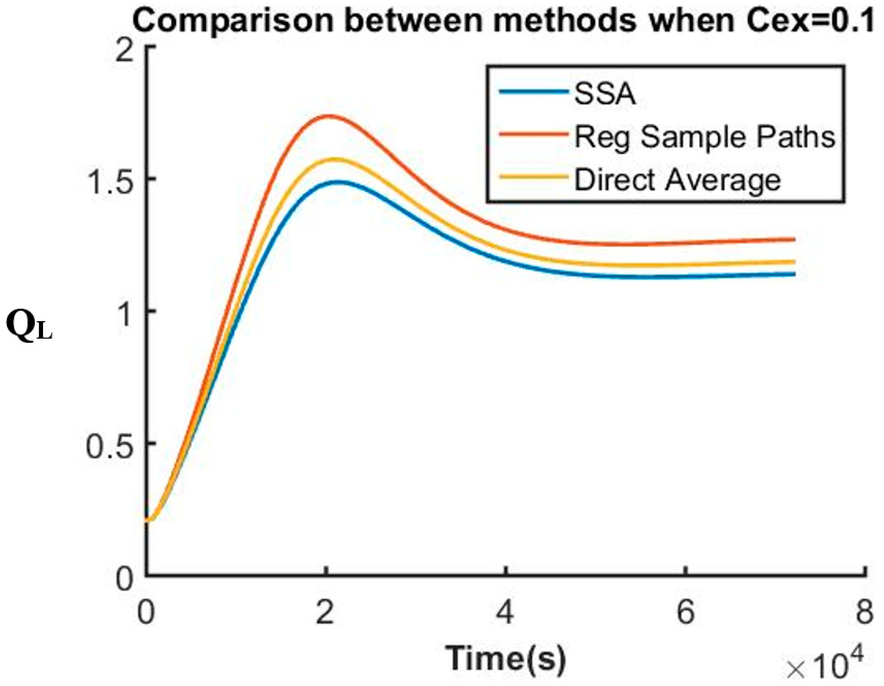
The system that is not only composed of a complex reaction network but also includes variables with stiff behaviors is indeed a good example to test the usefulness of this method. We simulate and compare the dynamics of key variables under different conditions using different methods by using SSA (Stochastic Simulation Algorithm) [1,2] as the benchmark. Results generated by utilizing the regular sample path method and the proposed direct-average method are presented together. Figure 1 below shows QL dynamics when the concentration of extracellular inducer is high.
In Figure 1, the three curves show similar expected results for QL response plotted against the concentration of inducer cCF10. At a low concentration of inducer in the environment, QL level stays low, indicating that the cells stay inactivated and are not ready for any conjugation process. It is significant that the direct averaging method here is closer to the SSA even with a substantially smaller number of sample paths than that employed in the regular sample path averaging method. The two curves associated with the SSA method and the regular sample path method are both generated by averaging results from 100,000 independent sample paths. On the other hand, to evaluate the direct average of variables at each following time step in the direct method, 100 sample points are generated to approximate both variance and covariance shown in both Equations (4) and (5). The argument to justify our sampling of only 100 points to approximate variance and covariance comes from the fact that the fluctuation associated with the sample points is very small. At any given time point, the calculation is done based on the previous average time point directly. Because of that, even though each variable can fluctuate, it cannot fluctuate too much away from the actual average value. Unlike this proposed method, in both SSA or the regular sample path methods, each trajectory is independent from one another. Calculation at each time point depends only on the previous point in that same trajectory. As time progresses, this fluctuation can accumulate and can potentially drift from the calculated values far away from its actual average value. This phenomenon explains why usage of SSA or the regular sample path method requires a high number of trajectories in order to obtain accurate results. This system is also known to be stiff, and so an investigation of a scenario where QL changes drastically is needed for a complete evaluation of this method. Figure 2 below represents QL response at a high concentration of inducer in the environment:
Figure 2 shows good agreement among results generated from all three methods. The same number of trajectories is utilized to compute the average in the SSA and the regular sample path methods. A high concentration of inducer immediately results in a stiff increase of QL, indicating a high sensitivity level of QL with respect to the inducer. In both cases shown in Figure 1 and Figure 2, the curves generated by the direct average method show less deviation from the “actual” solution (generated by the SSA method). The small deviation is a result of computing variable at each time point directly using the average values from the previous time point. The errors associated with the results generated by the regular sample path method and the direct average methods using SSA as the benchmark are 16% and 7% in the first case, and 11% and 6% in the second case, respectively. Figure 3 below shows the full-scale dynamic simulation for QL at various inducer levels in the environment.
This full range of calculations can serve to provide an overall picture of how the system would respond under different conditions. These results can also be used to provide inputs for experimentalists to develop the experimental design space in the most effective way. To complete the evaluation of the current method, simulation time is utilized for comparison among methods. The average step size of SSA method is selected to be a base unit from which the step sizes for other methods can be chosen. Time steps for the regular sample path and the direct average methods are both pre-selected to be ten-fold larger than the base unit. Figure 3 below provides a comparison in simulation times required by the three methods.
Figure 4 has on the ordinate the ratio between required simulation times for the direct method as well as the regular sample path method (i.e., using tau-leap) and the SSA. For various levels of cCF10, our direct method of generating sample paths for the mean and standard deviation of the stochastic process with Milstein’s method requires about two-fold less in CPU time as compared to that in the SSA. The parallelization strategy [10] developed by our group has also been implemented in obtaining results in the sample path methods using Milstein’s algorithm and SSA. The direct average method shows its advantage over the regular sample path strategy by reducing the simulation time by about half. Both methods become more effective as the concentration of cCF10 increases. The explanation for this comes from how the system or QL specifically in this case is sensitive with an increase of inducer in the environment. As the stiffness increases, the change in variables drastically increases, which in turn results in finer discretization steps for SSA, and hence increasing the simulation time for SSA.
5. Conclusions
Stochastic differential equations are widely used as approximate methods to obtain solutions for the master equation. The advantage of utilizing this type of equation is to smooth out solution behaviors (continuous responses) and to reduce the time steps in simulations. However, the explicit versions of SDE show little capability for capturing systems with stiff behaviors. Moreover, due to the unbounded features, it is also known that the methods can sometimes inaccurately predict results in some systems. Implicit SDE methods can describe stiff behaviors with a high efficacy but involve solving a large number of algebraic equations at each time point, resulting in a large increase in the CPU time. Recent work of Yin et al. [30] proposed an improved Milstein method for stiff systems. The method has the advantage of capturing solutions for systems with stiff behaviors. However, it still requires considerable time to obtain the average simulated results by generating independent sample paths. Moreover, from the experimental perspective, average dynamic behaviors of variables in a stochastic system are much more important and needed for cross-validations. The strategy of computing directly the average system behavior and its variance presented in this paper circumvents the need for a large number of time-consuming sample paths. The effectiveness of this method is demonstrated by testing on a large complex biological system. The results generated by the proposed methods show high accuracy with less simulation time as compared to both SSA and the regular sample path method. This strategy can also extend to other methods and can potentially offer an efficient way to obtain the average with a shorter CPU time. The development shown in this paper involved Taylor series expansion up to the second order term only. Testing this method on many other examples would help assess whether higher order terms in the Taylor expansion would be needed for increased accuracy level.
Supplementary Materials
The following are available online at https://www.mdpi.com/2227-9717/7/3/132/s1, Table S1: Reactions and kinetic parameters; Table S2: Degradation rates for different species.
Author Contributions
Conceptualization, D.R.; Methodology, V.T. and D.R.; Software, V.T.; Validation, V.T.; Formal Analysis, V.T. and D.R.; Writing—Original Draft Preparation, D.R.
Funding
This research was funded by National Institutes of Health Grant GM081888 (to Wei-Shou Hu).
Conflicts of Interest
The authors declare no conflict of interest.
References
- Shah, B.H.; Ramkrishna, D.; Borwanker, J.D. Simulation of particulate systems using the concept of the interval of quiescence. AIChE J. 1977, 23, 897–904. [Google Scholar] [CrossRef]
- Ramkrishna, D. Analysis of population balances-IV. The precise connection between Monte Carlo simulations and population balances. Chem.Eng.Sci. 1981, 36, 1203–1209. [Google Scholar] [CrossRef]
- Gillespie, D.T. Exact Stochastic Simulation of Coupled Chemical Reactions. J. Phys. Chem. 1977, 81, 2340–2361. [Google Scholar] [CrossRef]
- Gibson, M.A.; Bruck, J. Efficient Exact Stochastic Simulation of Chemical Systems with Many Species and Many Channels. J. Phys. Chem. A 2000, 104, 1876–1889. [Google Scholar] [CrossRef] [Green Version]
- Rathinam, M.; Petzold, L.R.; Cao, Y.; Gillespie, D.T. Consistency and Stability of Tau-Leaping Schemes for Chemical Reaction Systems. Multiscale Model. Simul. 2005, 4, 867–895. [Google Scholar] [CrossRef] [Green Version]
- Cao, Y.; Gillespie, D.T.; Petzold, L.R. Efficient step size selection for the tau-leaping simulation method. J. Chem. Phys. 2006, 124, 044109. [Google Scholar] [CrossRef] [PubMed]
- Tian, T.; Burrage, K. Binomial leap methods for simulating stochastic chemical kinetics. J. Chem. Phys. 2004, 121, 10356–10364. [Google Scholar] [CrossRef] [PubMed]
- Chatterjee, A.; Vlachos, D.G.; Katsoulakis, M.A. Binomial distribution based τ-leap accelerated stochastic simulation. J. Chem. Phys. 2005, 122, 024112. [Google Scholar] [CrossRef] [PubMed]
- Ramkrishna, D.; Shu, C.C.; Tran, V. New “Tau-Leap” strategy for stochastic simulation. Ind. Eng. Chem. Res. 2014, 53, 18975–18981. [Google Scholar] [CrossRef] [PubMed]
- Shu, C.C.; Tran, V.; Binagia, J.; Ramkrishna, D. On speeding up stochastic simulations by parallelization of random number generation. Chem. Eng. Sci. 2015, 137, 828–836. [Google Scholar] [CrossRef] [PubMed] [Green Version]
- Tran, V.; Ramkrishna, D. On facilitated computation of mesoscopic behavior of reaction-diffusion systems. AIChE J. 2017, 63, 5258–5266. [Google Scholar] [CrossRef]
- Grima, R. An effective rate equation approach to reaction kinetics in small volumes: Theory and application to biochemical reactions in nonequilibrium steady-state conditions. J. Chem. Phys. 2010, 133, 035101. [Google Scholar] [CrossRef] [PubMed]
- Gillespie, D.T. The multivariate Langevin and Fokker–Planck equations. Am. J. Phys. 1996, 64, 1246–1257. [Google Scholar] [CrossRef]
- Gillespie, D.T. The chemical Langevin equation. J. Chem. Phys. 2000, 113, 297–306. [Google Scholar] [CrossRef] [Green Version]
- Vilar, J.M.G.; Kueh, H.Y.; Barkai, N.; Leibler, S. Mechanisms of noise-resistance in genetic oscillators. Proc. Natl. Acad. Sci. USA 2002, 99, 5988–5992. [Google Scholar] [CrossRef] [PubMed] [Green Version]
- Wilkinson, D.J. Stochastic modelling for quantitative description of heterogeneous biological systems. Nat. Rev. Genet. 2009, 10, 122–133. [Google Scholar] [CrossRef] [PubMed]
- Turner, T.E.; Schnell, S.; Burrage, K. Stochastic approaches for modelling in vivo reactions. Comput. Biol. Chem. 2004, 28, 165–178. [Google Scholar] [CrossRef] [PubMed] [Green Version]
- Haseltine, E.L.; Rawlings, J.B. Approximate simulation of coupled fast and slow reactions for stochastic chemical kinetics. J. Chem. Phys. 2002, 117, 6959–6969. [Google Scholar] [CrossRef] [Green Version]
- Bruti-Liberati, N.; Platen, E. Strong approximations of stochastic differential equations with jumps. J. Comput. Appl. Math. 2007, 205, 982–1001. [Google Scholar] [CrossRef] [Green Version]
- Fiisiro-Maruyama, B. Continuous Markov Porcesses and Stochastic Equations; Springer: New York, NY, USA, 1955. [Google Scholar]
- Higham, D.J. An Algorithmic Introduction to Numerical Simulation of Stochastic Differential Equations. SIAM Rev. 2001, 43, 525–546. [Google Scholar] [CrossRef] [Green Version]
- Rüemelin, W. Numerical Treatment of Stochastic Differential Equations. SIAM J. Numer. Anal. 1982, 19, 604–613. [Google Scholar] [CrossRef]
- Rao, N.J.; Borwankar, J.D.; Ramkrishna, D. Numerical Solution of Ito Intergral Equations. SIAM J. Numer. Anal. 1974, 12, 124–139. [Google Scholar]
- Milstein, G.N.; Platen, E.; Schurz, H. Balance Implicit methods for Stiff Stochastic Systems. SIAM J. Numer. Anal. 1998, 35, 1010–1019. [Google Scholar] [CrossRef]
- Alcock, J.; Burrage, K. A note on the Balanced method. BIT Numer. Math. 2006, 46, 689–710. [Google Scholar] [CrossRef]
- Burrage, K.; Tian, T. The composite Euler method for stiff stochastic differential equations. J. Comput. Appl. Math. 2001, 131, 407–426. [Google Scholar] [CrossRef] [Green Version]
- Omar, M.A.; Aboul-Hassan, A.; Rabia, S.I. The composite Milstein methods for the numerical solution of Stratonovich stochastic differential equations. Appl. Math. Comput. 2009, 215, 727–745. [Google Scholar] [CrossRef]
- Wang, X.; Gan, S.; Wang, D. A family of fully implicit Milstein methods for stiff stochastic differential equations with multiplicative noise. BIT Numer. Math. 2012, 52, 741–772. [Google Scholar] [CrossRef]
- Tian, T.; Burrage, K. Implicit Taylor methods for stiff stochastic differential equations. Appl. Numer. Math. 2001, 38, 167–185. [Google Scholar] [CrossRef]
- Yin, Z.; Gan, S. An improved Milstein method for stiff stochastic differential equations. Adv. Differ. Equat. 2015, 2015, 369. [Google Scholar] [CrossRef]
- Gardiner, C.W. Stochastic Methods: A Handbook for the Natural and Social Sciences, 4th ed.; Springer: Berlin, Germany, 2009. [Google Scholar]
- Chatterjee, A.; Cook, L.C.C.; Shu, C.-C.; Chen, Y.; Manias, D.A.; Ramkrishna, D.; Dunny, G.M.; Hu, W.-S. Antagonistic self-sensing and mate-sensing signaling controls antibiotic-resistance transfer. Proc. Natl. Acad. Sci. USA 2013, 110, 7086–7090. [Google Scholar] [CrossRef] [PubMed] [Green Version]
- Tran, V. Davidson School of Chemical Engineering. Ph.D. Thesis, Purdue University, West Lafayette, IN, USA, 2018. [Google Scholar]
- Chatterjee, A.; Johnson, C.M.; Shu, C.C.; Kaznessis, Y.N.; Ramkrishna, D.; Hu, W.-S. Convergent transcription confers a bistable switch in Enterococcus faecalis conjugation. Proc. Natl. Acad. Sci. USA 2011, 108, 9721–9726. [Google Scholar] [CrossRef] [PubMed] [Green Version]
Figure 1.
QL dynamics at a low extracellular inducer concentration (SSA: Stochastic Simulation Algorithm).
Figure 1.
QL dynamics at a low extracellular inducer concentration (SSA: Stochastic Simulation Algorithm).

Figure 2.
QL level at a high level of inducer.

Figure 3.
QL response at various cCF10.

Figure 4.
Simulation time of the regular sample path method and direct averaging relative to that by SSA.
Figure 4.
Simulation time of the regular sample path method and direct averaging relative to that by SSA.

© 2019 by the authors. Licensee MDPI, Basel, Switzerland. This article is an open access article distributed under the terms and conditions of the Creative Commons Attribution (CC BY) license (http://creativecommons.org/licenses/by/4.0/).
Share and Cite
MDPI and ACS Style
Tran, V.; Ramkrishna, D. Simulating Stochastic Populations. Direct Averaging Methods. Processes 2019, 7, 132. https://doi.org/10.3390/pr7030132
AMA Style
Tran V, Ramkrishna D. Simulating Stochastic Populations. Direct Averaging Methods. Processes. 2019; 7(3):132. https://doi.org/10.3390/pr7030132
Chicago/Turabian StyleTran, Vu, and Doraiswami Ramkrishna. 2019. "Simulating Stochastic Populations. Direct Averaging Methods" Processes 7, no. 3: 132. https://doi.org/10.3390/pr7030132
Note that from the first issue of 2016, this journal uses article numbers instead of page numbers. See further details here.