Calibration of Discrete-Element-Method Parameters for Cohesive Materials Using Dynamic-Yield-Strength and Shear-Cell Experiments

Abstract
:1. Introduction and Objectives
- DEM simulations are computationally expensive and take a long time to complete due to small time-step sizes and large numbers of particles that are tracked as they move through the system.
- The approximation of complex particle shapes using spheres, usually done to reduce computational burden, might not reflect the true nature of the particles being simulated.
- Calibration of DEM parameters to match particle flow behavior in the experimental system is a challenge.
- Develop a DEM model for dynamic-yield-strength measurements and use it to calibrate the surface energy between particles.
- Develop a DEM model for a parallel-plate shear cell and calibrate the coefficient of sliding friction (CoSF) and the coefficient of rolling friction (CoRF) parameters for particle–particle interactions.
2. Experiment Setup
2.1. Materials
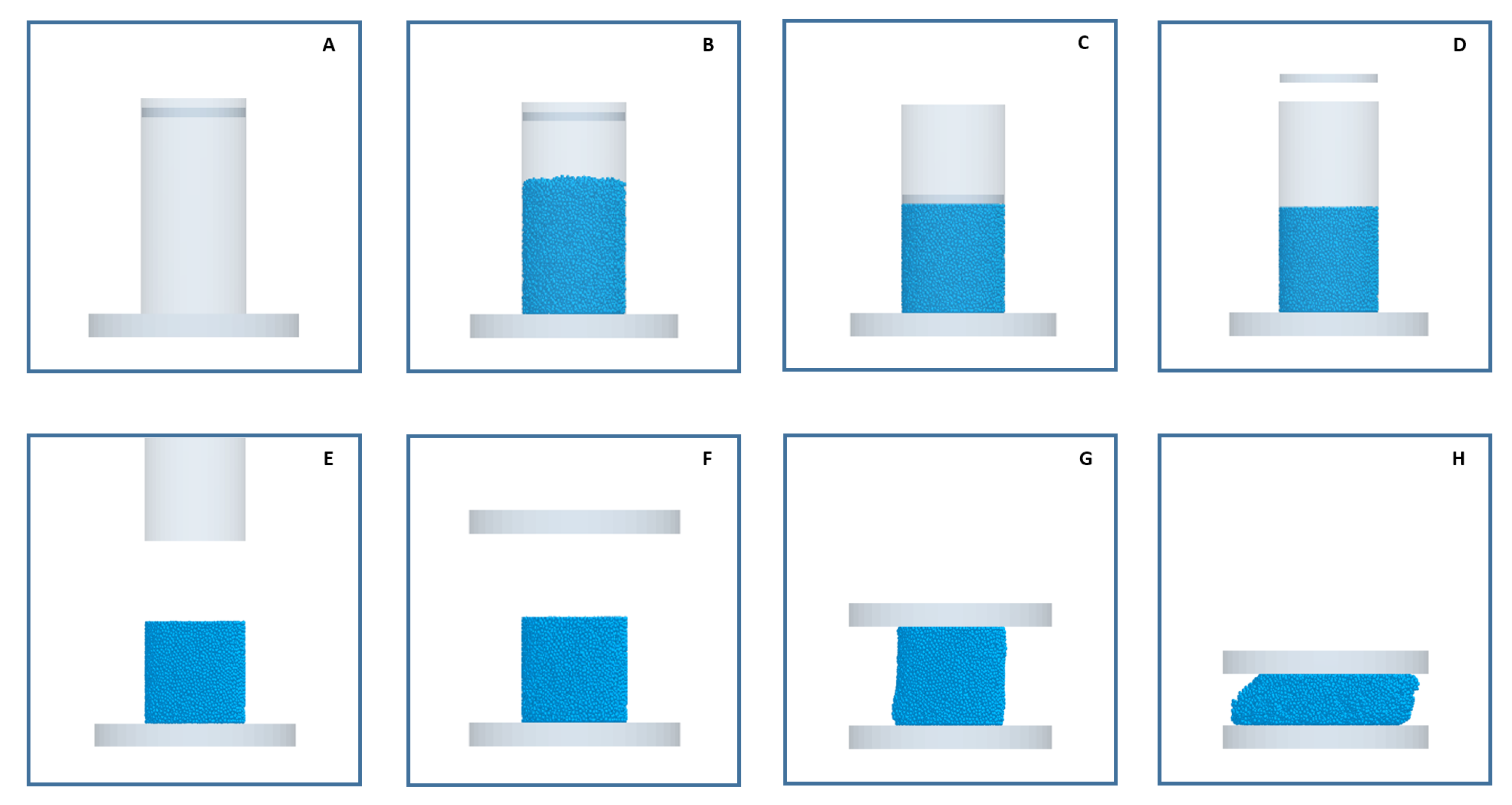
2.2. Dynamic Yield Strength Experiment
2.3. Shear-Cell Experiment
3. Method and Simulation Setups
3.1. Dynamic-Yield-Strength Simulation Setup
3.2. Periodic Shear-Cell Simulation Setup
4. Results and Discussion
4.1. Sensitivity Analysis: Dynamic Yield Strength
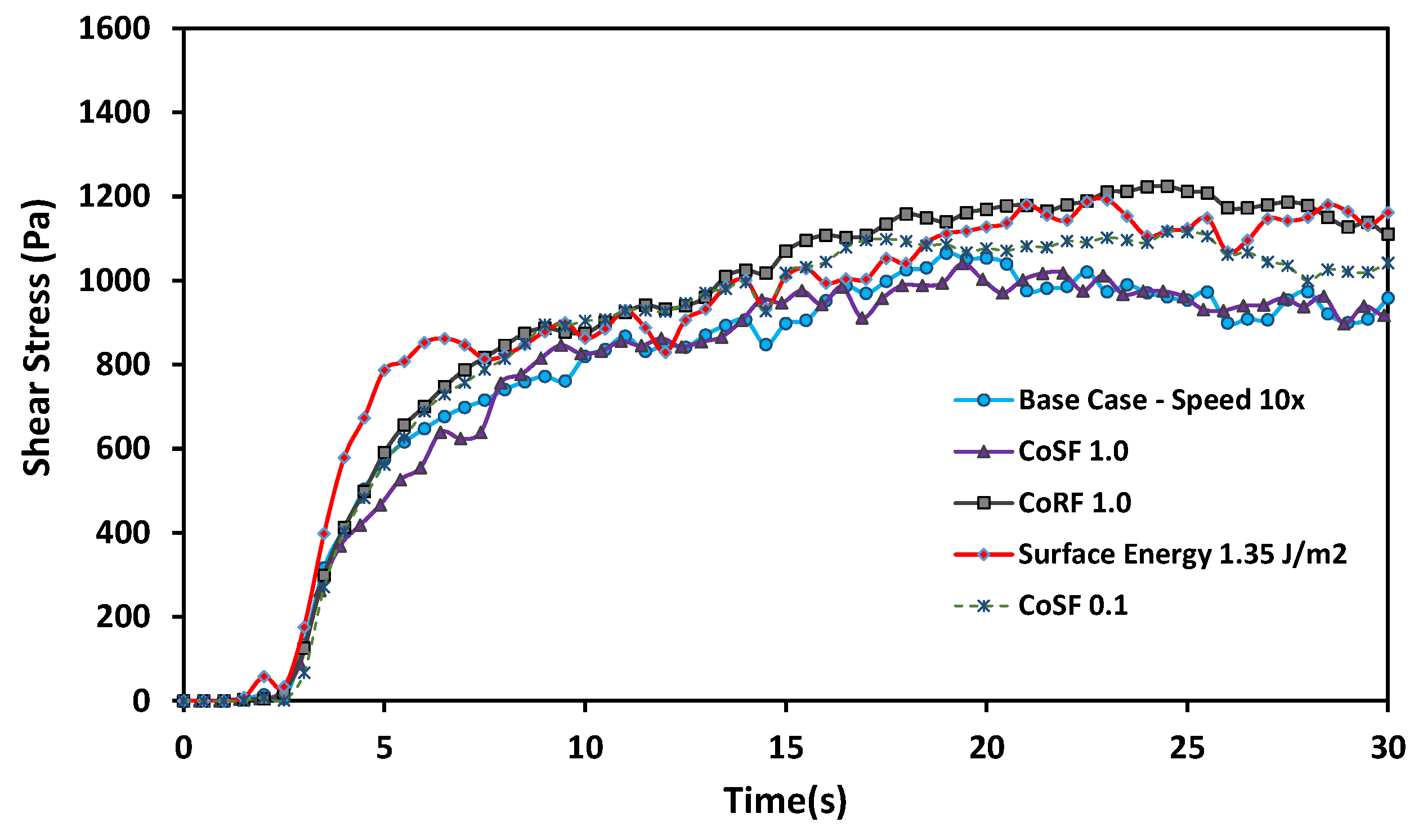
4.2. Shear-Cell Sensitivity Results
4.3. Surface-Energy Calibration Using DYS Simulations
- A different particle shear modulus chosen for the simulations. Here, a shear modulus of 1e7 Pa was tested.
- Particles were scaled-up for the simulations. Particle sizes were doubled for this test.
- Different sets of friction parameters were used. Both friction parameters were set to 0.5 for this test.
4.4. Comparing Calibrated Setups with Shear Cell
5. Conclusions
Author Contributions
Funding
Acknowledgments
Conflicts of Interest
Abbreviations
| CoRF | Coefficient of Rolling Friction |
| CoSF | Coefficient of Static Friction |
| DEM | Discrete Element Method |
| DYS | Dynamic Yield Strength |
References
- Hou, Q.; Dong, K.; Yu, A. DEM study of the flow of cohesive particles in a screw feeder. Powder Technol. 2014, 256, 529–539. [Google Scholar] [CrossRef]
- Li, H.; McCarthy, J.J. Controlling Cohesive Particle Mixing and Segregation. Phys. Rev. Lett. 2003, 90, 184301. [Google Scholar] [CrossRef] [PubMed]
- Thompson, M.; Sun, J. Wet granulation in a twin-screw extruder: Implications of screw design. J. Pharm. Sci. 2010, 99, 2090–2103. [Google Scholar] [CrossRef] [PubMed]
- Chen, Y.; Yang, J.; Dave, R.N.; Pfeffer, R. Granulation of cohesive Geldart group C powders in a Mini-Glatt fluidized bed by pre-coating with nanoparticles. Powder Technol. 2009, 191, 206–217. [Google Scholar] [CrossRef]
- Peron, H.; Delenne, J.; Laloui, L.; Youssoufi, M.E. Discrete element modelling of drying shrinkage and cracking of soils. Comput. Geotech. 2009, 36, 61–69. [Google Scholar] [CrossRef]
- Yu, S.; Gururajan, B.; Reynolds, G.; Roberts, R.; Adams, M.J.; Wu, C.Y. A comparative study of roll compaction of free-flowing and cohesive pharmaceutical powders. Int. J. Pharm. 2012, 428, 39–47. [Google Scholar] [CrossRef]
- Guaita, M.; Couto, A.; Ayuga, F. Numerical Simulation of Wall Pressure during Discharge of Granular Material from Cylindrical Silos with Eccentric Hoppers. Biosyst. Eng. 2003, 85, 101–109. [Google Scholar] [CrossRef]
- Prescott, J.; Bernum, R. On Powder Flowability. Pharm. Technol. 2000, 24, 60–84. [Google Scholar]
- Cundall, P.A.; Strack, O.D.L. A discrete numerical model for granular assemblies. Géotechnique 1979, 29, 47–65. [Google Scholar] [CrossRef]
- Ketterhagen, W.R.; am Ende, M.T.; Hancock, B.C. Process Modeling in the Pharmaceutical Industry using the Discrete Element Method. J. Pharm. Sci. 2009, 98, 442–470. [Google Scholar] [CrossRef]
- Mitarai, N.; Nori, F. Wet granular materials. Adv. Phys. 2006, 55, 1–45. [Google Scholar] [CrossRef] [Green Version]
- Johnson, K.L.; Kendall, K.; Roberts, A.D. Surface Energy and the Contact of Elastic Solids. Proc. R. Soc. Lond. Ser. A Math. Phys. Sci. 1971, 324, 301–313. [Google Scholar] [CrossRef]
- Lian, G.; Thornton, C.; Adams, M.J. A Theoretical Study of the Liquid Bridge Forces between Two Rigid Spherical Bodies. J. Colloid Interface Sci. 1993, 161, 138–147. [Google Scholar] [CrossRef]
- Mikami, T.; Kamiya, H.; Horio, M. Numerical simulation of cohesive powder behavior in a fluidized bed. Chem. Eng. Sci. 1998, 53, 1927–1940. [Google Scholar] [CrossRef]
- Umer, M.; Siraj, M.S. DEM studies of polydisperse wet granular flows. Powder Technol. 2018, 328, 309–317. [Google Scholar] [CrossRef]
- Mukherjee, R.; Mao, C.; Chattoraj, S.; Chaudhuri, B. DEM based computational model to predict moisture induced cohesion in pharmaceutical powders. Int. J. Pharm. 2018, 536, 301–309. [Google Scholar] [CrossRef]
- Guo, Y.; Wassgren, C.; Ketterhagen, W.; Hancock, B.; Curtis, J. Discrete element simulation studies of angles of repose and shear flow of wet, flexible fibers. Soft Matter 2018, 14, 2923–2937. [Google Scholar] [CrossRef]
- Radl, S.; Kalvoda, E.; Glasser, B.J.; Khinast, J.G. Mixing characteristics of wet granular matter in a bladed mixer. Powder Technol. 2010, 200, 171–189. [Google Scholar] [CrossRef]
- Wu, W.; Tu, Z.; Zhu, Z.; Zhang, Z.; Lin, Y. Effect of Gradation Segregation on Mechanical Properties of an Asphalt Mixture. Appl. Sci. 2019, 9. [Google Scholar] [CrossRef]
- Brenda, R.; Khinast, J.G.; Glasser, B.J. Wet granular flows in a bladed mixer: Experiments and simulations of monodisperse spheres. AIChE J. 2012, 58, 3354–3369. [Google Scholar]
- Marigo, M.; Stitt, E.H. Discrete Element Method (DEM) for Industrial Applications: Comments on Calibration and Validation for the Modelling of Cylindrical Pellets. KONA Powder Part. J. 2015, 32, 236–252. [Google Scholar] [CrossRef]
- Li, Y.; Xu, Y.; Thornton, C. A comparison of discrete element simulations and experiments for ‘sandpiles’ composed of spherical particles. Powder Technol. 2005, 160, 219–228. [Google Scholar] [CrossRef]
- Sen, M.; Karkala, S.; Panikar, S.; Lyngberg, O.; Johnson, M.; Marchut, A.; Schäfer, E.; Ramachandran, R. Analyzing the Mixing Dynamics of an Industrial Batch Bin Blender via Discrete Element Modeling Method. Processes 2017, 5. [Google Scholar] [CrossRef]
- Zhou, Y.; Xu, B.; Yu, A.; Zulli, P. An experimental and numerical study of the angle of repose of coarse spheres. Powder Technol. 2002, 125, 45–54. [Google Scholar] [CrossRef]
- Do, H.Q.; Aragón, A.M.; Schott, D.L. Automated discrete element method calibration using genetic and optimization algorithms. EPJ Web Conf. 2017, 140, 15011. [Google Scholar] [CrossRef] [Green Version]
- Simons, T.A.; Weiler, R.; Strege, S.; Bensmann, S.; Schilling, M.; Kwade, A. A Ring Shear Tester as Calibration Experiment for DEM Simulations in Agitated Mixers—A Sensitivity Study. Procedia Eng. 2015, 102, 741–748. [Google Scholar] [CrossRef]
- Cheng, H.; Shuku, T.; Thoeni, K.; Tempone, P.; Luding, S.; Magnanimo, V. An iterative Bayesian filtering framework for fast and automated calibration of DEM models. Comput. Methods Appl. Mech. Eng. 2019, 350, 268–294. [Google Scholar] [CrossRef]
- Ostanin, I.; Wang, Y.; Ni, Y.; Dumitrică, T. Mechanics of Nanocrystalline Particles With the Distinct Element Method. J. Eng. Mater. Technol. 2015, 137, 024501. [Google Scholar] [CrossRef]
- Asaf, Z.; Rubinstein, D.; Shmulevich, I. Determination of discrete element model parameters required for soil tillage. Soil Tillage Res. 2007, 92, 227–242. [Google Scholar] [CrossRef]
- Tsunazawa, Y.; Fujihashi, D.; Fukui, S.; Sakai, M.; Tokoro, C. Contact force model including the liquid-bridge force for wet-particle simulation using the discrete element method. Adv. Powder Technol. 2016, 27, 652–660. [Google Scholar] [CrossRef]
- Wang, Y.; Xu, H.; Drozdov, G.; Dumitrică, T. Mesoscopic friction and network morphology control the mechanics and processing of carbon nanotube yarns. Carbon 2018, 139, 94–104. [Google Scholar] [CrossRef]
- Hare, C.; Zafar, U.; Ghadiri, M.; Freeman, T.; Clayton, J.; Murtagh, M. Analysis of the dynamics of the FT4 powder rheometer. Powder Technol. 2015, 285, 123–127. [Google Scholar] [CrossRef] [Green Version]
- Zafar, U.; Hare, C.; Hassanpour, A.; Ghadiri, M. Drop test: A new method to measure the particle adhesion force. Powder Technol. 2014, 264, 236–241. [Google Scholar] [CrossRef] [Green Version]
- DEM Solutions. EDEM 2.5.1 Documentation. EDEM Analyst. 2013. Available online: http://www.dem--solutions.com/ (accessed on 29 April 2019).
- Dassault Systémes. Solidworks 2010–2011 Documentation. Solidworks Fundamentals. 2010. Available online: http://www.solidworks.com/ (accessed on 29 April 2019).
- Nasato, D.S.; Goniva, C.; Pirker, S.; Kloss, C. Coarse Graining for Large-scale DEM Simulations of Particle Flow—An Investigation on Contact and Cohesion Models. Procedia Eng. 2015, 102, 1484–1490. [Google Scholar] [CrossRef]
- Baran, O.; DeGennaro, A.; Ramé, E.; Wilkinson, A. DEM Simulation of a Schulze Ring Shear Tester. AIP Conf. Proc. 2009, 1145, 409–412. [Google Scholar]
- Mindlin, R.; Deresiewicz, H. Elastic Spheres in Contact under Varying Oblique Force. J. Appl. Mech. 1953, 20, 327–344. [Google Scholar]
- Liu, J.; Yun, B.; Zhao, C. Identification and Validation of Rolling Friction Models by Dynamic Simulation of Sandpile Formation. Int. J. Geomech. 2012, 12, 484–493. [Google Scholar] [CrossRef]
- Ting, J.M.; Khwaja, M.; Meachum, L.R.; Rowell, J.D. An ellipse-based discrete element model for granular materials. Int. J. Numer. Anal. Methods Geomech. 1993, 17, 603–623. [Google Scholar] [CrossRef]
- Ketterhagen, W.R.; Curtis, J.S.; Wassgren, C.R.; Hancock, B.C. Predicting the flow mode from hoppers using the discrete element method. Powder Technol. 2009, 195, 1–10. [Google Scholar] [CrossRef]


| Properties | Blend |
|---|---|
| Bulk Density () | 422 |
| D50 () | 14.30 |
| Avg. Flow Factor | 1.7 |
| Material Parameters | Particle | Wall |
|---|---|---|
| Density () | 1000 | 8000 |
| Poisson’s Ratio | 0.2 | 0.33 |
| Shear Modulus (Pa) | ||
| Surface Energy () | 0.45 | - |
| Interaction Parameters | Particle-Particle | Particle-Wall |
|---|---|---|
| Coeff. of Restitution | 0.2 | 0.2 |
| Coeff. of Sliding Friction | 0.4 | 0 |
| Coeff. of Rolling Friction | 0.01 | 0 |
| Simulation | Parameter Value | DYS (Pa) | Change w.r.t. Base Case (%) |
|---|---|---|---|
| Base case | - | 495 | - |
| Poisson’s Ratio | 0.5 | 457 | −7.7 |
| Coeff. of Restitution | 0.5 | 472 | −4.6 |
| Shear Modulus (Pa) | 400 | −19.2 | |
| Surface Energy () | 1.125 | 1853 | 274.3 |
| Coeff. of Sliding Friction | 1.0 | 402 | −18.8 |
| Coeff. of Rolling Friction | 0.025 | 678 | 37.0 |
| Simulation | Surface Energy () | DYS (Pa) |
|---|---|---|
| Target/Experimental result | - | 3242 |
| Calibrated base case (CBC) | 2.15 | 3378 |
| Shear modulus Pa | 2.95 | 3220 |
| Double particle size | 2.90 | 3351 |
| CoSF and CoRF 0.5 | 0.95 | 3267 |
© 2019 by the authors. Licensee MDPI, Basel, Switzerland. This article is an open access article distributed under the terms and conditions of the Creative Commons Attribution (CC BY) license (http://creativecommons.org/licenses/by/4.0/).
Share and Cite
Karkala, S.; Davis, N.; Wassgren, C.; Shi, Y.; Liu, X.; Riemann, C.; Yacobian, G.; Ramachandran, R. Calibration of Discrete-Element-Method Parameters for Cohesive Materials Using Dynamic-Yield-Strength and Shear-Cell Experiments. Processes 2019, 7, 278. https://doi.org/10.3390/pr7050278
Karkala S, Davis N, Wassgren C, Shi Y, Liu X, Riemann C, Yacobian G, Ramachandran R. Calibration of Discrete-Element-Method Parameters for Cohesive Materials Using Dynamic-Yield-Strength and Shear-Cell Experiments. Processes. 2019; 7(5):278. https://doi.org/10.3390/pr7050278
Chicago/Turabian StyleKarkala, Subhodh, Nathan Davis, Carl Wassgren, Yanxiang Shi, Xue Liu, Christian Riemann, Gary Yacobian, and Rohit Ramachandran. 2019. "Calibration of Discrete-Element-Method Parameters for Cohesive Materials Using Dynamic-Yield-Strength and Shear-Cell Experiments" Processes 7, no. 5: 278. https://doi.org/10.3390/pr7050278
APA StyleKarkala, S., Davis, N., Wassgren, C., Shi, Y., Liu, X., Riemann, C., Yacobian, G., & Ramachandran, R. (2019). Calibration of Discrete-Element-Method Parameters for Cohesive Materials Using Dynamic-Yield-Strength and Shear-Cell Experiments. Processes, 7(5), 278. https://doi.org/10.3390/pr7050278