1. Introduction
The global energy crisis has become an urgent issue in the 21st century [
1]. The worldwide growth in energy consumption and carbon emissions is about 1.5% and 1.4% annually over the past 5 years [
2]. However, as the main form of energy, the remaining oil is forecasted to be available for only about 50 years [
2]. Furthermore, the oil refineries face various challenges: growing demand for high-quality and low-boiling point products, deterioration of crude oil, ever-increasing difficulty of petroleum processing, and stringent environmental requirements. Since vacuum residue accounts for about half of the crude oil, more attention has been focused on vacuum residue hydroconversion processes, which are capable of converting heavy, inferior petroleum into light, valuable products such as gasoline, jet fuel, and diesel [
3,
4]. A good process model is important for monitoring the plant-level operation status, optimizing operating conditions, verifying the dynamic adjustment scheme, and maximizing the profit [
5,
6,
7].
The residue hydrotreating process mainly consists of a reactor and a fractionation unit. The core of the process model is the kinetic model, which describes the catalytic cracking reactions based on mechanism knowledge. For the kinetic model, the inputs are the feedstock properties and reaction conditions. The model outputs are product yield, product properties, reactor temperature rise, and hydrogen consumption at different operation conditions. In the past years, two main kinds of methods have been studied to establish the kinetic model, which are based on molecular composition and lumped composition, respectively.
Based on molecular composition for the kinetic model, structure-oriented lumping (SOL) proposed by Quann et al. [
8] is one of the most widely used techniques. In this technique, the feedstock mixture was expressed as a matrix, whose rows indicated different atomic elements like C, H, S, N, O, and columns represented different structural groups. This technique was then applied to model the fluid catalytic cracking (FCC) of the naphtha hydrodesulfurization [
9]. Additionally, a two-step reconstruction algorithm was proposed by Hudebine et al. [
10]. This algorithm could rebuild petroleum at a molecular level from overall petroleum analyses. Moreover, Peng et al. [
11] investigated another approach called as the molecular type homologous series (MTHS), in which homologous series, along with carbon number information were considered for kinetic modeling. This approach obtained excellent predictions for a coal tar hydrogenation process [
12]. However, these methods are with a shortcoming of the computation expensiveness since extensive molecular compositions are generated in the kinetic model. Additionally, another shortcoming is that routine chemical analysis and
13C nuclear magnetic resonance (NMR) are required. However, these analyses are mostly performed with low frequency, which limits these molecular-level methods on applying in residue hydroconversion process simulations.
The lumped method, proposed by Weekman et al. [
13], was originally utilized for a three lumped model of a catalytic cracking process. In this method, the mixture of hydrocarbons was characterized by several lumped compositions classified by their reaction characteristics, which can alleviate the difficulty of building the complicated kinetic model. Then, the kinetic model is further extended to four [
14], five [
15], seven [
16], and even thirty-seven lumped models [
17]. However, those models only reflect the productivity, whereas some detailed information, such as sulfur and nitrogen content, is not included. Besides, once the lumps of kinetic model are determined, the cutting scopes of gasoline and distillate oil are permanent. However, the cutting scopes generally vary from refinery to refinery with different optimal economic benefits, which results in poor adaptability of the simulation models.
Hence, it is necessary to construct a reasonable model based on proper material compositions. The compositions should contain theoretical, circumstantial information sufficient to reflect the process. Meanwhile, proper number of compositions are required to easily make the calculation and give good extrapolation results. Fortunately, another approach is utilized in the Aspen HYSYS/Refining hydrocracker model to simulate the reaction process at the molecular level, in which 97 lumps are selected to characterize petroleum. Also, these lumps take both the carbon number and molecular structure information into consideration, which are in accordance with the results in the reported literatures [
18,
19]. These lumps can be grouped into three classes of paraffin (P), naphthene (N), and aromatics (A). They can be tested using mass spectrometry and adopted to describe light petroleum (i.e., the PNA method). However, the heavy vacuum residue is usually characterized by the method four components of saturate, aromatic, resin, and asphaltene (SARA). The PNA characterization method is different from SARA, which may be improper for simulating the vacuum residue hydrogenation process. In addition, high-boiling point resin and asphaltene are not represented by the lumps in the hydrocracker [
20,
21], which results in the lower high-boiling points of simulated petroleum. Moreover, the colloidal structure of resin, and asphaltene (RA) have a great impact on the overall kinetics [
22].
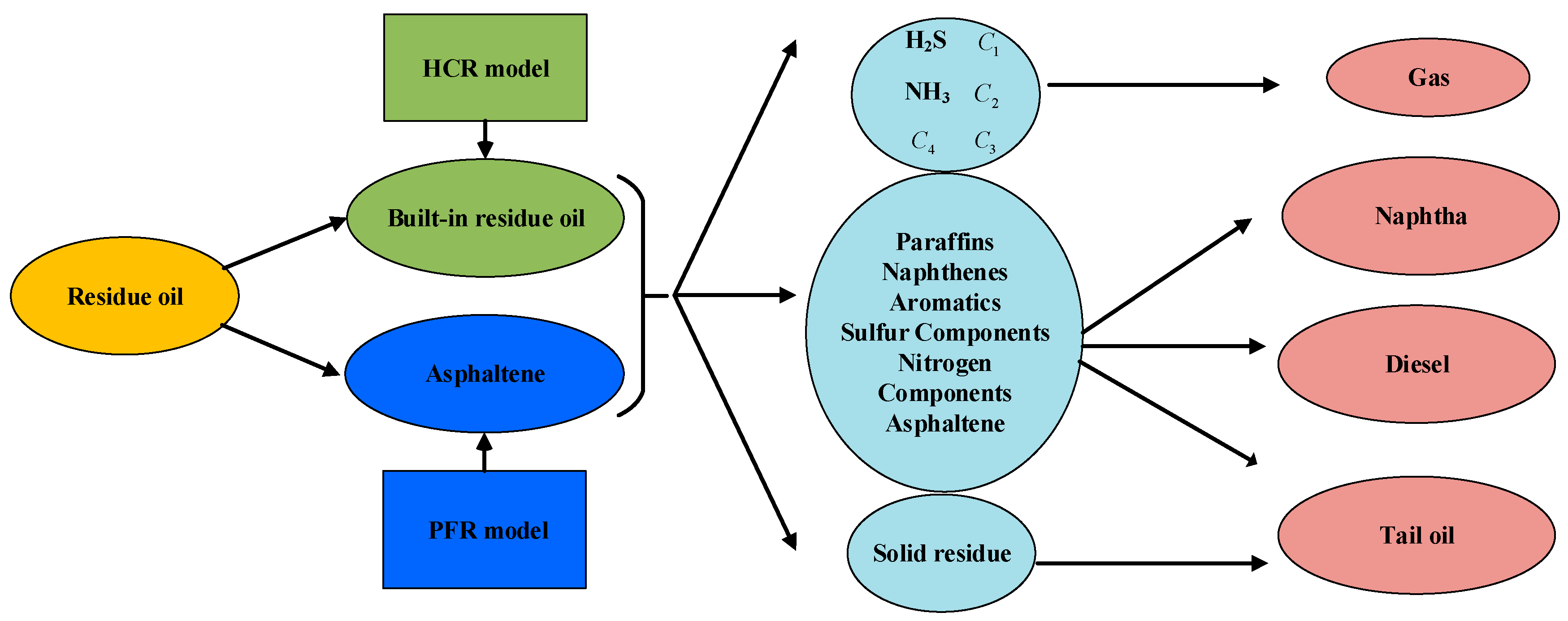
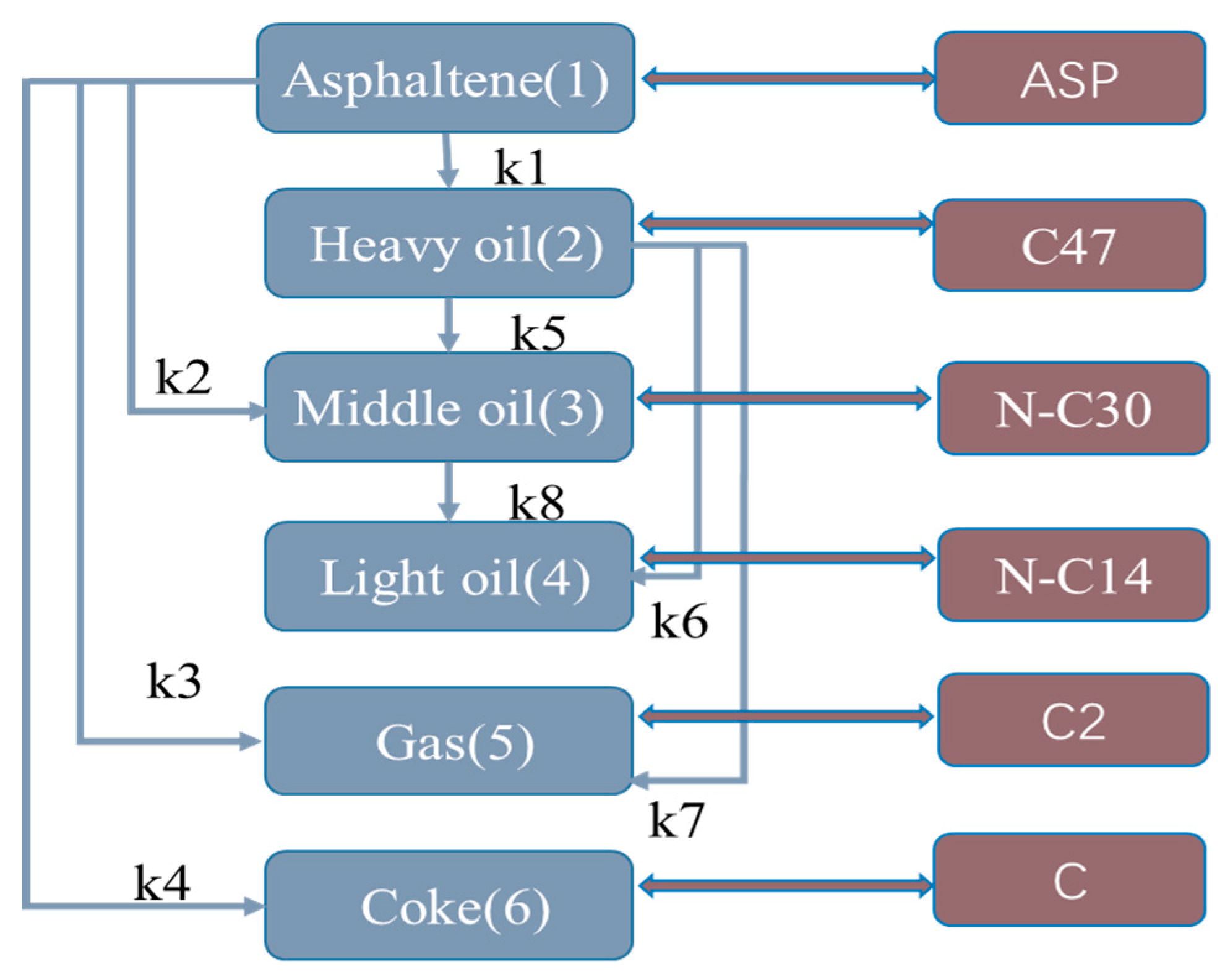
To alleviate the aforementioned problems, two parallel structure reactors model is proposed in this paper to simulate a real industrial residue hydrogenation process. The conversion process of the heavier petroleum regarded as an asphaltene lump is modeled in a plug flow reactor (PFR), which is in parallel with the original hydrocracker reactor (HCR) existing in Aspen HYSYS/Refining. In the PFR, the asphaltene conversion reaction network is established and its lumps are necessary to be characterized. To describe the asphaltene conversion, a six-lump reaction model is adopted. For the lump characterization, the property of asphaltene is calculated using the group contribution method, and the remaining lumps in the reaction model are represented utilizing the substitute mixtures of real components (SMRCs) method [
23]. And the HCR simulates lighter petroleum hydrogenation based on the built-in reaction network and lumps.
As the outermost layer of residue hydrogenation model, the process model seeks to integrate the reactor model with the fractionation model. Due to the complexity of residues, most previous works paid attention to only one aspect of the reactor model or the fractionator model for the for the plant wide residue hydrogenation process [
24]. To make contribution to this aspect, a residue hydroconversion process model is comprehensively developed by exploiting delumping, which is a committed step to concatenate the reactor with the fractionation model.
The paper is structured as follows:
Section 2 describes the residue hydrogenation process in detail.
Section 3 illustrates the kinetic model describing the hydrogenation process of built-in residue oil simulated in an HCR and asphaltene simulated in a PFR.
Section 4 demonstrates the framework for building the whole process model, which includes characterization of the feedstock mixture, establishment of a reactor model of two parallel structure reactors, and delumping of the reactor model effluent.
Section 5 presents the simulation results to clarify the model effectiveness.
Section 6 provides the conclusion.
2. Process Description
The residue hydrogenation technology is one of the most effective ways to deeply hydro treat the heavy oil. The process is implemented in fixed beds for removal of the majority of impurities from oils, which can supply excellent raw materials to the subsequent catalytic cracking process. In the fixed bed reactors, both hydrotreating and hydrocracking reactions take place in appropriate temperature, pressure, hydrogen–oil ratio, and liquid hourly space velocity (LHSV) conditions. Generally, four reactors are adopted and connected in series, and the main function of each reactor is to remove some specific impurities.
A schematic diagram of the residue hydrogenation unit is displayed in
Figure 1. The raw materials are blended with vacuum heavy wax oil, coke gas oil, tar wax oil and catalytic circulating oil. Before entering the reaction system, the blended oil is filtered in a buffer tank. Then the oil is boosted in the pump and exchanged heat with the reactor effluent. Afterwards, the oil goes through the heating furnace before entering the first reactor. Thus, the first reactor temperature is mainly affected by the heating furnace.
The temperatures of the rest ones are controlled by hydrogen quenching to attain the required operation conditions. In the hydrotreater (HT), sulfur, nitrogen, and oxygen compounds are mostly converted to hydrogen sulfide, ammonia, and water, while polycyclic aromatic hydrocarbons and some unsaturated hydrocarbons are hydro saturated.
The outflow from the last HT is then transferred to a high and low pressure separation system (HLPS) in which three-phase separation of the gas, oil and water takes place. The HLPS mainly consists of four separators, as illustrated in
Figure 1. The gas of the separators then enters a desulfurization tower to desorb hydrogen sulfide. After this operation, the hydrogen purity of recycled gas is improved. Meanwhile, the off-gas discharges a part of the
. The hydrogen is then compressed and blended with fresh hydrogen (
).The blended gas recycles back to the four reactors, in which a part of the recycled gas (RG) is mixed with feed oil, and the other gas functioned as gas quenching (
) quenches the beds to ensure security and protect the catalyst. And the bottom stream of the HLPS is delivered to the downstream: the fractionation process, which includes a fractionator, a diesel stripper, a condenser, and a pump. The top product of the fractionator is naphtha, the middle one is diesel, and the bottom one is tail oil.
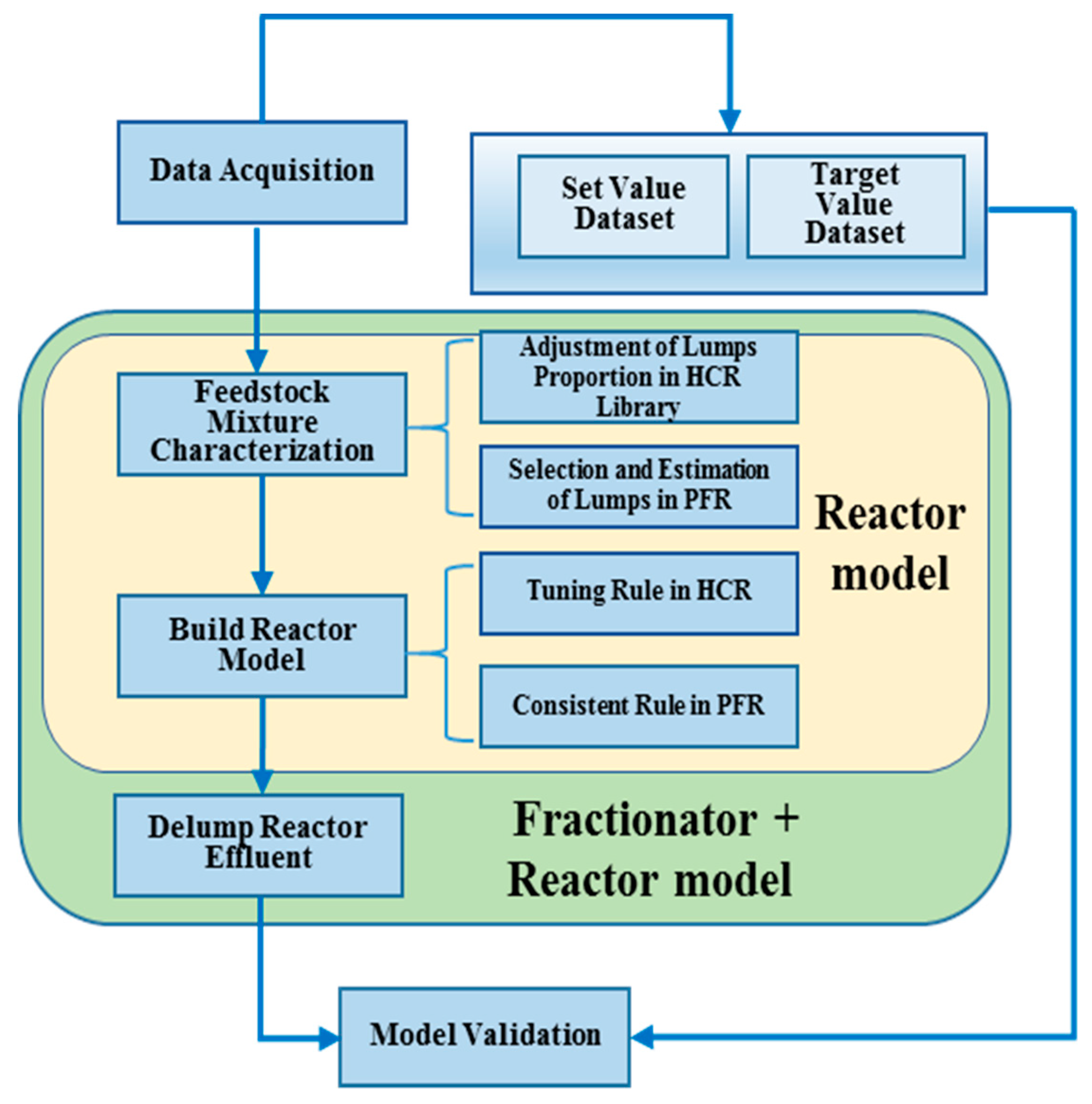
4. Workflow of Developing an Integrated Residue Hydrogenation Process Model
The workflow for developing an integrated residue hydrogenation model is shown in
Figure 5 with the Aspen HYSYS/Refining simulation software. A similar workflow for the hydrocracking process was proposed in [
24]. However, it is different for the heavy petroleum refining process.
First of all, residue tends to become inferior and heavier since the crude oil gets heavier. However, the feed library for residue is predetermined in the simulation software. Furthermore, the asphaltene with higher boiling point is not considered in the feed library. In addition, owing to the absence of asphaltene, its product lumps are lacking in the feed library. Thus, it is required to make some adjustments for the feed in the HCR library and characterize the added six lumps. Moreover, due to the different feed properties and reaction conditions, it is necessary to determine the kinetic parameters of the reactor model. In the HCR model, the reaction activity variables are to be estimated for the built-in residue oil hydrogenation. Correspondingly, in the PFR model, the kinetic parameters are determined for the additional asphaltene hydrogenation. Finally, the reactor model is established with kinetic lumps grouped by reaction characteristics, whereas the fractionation model is built based on the pseudo-components according to fractionation characteristic (i.e., the boiling point). Therefore, the adopted kinetic lumps of reactor model may be inappropriate for a fractionator modeling of residue hydrogenation process. Consequently, it is prerequisite to transform kinetic lumps into suitable pseudo-components through a process called delumping. The detailed workflow of the residue hydrogenation model can be described as follows:
- (1)
Obtain data from factories and select the required data for modeling. In this work, the set data (e.g., the feed property, flow) is the input of the model and the target data (e.g., the product yield, property) are the object value to be attained.
- (2)
Characterize the feedstock based on laboratory testing data.
- (3)
Develop the reactor model according to the real process data.
- (4)
Delump the effluent from the reactor to build the fractionator.
- (5)
Test the effectiveness of the model by comparing the model results with actual plant data.
4.1. Feedstock Mixture Characterization
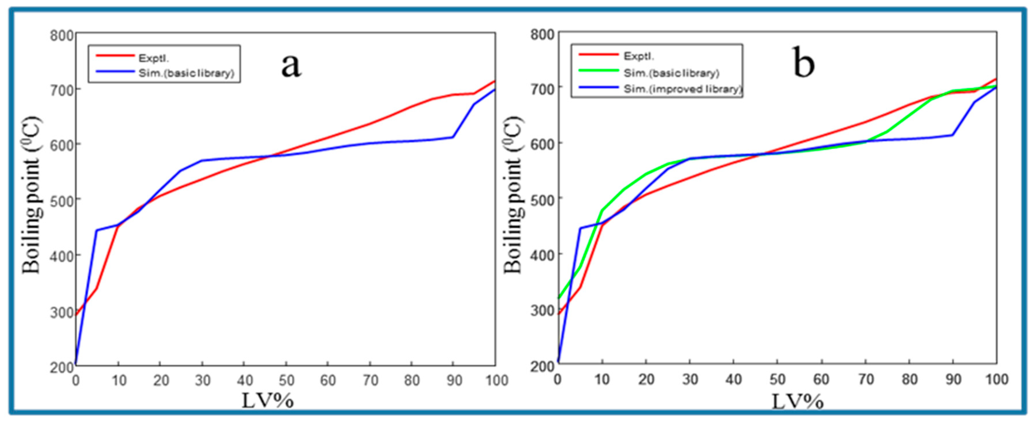
Feed quality has a significant influence on residue hydrogenation process. Thus, it is fundamental to characterize the feedstock mixture according to its bulk properties. In this work, the “residue” fingerprint type is selected in the basic feed library of HCR for the residue hydrogenation process. And the feed data section inputs are the experimental bulk properties of feed, such as its density, boiling point, refractive index, sulfur content, and nitrogen content. The corresponding outputs are the simulated bulk properties and composition contents. Generally, the experimental bulk properties diverge from the simulated.
Figure 6a show the residue properties of a dataset in the HCR. It can be found that the simulated initial boiling point (IBP) and final boiling point (FBP) are lower than their experimental values. Meanwhile, the simulated total light oil percentage is slightly higher in
Table 1, which may have impact on the simulated reactor performance. It is because that the conversion of actual weight residue hydrogenation is only 15–20%, which is defined as the sum of the weight proportions of gas and light oil after reaction. Therefore, two problems demand to be solved.
The first problem is that the lumped compositions whose normal boiling point is lower the real IBP value should be removed. Therefore, their proportion should be set to zero, which is based on the separation efficiency factor proposed by García et al. [
29]. In this way, the proportions of remaining lumps inevitably increase. To handle this problem, it is necessary to adjust the proportions, which has been presented in the previous work [
30].
Figure 6b and
Table 1 show the results of the experimental value, simulated value with basic and improved library of the residue feed. Since the distillation range of naphtha is lower than that of residue, the contribution of naphtha is 0% in
Table 1.
The other problem is that the simulated FBP of the feed is lower than its experimental value. Therefore, it is indispensable to add the composition representing the higher boiling point petroleum lump, and other lumps in the reaction network, which is displayed in
Figure 4. To represent the added petroleum, the composition of Tahe residue heavy resin is adopted from [
31], since its properties are closer to the real petroleum cut. Its properties of molecular weight and density are also given in reference [
31]. Although the software has a powerful ability to calculate physical property, at least three properties are required to characterize the lumps more precisely. Fortunately, the normal boiling point of petroleum cut can be estimated using the group contribution method [
32]. In this method, the composition (considered as a molecule here) is composed of 77 structural groups. Each group has its own contribution and can be referred to in reference [
33]. The molecule property is calculated by summing the products over each group numbers and its corresponding contribution. Meanwhile, the method of first-order group contributions is applied to predict the normal boiling point, which is shown in the following equation [
34]:
where
represents the group contribution of group
;
represents the number of group
in the molecule;
represents a regulatable parameter (
), and
represents a boiling point corrector, which can be computed as follows:
where
represents the number of rings in a molecule.
According to Equations (11) and (12), the normal boiling point of asphaltene is estimated, and other properties are calculated by the software. The results are shown in
Table 2.
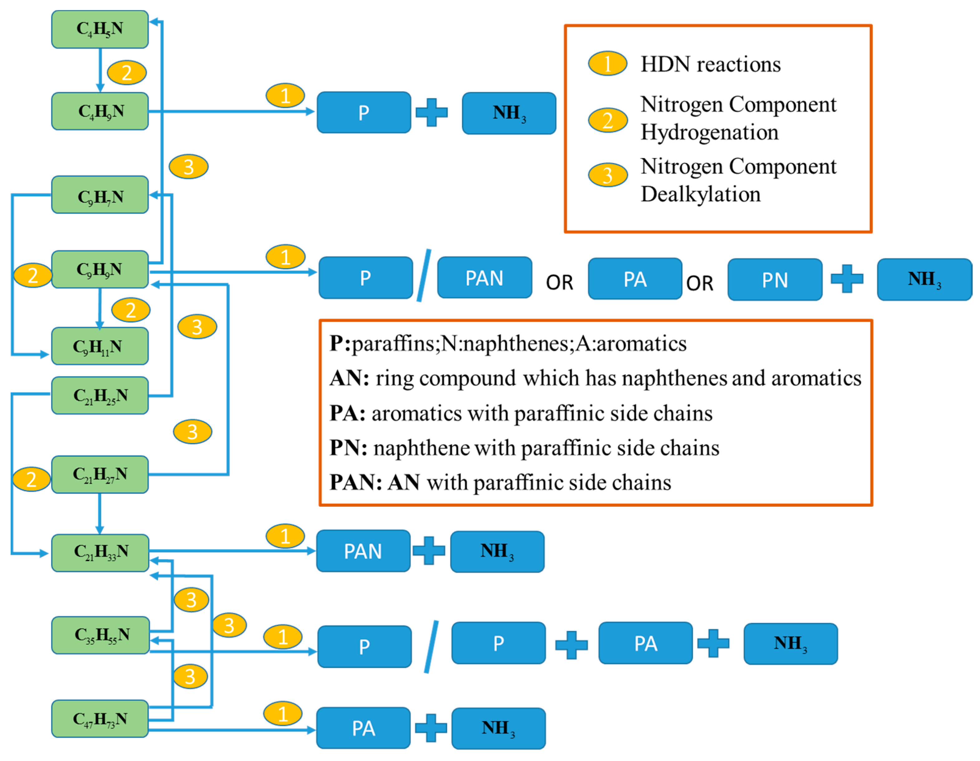
Then, the remaining five lumps need to be characterized in the reaction network. Here, the method of substitute mixtures of real components (SMRCs) is used for lump characterization. This method enhances comprehension of the mechanism of the reaction since the structure of a substituted component is included. In this method, each lump is substituted by one component whose normal boiling point approximates the average distillation range of the lump. Since multiple components may be available for a specified boiling point, it is important to select the proper components. The main principles are as follows: (1) The components exist in the system and can be detected by analysis; (2) The low-boiling-point components, the low-carbon components and their isomers can be tested by analytical techniques. (3) For the high-carbon components, it is preferable to choose paraffin and aromatics. All the selected lumps and their properties are shown in
Table 2.
4.2. Reactor Model Construction with Two Parallel Structures
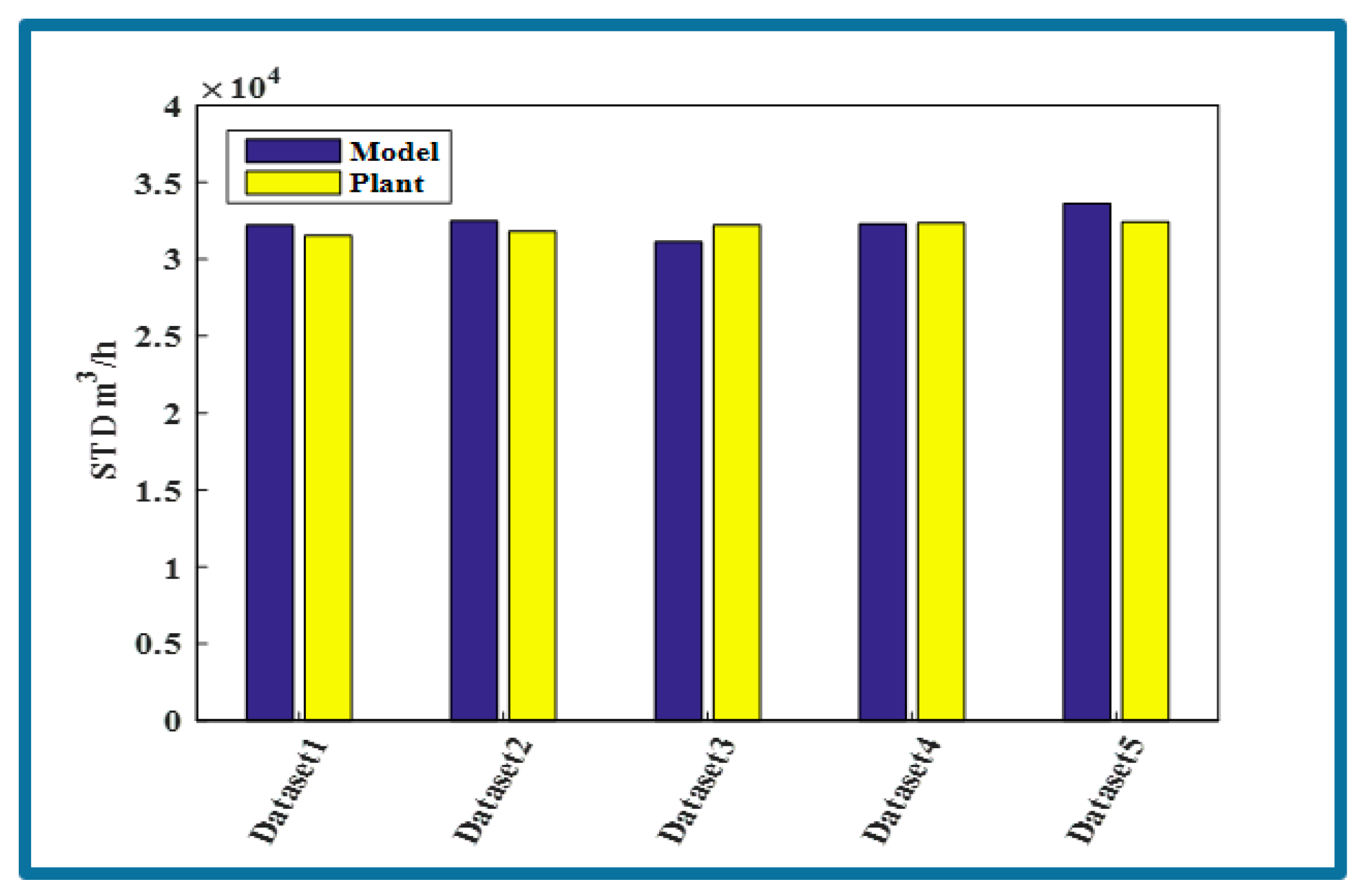
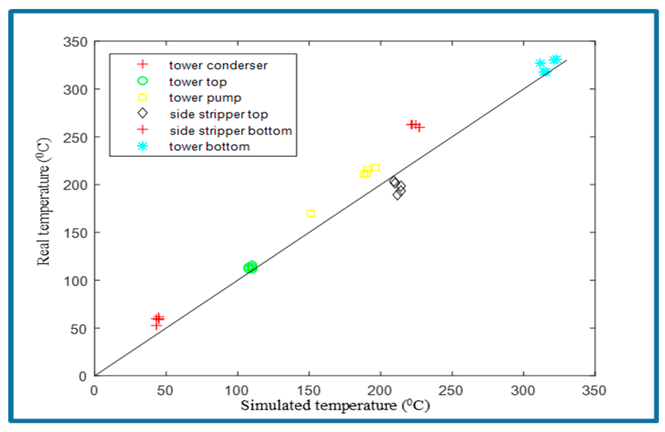
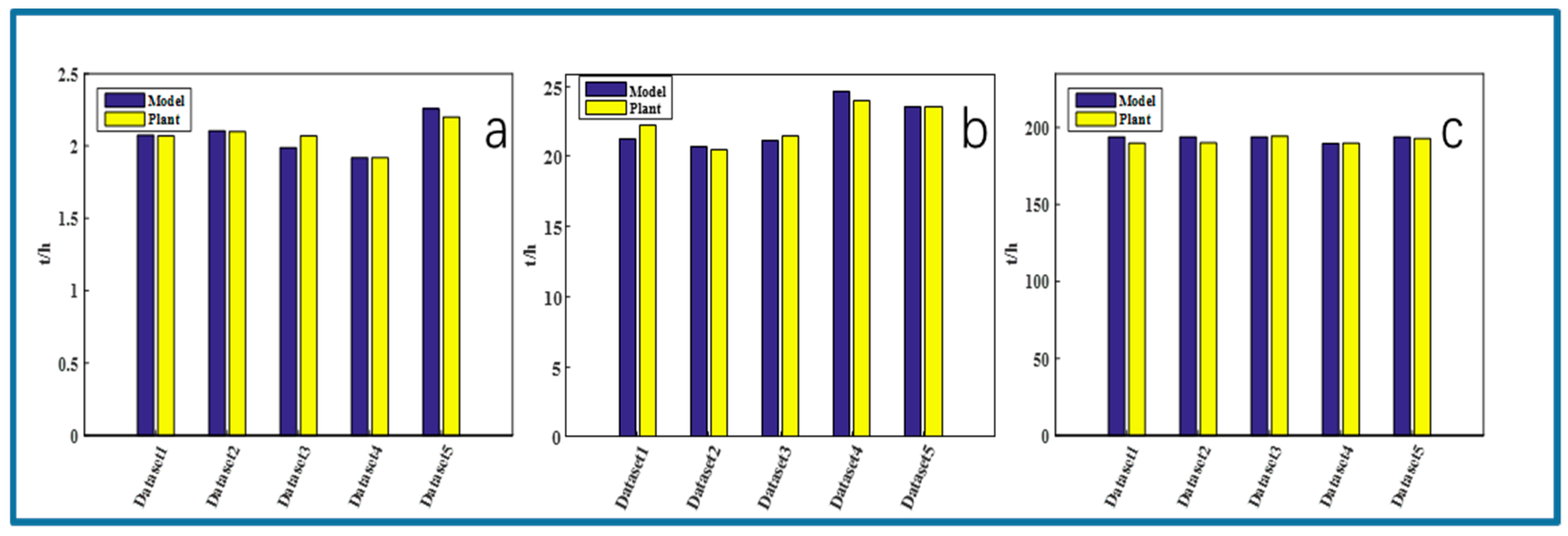
After feedstock mixture characterization, the next step is to develop reactor model. First, the process data (e.g., catalyst loading, feed rate, feedstock analysis, reactor inlet temperature, and reactor pressure) is adopted to synchronously identify the parameters of the rate equations and reactor design equations. Then, the deviation of model prediction from plant data is minimized by adjusting the reaction activity variable in the HCR model and the user-defined PFR. For the reactor model, modifying the activity factor is essential, since the feed property, reactor configuration, catalyst activity, and operating conditions differ greatly in various refineries. The procedure of adjusting the activity factor to lessen the disparity is called “calibration”. For the user-defined PFR, the kinetic parameters are identified similarly. The two parallel structure reactor model is demonstrated in
Figure 7.
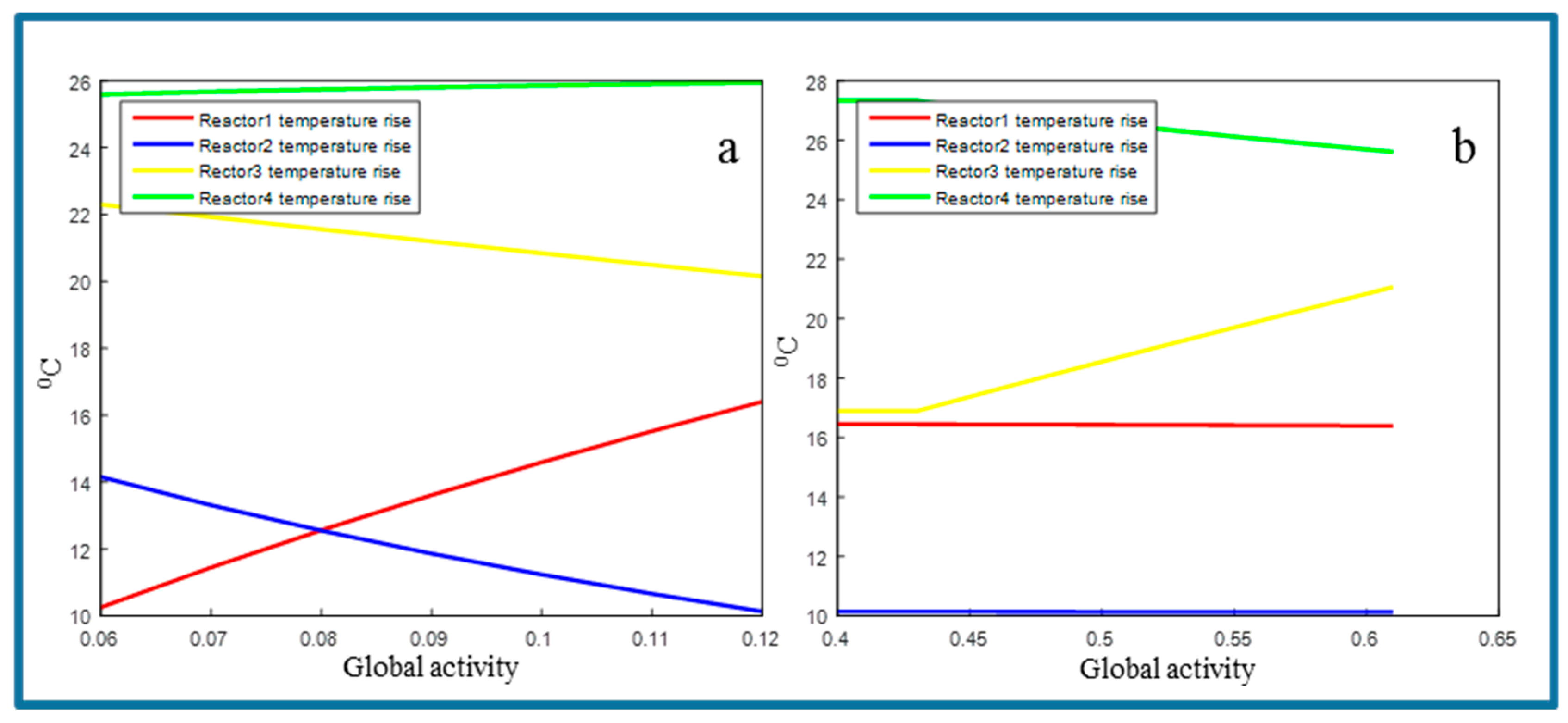
For the HCR model, the calibration procedure is already described in [
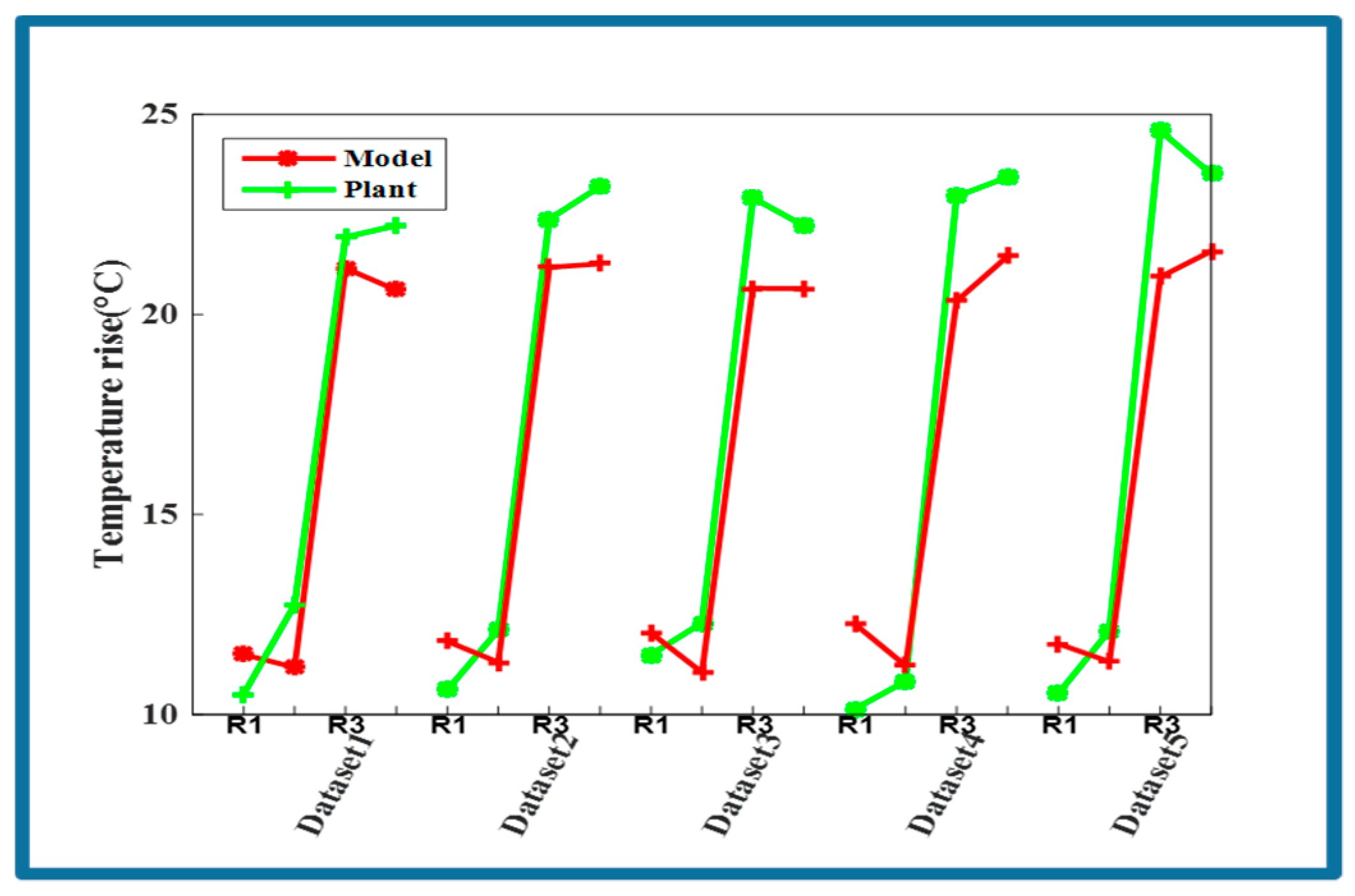
24]. Here, there are some additional steps in the calibration procedure for the residue hydrogenation process. In the tuning step, it is discovered that the reaction intensity of the catalyst bed competes against each other as shown in
Figure 8. The reaction intensity is reflected by the temperature rise since the reactions are overall exothermal. That is, when other parameters are unaltered, the global activity factor of the first catalyst bed will increase, which might result in a decline of temperature rise for the remaining catalyst bed, as demonstrated in
Figure 8. Furthermore, it is recommended that the simulated temperature rises are overall lower than the real temperature rise. It may be because the exothermal hydrodemetallization reactions are excluded in the HCR model, which occur in practical production.
Since a PFR substitutes for four reactors of the real process, the arithmetic averages of operating parameters are adopted, such as temperature, pressure, volume, and so on. For the identification of kinetic parameters, reference [
26] adopted genetic algorithm method for minimizing the deviation of the prediction of seven-lump kinetic model from the experimental data. In the established kinetic model, the activation energies were from 106.07 to 237.5 kJ. mol
−1. However, due to the deviations of the feed, operation condition between the reference and the actual process, adjustments of kinetic parameters are required to match the real process. In addition, it is impossible to directly determine the kinetic parameters for the conversion of asphaltene because the petroleum is part of the inlet residue oil in a real industrial process. To handle this problem, the consistent rule and the whole asphaltene conversion are employed. And considering the existence of a catalyst in the real process, only the activation energy is changed. The consistent rule is that the adjusted distribution of reaction activation energy should be similar to that published in [
26]. The kinetic parameters applied in this work are shown in
Table 3. It can be observed that the adjusted value is almost 0.66–0.76 times its original value.
4.3. Delumping of the Reactor Model Effluent and Fractionator Model Development
Delumping the outflow of the reactor model works as a fundamental step combining the reactor model to the fractionator model. Firstly, lumps in the reactor model are more concerned with the carbon number and structure, whereas the lumps in the fractionator model pay more attention to the accuracy of thermodynamic behavior. Secondly, the lumps used in the kinetic model belong to two different reactor models and are not integrated in this paper.
Numerous researchers have contributed to the development of this aspect. Haynes et al. [
35] applied the Gauss–Legendre quadrature to calculate the vapor–liquid equilibrium (VLE) of the petroleum whose properties are expressed by critical properties and acentric factors. Yang et al. [
36] determined appropriate fractionation lumps and their physical properties by interpolation, cutting, and normalization of the distillation curve of reactor effluent for the residue hydrogenation process. Chang et al. [
24] utilized the Gauss–Legendre quadrature to delump the overflow of the reactor model into 20 pseudo-components for the medium-pressure hydrocracking (MP HPR) and high-pressure hydrocracking (HP HPR) units.
However, a common disadvantage in these methods is that some of the related correlations are controversial. Additionally, the residue feed covers a wider range of distillation and contains more complex compositions, making the delumping tougher. Moreover, for the high and heavy fractions, property correlation may generate questionable results because the formulas are usually summarized by low boiling-point fractions. In this paper, a data-based method is applied to delump the reactor model outflow and develop the fractionator model. The component list of the method is named “Assay Components Celsius to 850 C” in ASPEN/HYSYS software. The software has collected and checked the data from the world’s most respected sources [
37]. Thus, its data source has high credibility.
Due to page limitations,
Table 4 shows only part of the pseudo-components from 340–850+C * and its property of true boiling point (TBP), ideal liquid density(ILD), molecular weight(MW). More detailed information about the complete components from 36–850+C * can be found in the
Supplementary Materials Table S1. For the distillation range from 36 to 460 °C, each temperature interval with 10 °C is represented as a lump; for the distillation boiling point range from 460 to 600 °C, approximately an interval of 20 °C was regarded as a lump; for the range from 600 to 850 °C, each interval with 25 °C is regarded as a lump; the range over 850 °C is considered as a lump. The stream cutter is adopted to connect the two models belonging to different physical property packages. The purpose of the stream cutter is to recalculate stream enthalpy. In the calculation, component A (TBP) in physical property pack 1 is mapped to pseudo-component A* in physical property pack 2 based on the boiling point.


