1. Introduction
Groundwater is simply the water found underneath the surface land, which plays a role in the hydrological cycle [
1]. It has been the most important source of fresh water used in many aspects of life such as in agriculture, irrigation, industrial processes and domestic supplies. It is usually recharged naturally due to infiltration from rains and snow melt and, to some extent, by surface water such as rivers and lakes. According to the environmental protection agency in the United States, over the last 50 years, rainfall levels have been decreasing vigorously in many areas, therefore, leading to a decrease of natural recharge of groundwater [
2].
The process of natural groundwater recharge occurs when precipitation on land surface percolates into soil and reaches the water table. Several factors must be considered when choosing the location for this process such as the characteristics of the soil and its texture, the required space, percolation rates, aquifer type, geological formations overlying the aquifer and silt control. All the factors contribute to how successful the recharge levels will be in terms of the time taken for the water to infiltrate to the aquifer, whereas heterogeneous soils would increase the time and distance for water to reach the aquifer. Additionally, temperature has a direct effect on infiltration rates where areas which encounter big differences between winter and summer have very low infiltration rates compared to the summer season [
3]. However, in summer, clogging usually occurs due to biological factors, leading to low infiltration rates.
The estimation of groundwater recharge has been a very difficult task in hydrology. Water moves within the hydrologic cycle along many complex pathways over a wide variety of time scales. The challenge for humans is to monitor the hydrologic cycle. Water budget states that the difference between the rates of water flowing in and out of an accounting unit is balanced by a change in water storage: Flow In − Flow Out = Change In Storage. The Water Budget Equation is simple, universal, and adaptable because it relies on few assumptions on mechanisms of water movement and storage. A basic water budget for a small watershed can be expressed as:
where
P is precipitation,
Qin is water flow into the watershed,
ET is evapotranspiration (the sum of evaporation from soils, surface-water bodies, and plants), Δ
S is change in water storage, and
Qout is water flow out of the watershed.
Precipitation can be written as the sum of rain, snow, hail, rime, hoarfrost, fog drip, and irrigation. Water flow into or out of the site could be surface or subsurface flow resulting from both natural and human-related causes. Evapotranspiration could be differentiated into evaporation and plant transpiration. Evaporation can occur from open water, bare soil, or snowpack (sublimation); plants can extract ground water or water from the unsaturated zone [
4]. All of this makes the complexity and uncertainty part of the equation.
Soil water balance method is an application of the water budget equation for estimating recharge often under most condition. The recharge is estimated as the residual of all the other fluxes in the hydrological cycle, the rationale being that all these fluxes (i.e., precipitation, evapotranspiration, runoff, irrigation and soil moisture changes) are usually relatively more easily measured or estimated than the recharge. Therefore, considering a volume of balance water in the root zone, the recharge
Re is estimated from:
where
I is irrigation,
RO is runoff [
5] and all other symbols have been defined previously. Yet, it is clear that the results from this equation have limited significance without calibration and validation and that is because of the substantial uncertainty in its inputting data. The equation parameters do not have a direct physical representation, which can be properly measured, in the field. At the same time, the equation parameters are indirect relation with other natural phenomena that can be easily collected from the field as rainfall, temperature, humidity, sunshine hours, and wind speed.
The fuzzy logic approach, also known as the grey box modelling, has been introduced as a solution and has been used in real-world systems where the relationship between variables is very complex or difficult to identify [
6]. This is performed by using fuzzy IF THEN rules where any object can be given a condition between ‘0’ and ‘1’ rather than the classical or ‘crisp’ set, which would either have an integer of ‘0’ or ‘1’. Adaptive Neuro-Fuzzy Inference System (ANFIS) is an approach used to model the recharge process in a similar way of human thinking and reasoning. It is a combination of fuzzy logic and neural networks introduced by Jang [
7]. This approach proved to be flexible and accurate in modelling complex, nonlinear systems since it has the ability to deal with large sets of data inputs and can provide more accurate and reliable results in comparison to other simulation and numerical-based models. More details can be found in [
8,
9,
10].
This paper will work on the approach of using fuzzy logic to reduce the uncertainties involved in the measurement of groundwater recharge by handling input data in a more simple and efficient manner. Since the water budget method involves data that is already available, it has been decided to use its parameters to attempt obtaining more accurate and reliable results. It aims to test the performance of ANFIS on a set of variables in modelling unconfined groundwater recharge using a set of data records, as well as investigating the effect of different membership function types on results.
2. Materials and Methods
2.1. Geology and Location of the Case Study
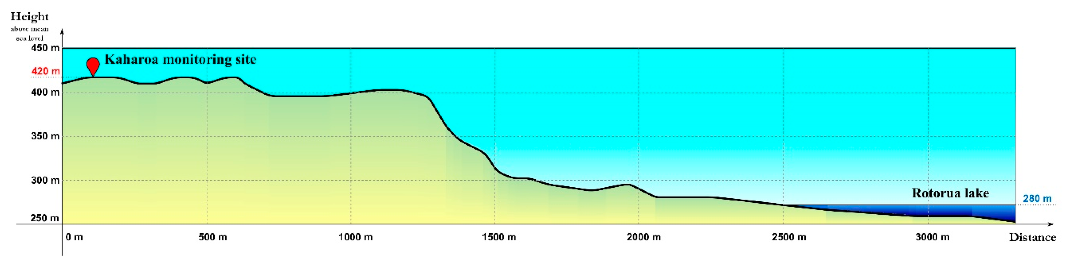
The data used in this study were from Kaharoa, it is in the Bay of Plenty region, North of Rotorua lake located in the North Island of New Zealand, it distances about 30 km from Rotorua city. The Kaharoa monitoring site has a Global Positioning System (GPS) of latitude −38.012296° and longitude of 176.268337° on map and on an elevation of 420 m above sea level at a distance of about 2.3 km from North Rotorua, the water level in the lake is around 280 m above sea level [
11].
Figure 1 illustrates the elevation section.
The Kaharoa site overlays the Mamaku Ignimbrite, which is a type of rock unit that was caused from the eruption of a magma chamber in the Taupo volcanic zone now known as The Rotorua Caldera, having a formation of 145 km
3 in volume. The soil type of the site is classified as “Orthic Pumice Soils” and more specifically the “Oropi” soil series name [
12]. Oropi soil series occur on flat, rolling and hilly uplands south of Te Puke and Tauranga and North of the Rotorua Caldera. This soil is characterized by low nutrient levels, strong leaching, sandy coarse texture which is well drained. Pumice soils in the Bay of Plenty Region, are dominated by pumice or pumice sands typically with a low clay content (<10%). Summer drought is a dominate characteristic. The soils are derived from the Kaharoa and Taupo Tephra overlaying rhyolitic tephra. They occur under an annual rainfall of 1900 to 2400 mm annually [
12].
The specific physical properties of the pumice soils in the region are [
12]:
Texture: Sand, Topsoil clay content: 5–10%;
Drainage class: Well-drained;
Permeability: Rapid;
Profile total available water (0–100 cm): Moderate to high (139 mm);
Profile readily available water (0–100 cm): High (87 mm);
Topsoil bulk density: 1.18 g/cm3;
Subsoil bulk density: 0.84 g/cm3.
The precipitation rates used in this study were collected at Kaharoa monitoring site by GNS Science under the supervision of the Bay of Plenty Regional Council. The site measures and records rainfall and rainfall percolation, collects soil water samples, besides analyzing the quality of the soil water that recharges the groundwater in Kaharoa.
2.2. Kaharoa Monitoring Site Installation
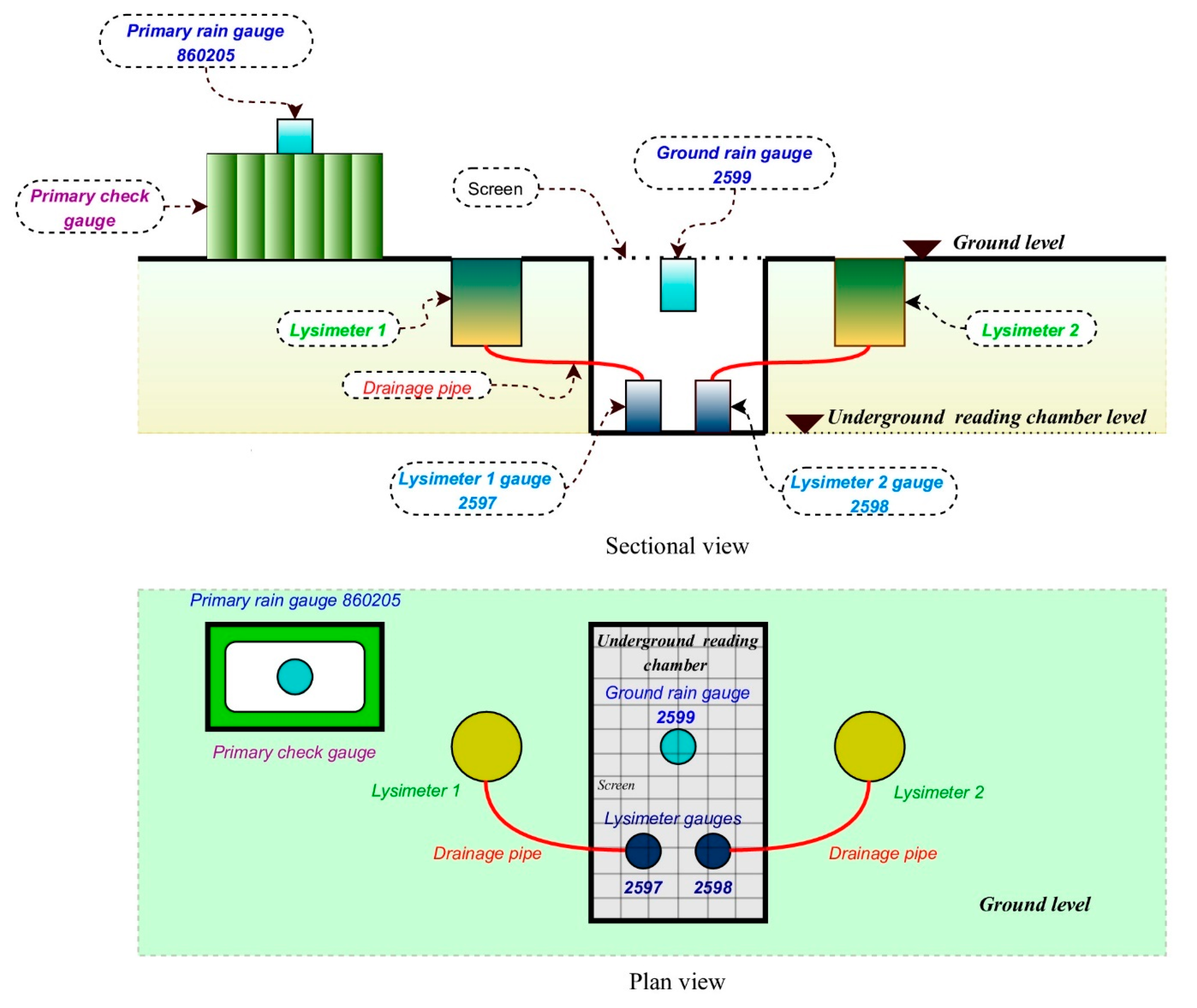
Kaharoa monitoring site was established directly beside an old rainfall recording site which has been the primary rain gauge under the number of [860205] (conventional elevated rain gauge), the site is shown in
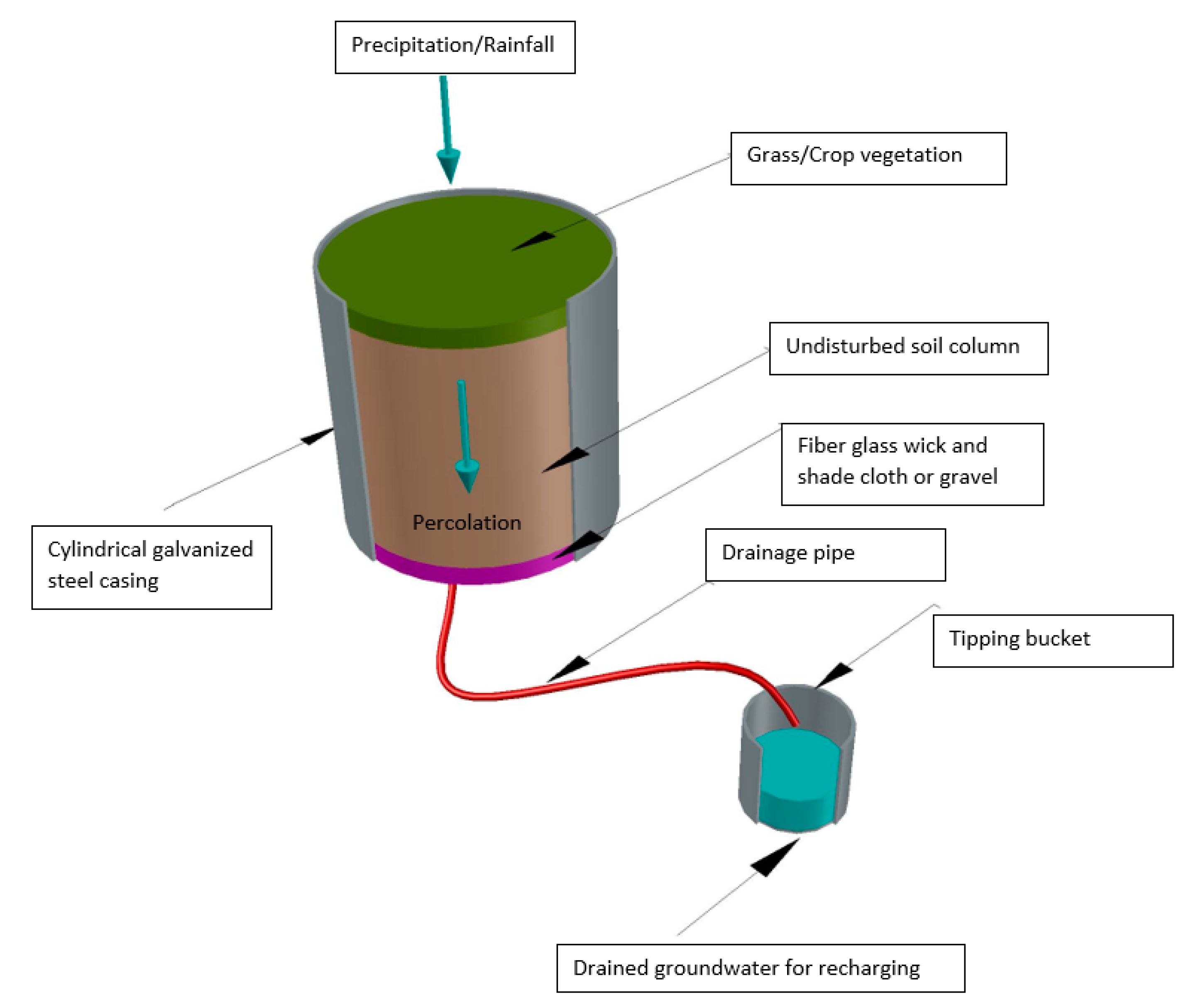
Figure 2 showing a closer look of the lysimeters. The site consists of another two non-weighing cylindrical soil monolith lysimeters, also known as percolation lysimeters, of a 500 mm diameter and a 700 mm depth and are constructed of galvanized steel connected to pipework made of polyethylene. The lysimeters are named under the number [2597] and [2598], as well as a ground-level rain gauge numbered [2599] in which a tipping bucket is attached to it to measure percolation and for real-time data collecting as demonstrated in
Figure 3. The data captured were reported to be reviewed monthly, seasonally, and annually concerning a level of rainfall and rainfall recharge at Kaharoa [
13].
2.3. Lysimeters in Groundwater Recharge
In general, a lysimeter is a device used for measuring the amount of actual evapotranspiration released by plants, usually crops. More specifically, it is a device that isolates a volume of soil between the soil surface and a given depth and includes a percolating water sampling system at its base [
13].
The soil–water balance is the simplest method when dealing with lysimeters and has been used to represent the relationship between input and output. An ANFIS model has been prepared showing the relationship between input and output using a set of existing training data packages, which will then be used as a future prediction tool. Refer to
Section 2.6 regarding ANFIS for more detail. The main soil–water balance method in determining the evapotranspiration is shown in Equation (3) [
14].
where
ET is Evapotranspiration;
I is Irrigation;
P is Precipitation;
RO is Runoff;
CR is Capillary rise (upward the root zone in case of shallow water table existence); Δ
SF is subsurface flow (horizontally inflow to or outflow of the root zone); Δ
SW is soil water content (moisture content, soil–water storage).
However, the use of lysimeters in this study has eliminated some of the parameters in Equation (3), like (I) irrigation, as the area under study is a rural pastoral grassland which depends on the rainfall only in vegetation process; (ΔSF) subsurface flow for in and out flow are stopped because of the shape of the lysimeter structural design using bounded cylinder casing; additionally, the non-existing of the shallow groundwater table makes the upward (CR) capillarity rising are not found and the rarely availability of (RO) runoff.
Thus, the previous equation can be reduced as shown in Equation (4):
The Kaharoa monitoring site records the precipitation (rainfall) and the drainage discharge (recharge) for groundwater daily. However, the full records are presented monthly as changes in soil water content (water storage) are not seen to be significant. The differences between the precipitation and drainage explain the losses in the water due to the evapotranspiration and changes in moisture content combined by using the free drainage lysimeter system, whereas the weighted lysimeter makes the assurance of the evapotranspiration values and moisture content hard to obtain. Depending on the knowledge of the precipitation and drainage or, in other words, the rainfall and recharge groundwater, and in the non-presence of other parameters, it was recommended to use the fuzzy logic techniques for forecasting the recharging water based on the available lysimeter records.
2.4. Data
The rainfall recharge site recorded monthly readings collected over 5 years, starting from December 2005 till May 2010. The site collects rainfall and recharge with two rain gauges [2599860205] and two recharge gauges [2597 and 2598]. The recharge gauge [2598] was eliminated due to its inaccuracy where a leakage was observed. The Kaharoa site is classified as a rain gauge data collector that can take records on an interval of 15 min, which can easily monitor events even for short-term rainfall. Therefore, it was preferred to use the ground rainfall gauge [2599] over [860205] as it is relatively very near to lysimeter’s location and it imitates the same amount received; thus, the record readings in [2599] for rainfall is taken in consideration with lysimeter [2597] for recharge in this study.
The data record had to be divided into three packages: a package for ‘Training data’, ‘Validation or checking data’ and finally for ‘Testing data’. These data were not enough for generating a proper fuzzy logic model as more variables are needed to improve the performance of the model in predicting the groundwater recharge. Temperature in Celsius degree, relative humidity and sunshine in hours, published on the certified environmental New Zealand official site, 2019, was used to support the modelling exercise. These data readings were noted to be mean monthly values ranging from the year 1981 till 2010 for the location under study having a minimum of five full-year data and scheduled yearly by monthly sequence starting from January till December.
A 53 data readings were divided into three sets. The first 29 readings starting from December 2005 till April 2008 were used for training, 12 readings starting from May 2008 till April 2009 were used for validation (checking) and last 12 readings which starts from May 2009 till April 2010 were used for testing, as shown in
Table 1.
The average recharge to rainfall was around 40% per month, reaching a maximum of 121% in August 2008 (more research to be conducted for the reason behind this as this out the scope of this study, but they are kept as the fuzzy model could eliminate their effects) and minimum of 0% which happened several times as counted 11 times for 53 records. Firstly, in February 2007 and lastly in March 2010, twice in 2007, three times in 2008, four times in 2009 and, lastly, two times in the uncompleted year 2010. That might indicate the reason behind the temperature rising and less rainfall.
Figure 4 illustrates the regression comparison between the input parameters and the output parameter (recharge) as in
Figure 4a, shows that the rainfall to recharge R
2 = 0.699 that is a fairly linearly; however, the regression for the other input parameters temperature, relative humidity and sunshine hours represents (R
2 = 0.24, 0.35 and 0.25) a non-linearity nature.
2.5. Fuzzy Logic Inference Systems
Fuzzy logic systems are non-linear mapping of the input space to the output space, where the input is first converted from a crisp integer to a fuzzy value, known as ‘fuzzification’ through the use of membership functions [
15]. It is then processed through a set of fuzzy rules. The output for each rule is then converted from fuzzy to a crisp value, this process is known as ‘defuzzification’. The main components used in this system are fuzzy-sets, membership functions, fuzzy IF-THEN rules and fuzzy-logic operators.
There are two main types of fuzzy inference systems that could be used, the first inference system is called Mamdani’s fuzzy system [
15]. The second one is known as Takagi-Sugeno-Kang inference system (TSK) [
16]. Mamdani’s inference system relies that the consequent membership functions are fuzzy in nature and all the system is totally fuzzy starting from input, fuzzy rules and output variables. The Sugeno method is another approach for generating a set of fuzzy rules for a given input–output data. It is the same as the Mamdani method, however, the difference comes in the consequent part, which consists of linear or constant membership functions rather than fuzzy sets. Overall, Sugeno inference has been recognised to be flexible, more effective than Mamdani inference due to its efficiency in data processing and simplicity in the defuzzification.
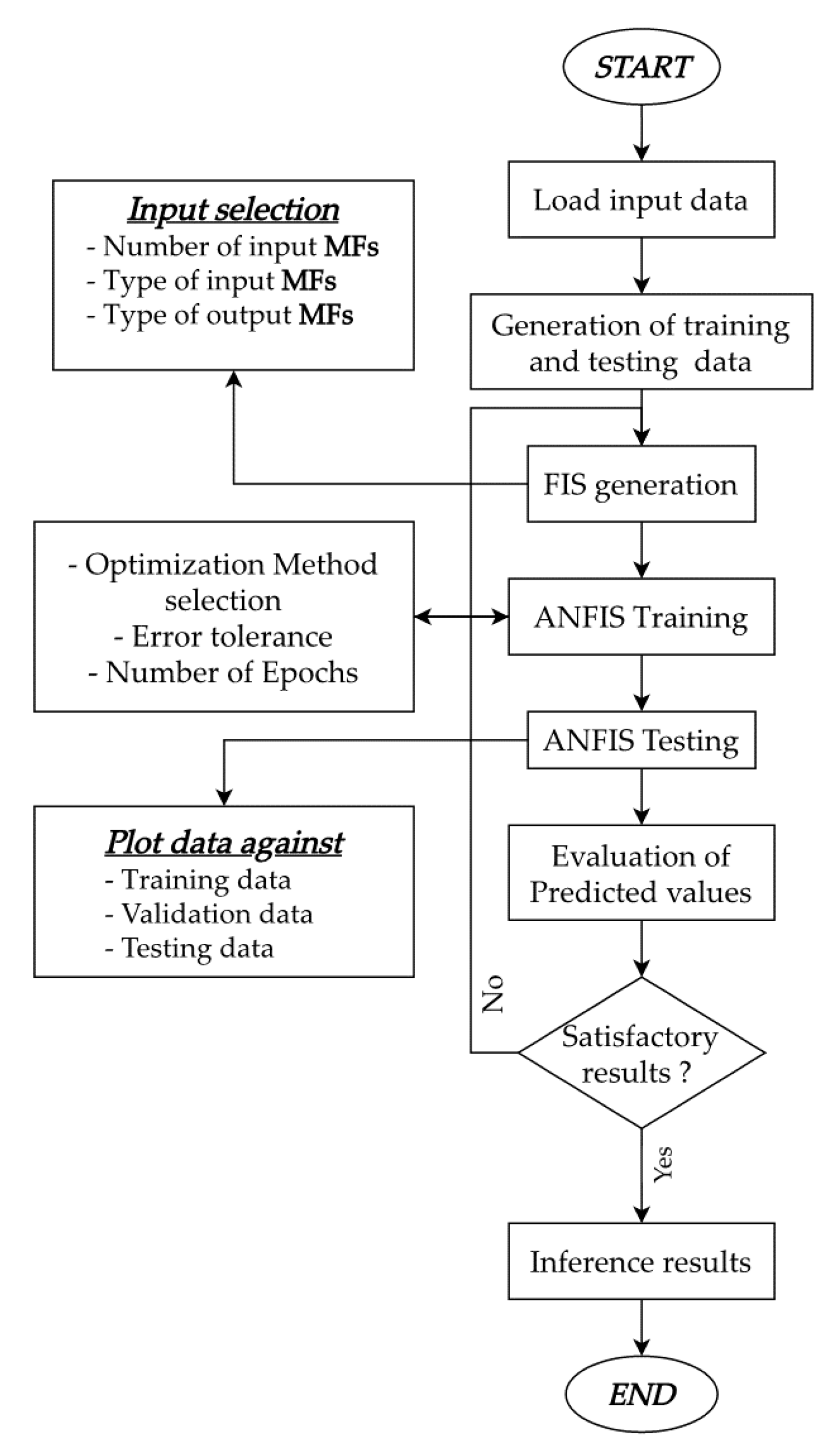
The Adaptive Neuro Fuzzy Inference system (ANFIS), which is chosen in this paper, is a graphical representation of the Sugeno inference system embedded with neural network learning capabilities, where each output per rule can be linear or constant functions [
17]. It provides an optimization method for dealing with the parameters in the fuzzy system that best fit with the input data. The diagram in
Figure 5 illustrate the ANFIS model.
2.6. Modeling Framework
The fuzzy logic toolbox in MATLAB (Version 9.5 (R2018b), MathWorks, Natick, Massachusetts, United States, 12 September 2018) [
18] was chosen for this study. Sugeno type was chosen using the ANFIS. Initially, four main input parameters were chosen, rainfall, temperature, relative humidity percentage and sunshine hours. Relative humidity percentage was used to express the effect of evaporation and evapotranspiration, Sunshine hours to express the effect of solar radiations, whilst recharge was the output value. Gaussian membership function was used for the input space while linear membership function was chosen for the output space. For parameter optimization, hybrid method backpropagation was used, and the error tolerance was sat as Zero and the number of epochs was set to avoid over fitting of the model. The best structure of the model, the number of inputs and the number of memberships function, was found by trial and error in order to get the best model performance using the performance evaluation criteria.
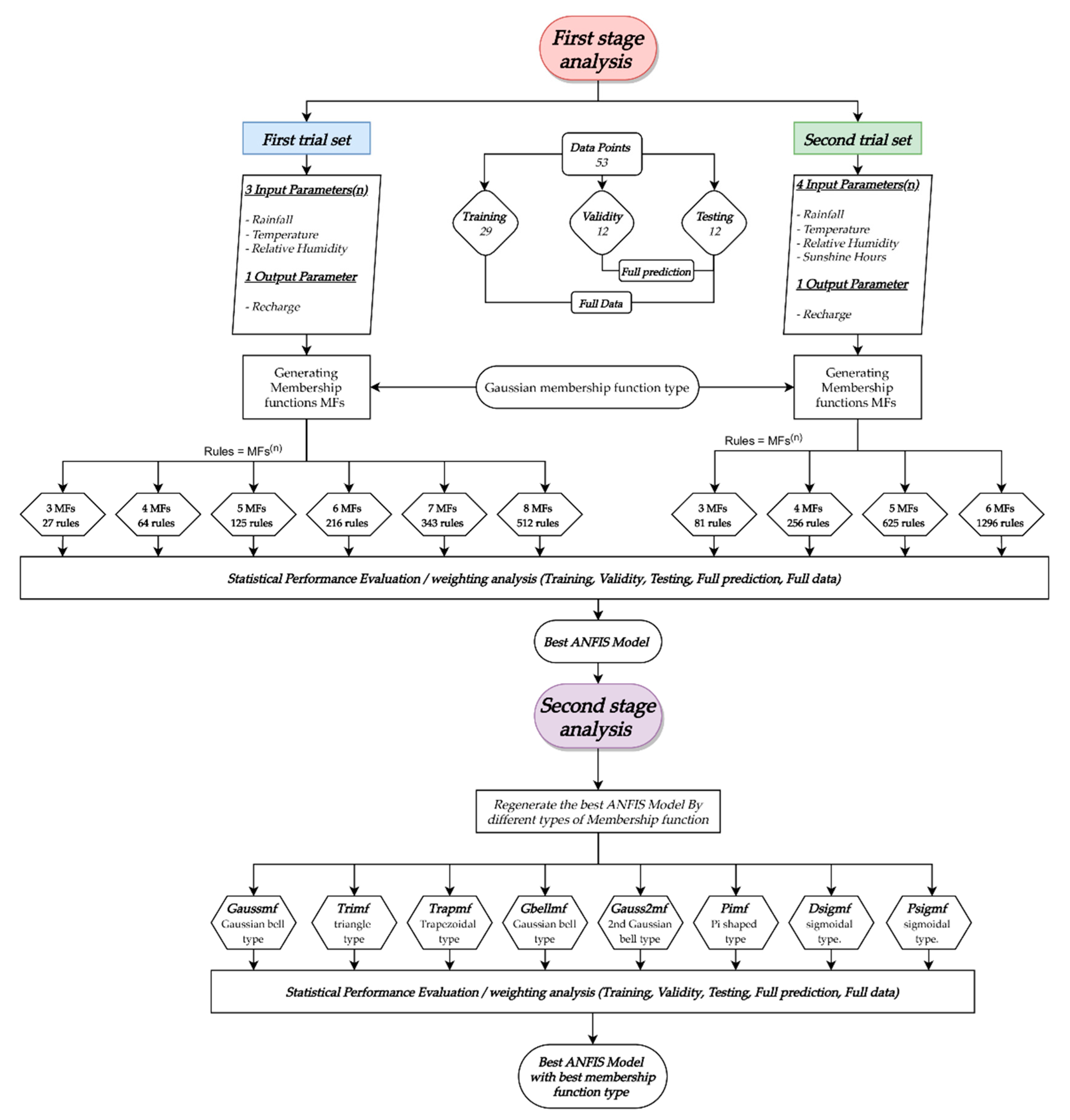
The study is divided into two stages, the first stage aims to get the best ANFIS model from a limited number of input parameters by changing the number of membership functions and keeping the type of the membership function constant, while the second stage aims to get the best membership function type that increases the performance of the best ANFIS from the first stage by examining the different types. Available data points were divided into 3 parts, 29 data points are used for training, 12 data points are used for validation and checking, and 12 data points are used for testing.
The outputs of the ANFIS model are compared with the observed readings from the field (the lysimeter gauges records) to see how far the outputs are related to the field and how much is the error weights, by using several statistical methods. These statistical methods elect the most adapted ANFIS model that could be as nearest as the recorded field reading with less error differences.
The number of input parameters to be estimated in the ANFIS can be very large. For example, depending on the number of input parameters and the number of membership functions for each input, and the shape of membership function chosen, the total number of parameters is estimated by Equations (5)–(7) [
19].
where
Ntotal = Number of modified parameters, i.e., to be estimated;
Ninput = Number of input parameters;
Nmf = Number of membership functions associated with each input;
Npp = Number of modified parameters per membership function, i.e., 2 in the case of Gaussian membership function;
l = Number of rules;
Ncp = Number of modified parameters in the sequence part of each rule.
The first stage of analysis consists of two trial set models, the first trail set is conducted with ANFIS using MATLAB for three inputs (rainfall, temperature, and relative humidity) and recharge as an output having 3 to 8 Gaussian membership functions generating 27 rules as starting up with three membership functions to 512 rules with 8 membership functions, while the second trail set measures the effect of adding the sunshine hours as the 4th input variable parameter to the ANFIS model and keeping the previously used sequence, starting with 3 to 6 membership functions of the Gaussian type generating 81 rules as starting up to 1296 rules.
The second stage of analysis aims for more refining and perfection for the ANFIS model and for studying the effect of changing the type of the membership function on the outputs. The first stage assumption for the membership function type was Gaussian type; in the second stage, it was replaced by other types of membership functions in which it have to be checked versus all other types through ANFIS modelling; the other types used in this study are tri
mf (triangle type), trap
mf (trapezoidal type), gbell
mf (Gaussian bell type), gauss2
mf (2nd Gaussian type), pi
mf (Pi shaped) and dsig
mf (difference between two sigmoidal functions).
Figure 6 shows a detailed structure of the two-stage analysis for a better understanding of the overall model.
2.7. Performance Evaluation Criteria
The model has been evaluated using several evaluation criteria such as correlation coefficient (R), mean squared error (MSE), average absolute error (AAE), root mean square error (RMSE), and coefficient of efficiency (CE). More details on these criteria can be found in [
19,
20].
3. Results
In the first stage of analysis, two trial set models have been developed. The first trial set model used three input parameters, whereas the second trial set model used four input parameters, both used different numbers of Gaussian membership functions. The performance of these models in predicting recharge (the lysimeter gauges records) is presented in
Table 2.
The training set yield relatively the same values for the observed, however the differences are clearly noticed in the validation and testing sets in comparison to the observed. At the same time, it expresses some limitations that must be taken into consideration for future improvements, these improvements must include more readings and data entry as the more values for the training set the more output perfection.
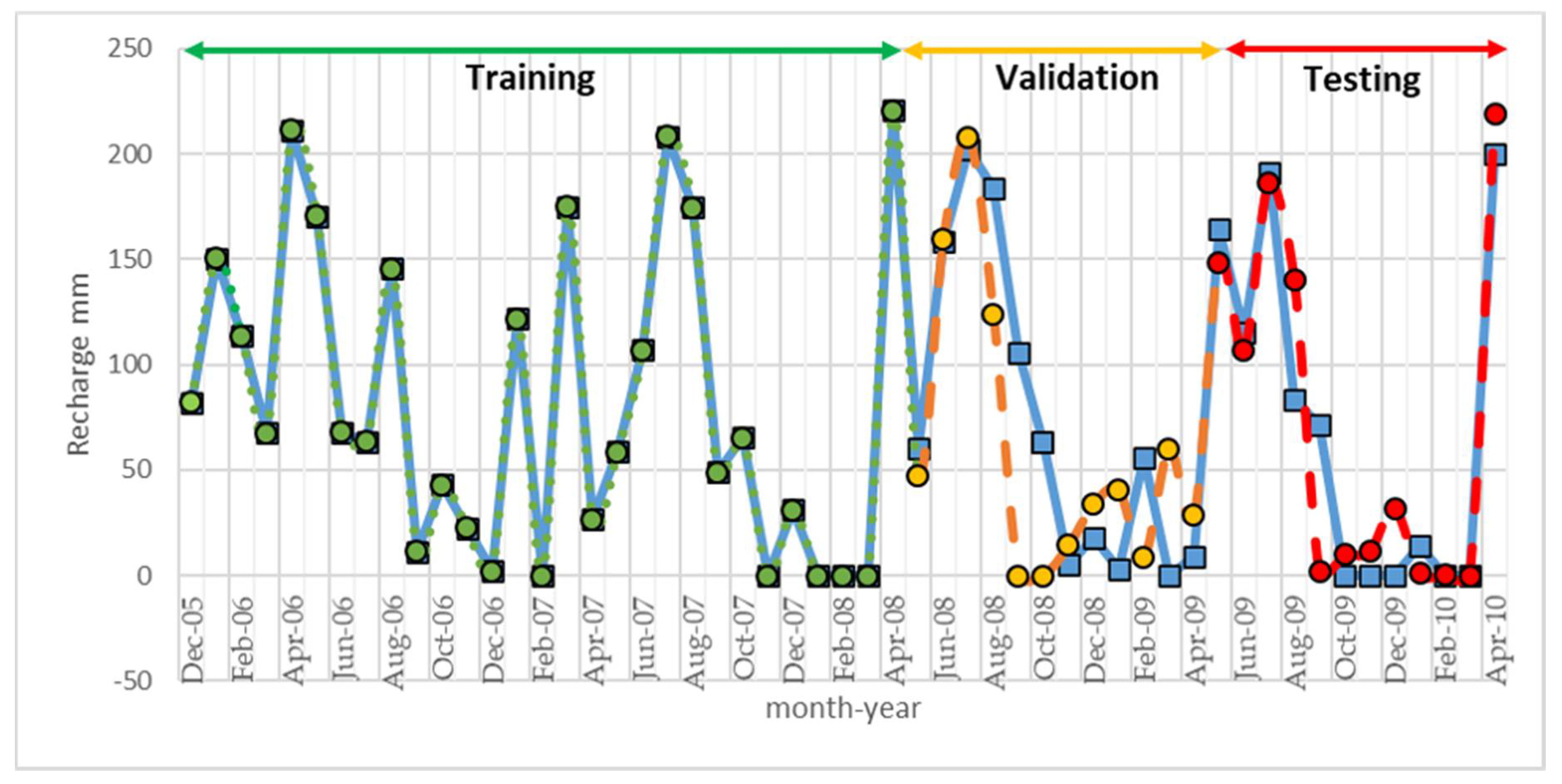
By comparing the developed models, it is found that three input parameters with seven membership functions generate the best performance.
Figure 7 shows the comparison between predictions observed during training, validation, and testing.
The number of parameters used is a solid part of the ANFIS modelling, more effective variables equals more accuracy and imitation of the real filed observation. The first trial set was concerning three constant numbers of parameters (rainfall, temperature and relative humidity), equally incrementing the number of membership functions for each parameter, while the second trail set was concerning four parameters instead of three parameters by adding the parameter of sunshine hours. Despite increasing the number of parameters and that the ANFIS models generates a greater number of rules, the best model came in the first trail set, three parameters and seven MFs. This was due to the fact that the “sunshine hours” parameter was noticeably in the same range as the temperature parameter, therefore giving the same meaning with not much effect on the output.
For more refinement and perfection of the ANFIS model, and for studying the effect of changing the type of the function on the outputs, the previous assumption for the membership function type as Gaussian have to be checked versus all the other types that can be used through ANFIS modelling, as trimf (triangle type), trapmf (Trapezoidal type), gbellmf (Gaussian bell type), gauss2mf (2nd Gaussian type), pimf (Pi shaped) and dsigmf (Difference between two sigmoidal functions). This is implemented in stage 2 analysis. The performance of different models using correlation coefficient is shown in
Table 3.
As seen from
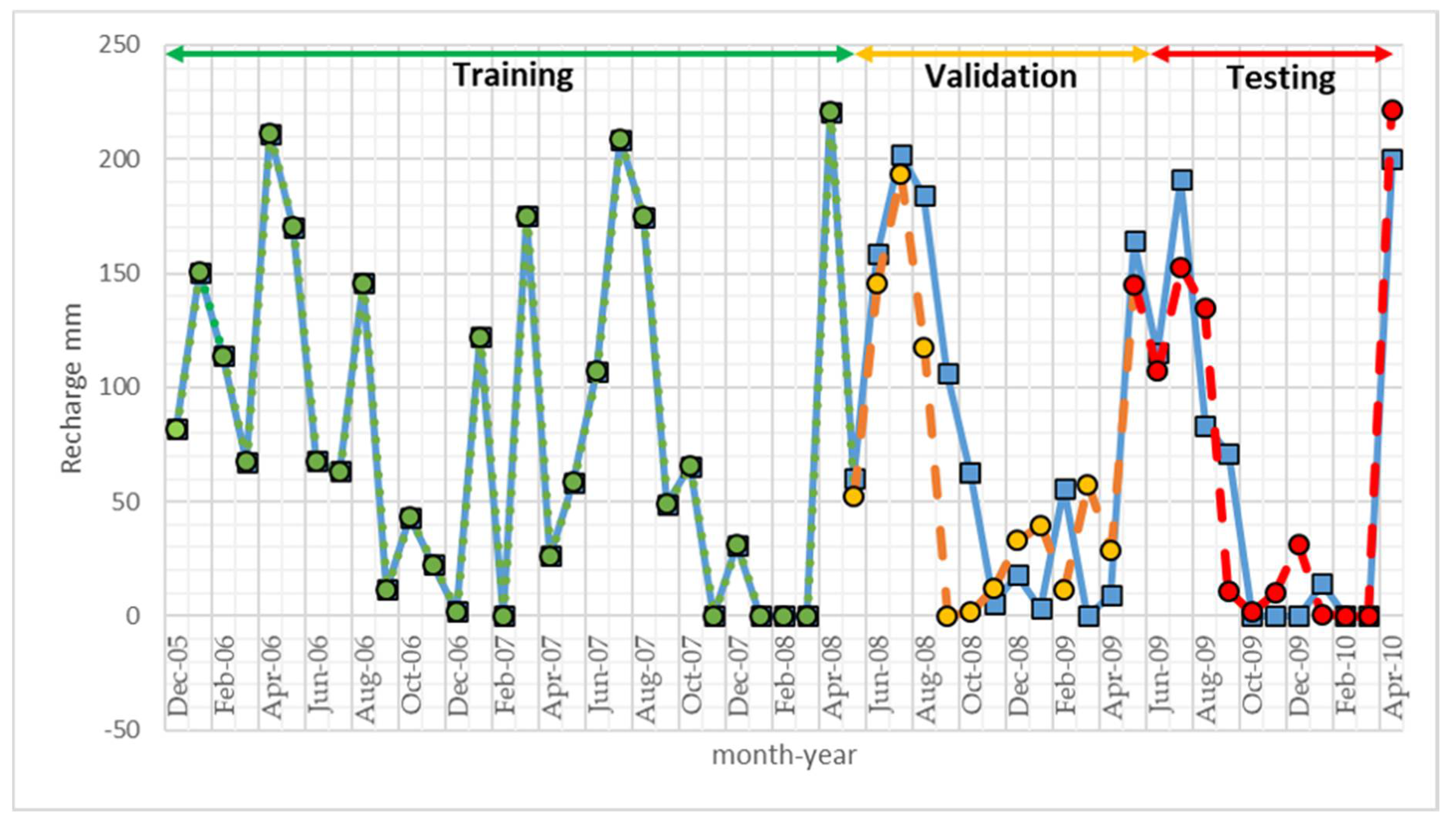
Table 4, the tri
mf (triangle) membership function type was the most statistically agreed on by 13/20 or 65% of all the comparisons; however, the differences between it and the Gaussian type is relatively small and the same for trap
mf, pi
mf and gauss2
mf, yet it was touchable in comparison to dsig
mf, psig
mf and gbell
mf.
Figure 8 illustrates the performance of the best model 3 × 7Mfs type Trimf.
4. Discussion
Predicting groundwater recharge in the past has been a very difficult process when using the traditional deterministic methods due to its complexity and uncertainty of data; therefore, the use of artificial intelligence techniques was seen to be the most successful in the estimation of groundwater recharge due to the fact that it can handle large amounts of data in a simple manner, with no prior knowledge of the structure of the system. However, these techniques depend greatly on the quality of the data provided.
This work attempted to test the hypothesis that AI techniques can significantly help in forecasting future readings by minimizing the maximum prediction error rates and reducing the uncertainties involved by handling input data in a more simple and efficient manner. The main aim was to use ANFIS to predict the groundwater recharge using some easily measured parameters such as temperature, rainfall, relative humidity and sunshine radiation. Other objectives included investigating whether or not the number of input parameters have a direct effect on the results. Additionally, to investigate the effect of different membership function types on the results. The benefits and merits of using ANFIS modelling for predicting groundwater recharge and the obtained results corresponding to our objectives are discussed in the following paragraphs.
The paradox of prediction of groundwater recharging theoretically requires measuring of many parameters which may be unmeasurable or difficult to ensure. The use of ANFIS model with a few numbers of easy measurable parameters provides us with significant results. For example, with the help of 29 readings of 3 parameters, 3 membership functions in training set, 52% is reached as a correlation coefficient (R) for a total set of data as a starting point. Moving to the best ANFIS model, three parameters and seven membership functions, the correlation coefficient increased to be 93% for the total set, 77% for the validity set and 93% for the testing set.
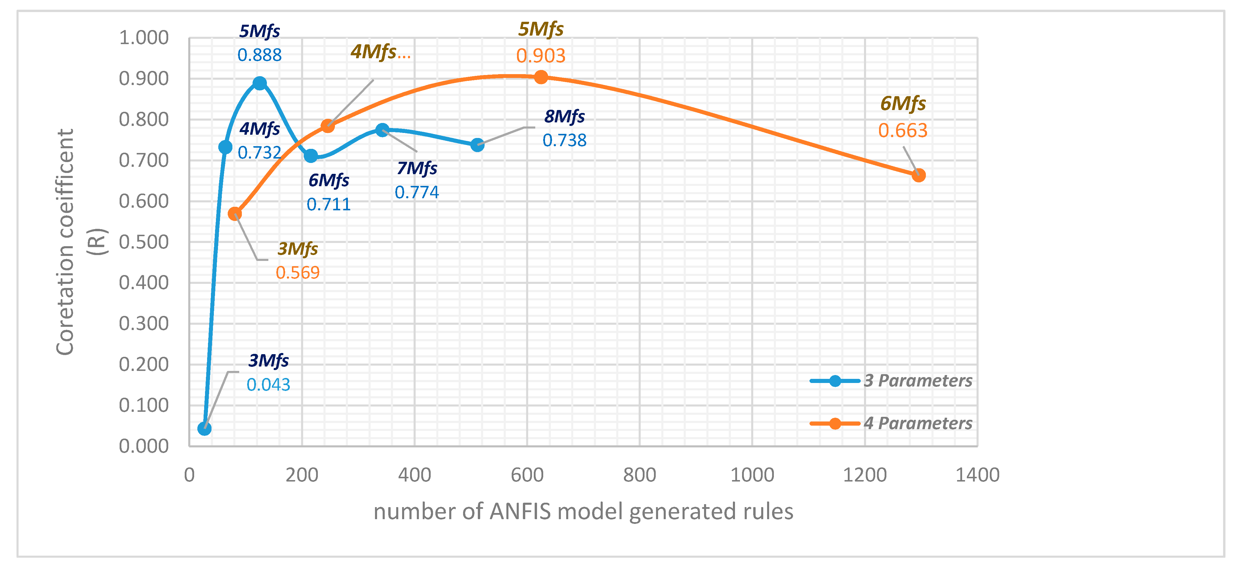
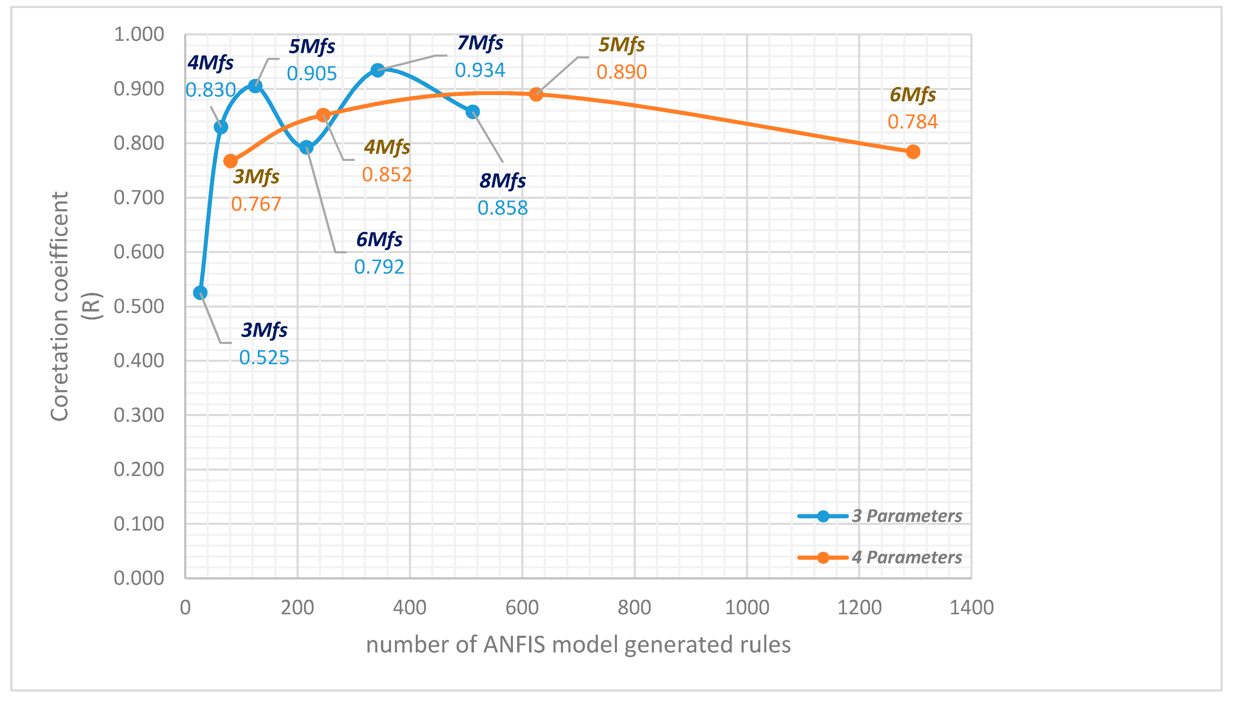
For more investigation,
Figure 9,
Figure 10 and
Figure 11 show the relation between the correlation coefficient (R) and ANFIS model number of generated rules. They reveal the fluctuation of the three-parameter models which start with a low range, and then increase with increasing number of membership functions in the mentioned three sets. In the four parameters, the curve rises gradually to a peak before then fallings down gradually. Here, the curve could either move upwards, which is less likely, or continue moving downwards. Hereby, the idea of the added fourth parameter may not be as effective as expected; thus, the choice of parameters greatly depends on the quality of the data and how strong and effective it is in connection to the point of study rather than the number of parameters.
ANFIS modelling contains eight different types of membership functions with different behaviors for the same number of parameters and number of membership functions, the second-stage analysis in the study highlights the importance of the type of the membership functions used in modelling. The type of the curve was established to be Gaussian type (gaussmf) as an assumption, eventually a comparison is driven between different types to assure the type for the best ANFIS model. Changing of types can make a direct impact on the output values. In this case, the superiority of the trimf type on the gaussmf is not that much remarked.
The findings appear to be consistent with other AI techniques applied to groundwater recharge estimations. For example, Umamaheswari and Kalamani [
19], who tried to develop the best ANFIS model that could reflect the groundwater fluctuation based on four input parameters as duration, groundwater recharge and groundwater discharge, and monthly groundwater level as output, had results showing that R
2 gives 0.921, CE gives less than 0.1, CC gives more than 0.96, MSE gives less than 0 and RMSE gives 0.3. These results are very close to the results found from this paper where R
2 was 0.865, CE was 0.86, CC was 0.93, the rest of MSE and RMSE are not applicable for comparison.
In comparison to another work by Raghavendra and Deka [
21], who also compared two methods for prediction of groundwater recharge using ANFIS and GPR (Gaussian Process Regression) modelling based on two wells, our results were clearly better than their findings when comparing the performance evaluation for ANFIS models. The work expressed good results as NSE was 0.86, while their research gave 0.82 as maximum and 0.71 as minimum value. For CC, these results gave 0.93, while their research gave 0.85 as maximum and 0.75 as minimum value. These differences could be due to different time periods being used as well as different types of parameters involved.
The ANFIS modelling is a highly talented artificial technique that can solve and predict with high accuracy with no need for extensive or deep data exploration. Few parameters and data can eliminate many of uncertainties and unmeasurable data parameters.


