Dynamic Threshold Neural P Systems with Multiple Channels and Inhibitory Rules

Abstract

In biological neural networks, neurons transmit chemical signals through synapses, and there are multiple ion channels during transmission. Moreover, synapses are divided into inhibitory synapses and excitatory synapses. The firing mechanism of previous spiking neural P (SNP) systems and their variants is basically the same as excitatory synapses, but the function of inhibitory synapses is rarely reflected in these systems. In order to more fully simulate the characteristics of neurons communicating through synapses, this paper proposes a dynamic threshold neural P system with inhibitory rules and multiple channels (DTNP-MCIR systems). DTNP-MCIR systems represent a distributed parallel computing model. We prove that DTNP-MCIR systems are Turing universal as number generating/accepting devices. In addition, we design a small universal DTNP-MCIR system with 73 neurons as function computing devices.

1. Introduction

Membrane computing (MC) is a type of system with the characteristic of distributed parallel computing, usually called P systems or membrane systems. MC is obtained by researching the structure and functioning of biological cells as well as the communication and cooperation of cells in tissues, organs, and biological neural networks [1,2]. P systems are mainly divided into three categories, namely cell-like P systems, tissue-like P systems, and neural-like P systems. In the past two decades, many P-system variants have been studied and applied to real-world problems, and most of them have been proven to be universal number generating/accepting devices and functional computing devices [3,4].

1.1. Related Work

Spiking neural P (SNP) systems are abstracted from biological facts that neurons transmit spikes to each other through synapses. An SNP system can be regarded as a directed graph, where neurons are regarded as nodes, and the synaptic connections between neurons are regarded as arcs [5,6]. SNP systems are the main form of neural-like P systems [7]. An SNP system consists of two components: data and firing rules. Data usually describe the states of neurons and can also indicate the number of spikes contained in every neuron. Firing rules contain spiking rules and/or forgetting rules. The firing of rules needs to satisfy necessary conditions. The form of firing rules is $\mathrm{E}/{\mathrm{a}}^{\mathrm{c}}\to {\mathrm{a}}^{\mathrm{p}}$, where E indicates the regular expression. When ${\mathrm{a}}^{\mathrm{n}}\in \mathrm{L}\left(\mathrm{E}\right)$ and $\mathrm{n}\ge \mathrm{c}$, the rule is applied and the neuron fires. $\mathrm{L}\left(\mathrm{E}\right)$ represents the language set associated with regular expressions E. ${\mathrm{a}}^{\mathrm{n}}$ indicates that the neuron where the rule is located contains n spikes. Once the rule is enabled, the neuron removes c spikes and transmits the generated p spikes to succeeding neurons. When $\mathrm{p}=0$, rule $\mathrm{E}/{\mathrm{a}}^{\mathrm{c}}\to \mathrm{\lambda }$ is called a forgetting rule. $\mathrm{\lambda }$ represents an empty string, which indicates that forgetting rules does not generate new spikes. In summary, the firing condition of a firing rule is: ${\mathrm{a}}^{\mathrm{n}}\in \mathrm{L}\left(\mathrm{E}\right)$ and $\mathrm{n}\ge \mathrm{c}$. This means that the firing of a rule is only related to the state of the neuron and has nothing to do with the state of other neurons. Moreover, the parallel work of neurons determines that SNP systems are models of distributed parallel computing. Therefore, most SNP systems are equipped with a global clock to mark time. SNP systems also have nondeterminism characteristic. If more than one rule can be enabled in a neuron at a certain time, then only one of them will be selected non-deterministically.

Neural-like P systems have received extensive attention and research in recent years. SNP systems was proposed by Ionescu et al. [7]. Usually, SNP systems have spikes and forgetting rules, but Song et al. [8] proposed that neurons can also have request rules. The request rules enable neurons to perceive “stimuli” from the environment by receiving a certain number of spikes. Zeng et al. [9] proposed SNP systems with weights. In this system, when the potential of a neuron is equal to a given value (called a threshold), it will fire. Zhao et al. [10] introduced a new mechanism called neuron dissolution, which can eliminate redundant neurons generated in the calculation process. In order to enable SNP systems to represent and process fuzzy and uncertain knowledge, the weighted fuzzy peak neural P system was proposed by Wang et al. [11]. Considering that SNP systems can only fire one neuron in each step, sequential SNP systems is investigated [12,13]. Although most SNP systems are synchronous, asynchronous SNP systems are investigated by [14,15,16]. Song et al. [15] also studied the computing power of asynchronous SNP system with partial synchronization. Moreover, most SNP systems as number generating/receiving devices [17,18], language generators [19], and functional computing devices [20,21] have been proven to be Turing universal. Furthermore, SNP systems have applications in dealing with real-world problems, such as fault diagnosis [22,23,24], clustering [25], and optimization problems [26].

1.2. Motivation

Yang et al. [27] researched SNP systems with multiple channels (SNP-MC systems) based on the fact: there are multiple ion channels in the process of chemical signal transmission, therefore, spiking rules with channel labels are introduced into neural P systems. After SNP-MC systems were proposed, many neural P systems combine with multiple channels have been investigated. They prove that using multiple channels can improve the computing power of neural P systems.

In addition, there are the following facts in the biological nervous system:

(1)

The conduction of nerve impulses between neurons is unidirectional, that is, nerve impulses can only be transmitted from the axon of one neuron to the cell body or dendrites of another neuron, but not in the opposite direction.

(2)

Synapses are divided into excitatory synapses and inhibitory synapses. According to the signal from the presynaptic cells, if the excitability of the postsynaptic cell is increased or excited, then the connection is excitatory synapse. If the excitability of the postsynaptic cell is decreased or the excitability is not easily generated, then it is inhibitory synapse.

Li et al. [28] were inspired by the above two biological facts and proposed SNP system with inhibitory rules (SNP-IR systems). The firing condition of an inhibitory rule not only related to the state of neuron where the rule is located but also related to other neurons (presynaptic neurons). This is because of the unidirectionality of nerve impulse transmission. SNP-IR systems have stronger control capabilities than other SNP systems.

Peng et al. [29] first proposed the dynamic threshold neural P systems (DTNP systems), which were abstracted from ICM model of the cortical neurons. The firing mechanism of DTNP systems are different from SNP systems. DTNP systems adopt a dynamic-threshold-based firing mechanism, and they have two data units (feeding input unit and dynamic threshold unit) as well as a maximum spike consumption strategy. In order to improve the computational efficiency of DTNP systems, we introduce multiple channels and inhibitory rules.

The main motivation of this paper is mainly to introduce inhibitory rules into DTNP systems, which can better reflect the working mechanism of inhibitory synapses and simulate the actual situation of communication between neurons through synapses. The introduction of multiple channels improves the control capability of the DTNP system so that it can better solve real-world problems.

Compared with DTNP systems, DTNP-MCIR systems have the following innovations:

(1)

DTNP-MCIR systems introduce firing rules with channel labels.

(2)

Inspired by SNP-IR systems, we introduce inhibitory rules to DTNP systems, but the form and firing conditions of inhibitory rules have been re-defined.

(3)

The firing rules of neuron ${\mathrm{\sigma }}_{\mathrm{r}}$ (corresponds to register r) is ${\mathrm{E}}_{\mathrm{r}}/\left({\mathrm{a}}^{\mathrm{u}},{\mathrm{a}}^{\mathrm{\tau }}\right)\to {\mathrm{a}}^{\mathrm{p}}(\mathrm{l})$ in DTNP systems, ${\mathrm{E}}_{\mathrm{r}}$ is a default firing condition usually not displayed, because ${\mathrm{E}}_{\mathrm{r}}=\left\{{\mathrm{u}}_{\mathrm{i}}\ge {\mathrm{\tau }}_{\mathrm{i}}\wedge {\mathrm{u}}_{\mathrm{i}}\ge \mathrm{u}\wedge {\mathrm{\tau }}_{\mathrm{i}}\ge \mathrm{\tau }\right\}$ can be reflected in the rules. However, ${\mathrm{E}}_{\mathrm{r}}$ can also be a regular expression in DTNP-MCIR systems, for example ${\mathrm{a}}^{2\mathrm{b}+1}/\left({\mathrm{a}}^{\mathrm{u}},{\mathrm{a}}^{\mathrm{\tau }}\right)\to {\mathrm{a}}^{\mathrm{p}}(1)$, where ${\mathrm{a}}^{2\mathrm{b}+1}$, $\mathrm{b}\ge 1$ represents an odd number of spikes. The rule is only enabled when neuron ${\mathrm{\sigma }}_{\mathrm{r}}$ contains an odd number of spikes and satisfies the default firing condition.

If a rule in a neuron is enabled in DTNP-MCIR systems, then the number of spikes consumed by the neuron is $\mathrm{u}+\mathrm{\tau }-\mathrm{p}-\mathrm{n}$. When two rules in a neuron can be applied simultaneously at time t, we can choose one of the rules according to the neuron’s maximum spike consumption strategy.

Based on the above, we built a variant of DTNP systems called dynamic threshold neural P systems with multiple channels and inhibitory rules (DTNP-MCIR systems). We will prove Turing universal of DTNP-MCIR systems as number generating/accepting devices and functional computing devices. The content of the rest of this paper is arranged as follows. Section 2 defines DTNP-MCIR systems and gives an illustrative example. Section 3 illustrates the Turing universality of DTNP-MCIR systems as number-generating/accepting devices. Section 4 explains DTNP-MCIR systems as function computing devices. Section 5 is the conclusion of this paper.

2. DTNP-MCIR Systems

In this section, we define a DTNP-MCIR system, describe some of its related details, and give an illustrative example. For convenience, DTNP-MCIR systems use the same notations and terms as SNP systems.

2.1. Definition

A DTNP-MCIR system $\mathrm{\Pi }$ with degree m $\ge$ 1 is shown below:

$$\mathrm{\Pi }=\left(\mathrm{O},\mathrm{L},{\mathrm{\sigma }}_1,{\mathrm{\sigma }}_2,\dots ,{\mathrm{\sigma }}_{\mathrm{m}},\mathrm{s}\mathrm{y}\mathrm{n},\mathrm{i}\mathrm{n},\mathrm{o}\mathrm{u}\mathrm{t}\right)$$

where:

(1)

$\mathrm{O}=\left\{\mathrm{a}\right\}$ is a singleton alphabet (the object a is called the spike);

(2)

$\mathrm{L}=\left\{1,2,\dots ,\mathrm{N}\right\}$ is the channel labels;

(3)

${\mathrm{\sigma }}_1,{\mathrm{\sigma }}_2,\dots ,{\mathrm{\sigma }}_{\mathrm{m}}$ are m neurons of the form ${\mathrm{\sigma }}_{\mathrm{i}}=\left({\mathrm{u}}_{\mathrm{i}},{\mathrm{\tau }}_{\mathrm{i}},{\mathrm{L}}_{\mathrm{i}},{\mathrm{R}}_{\mathrm{i}}\right),1\le \mathrm{i}\le \mathrm{m}$ where:

(a)

$\mathrm{u}{}_{\mathrm{i}}\ge 0$ is the number of spikes contained in the feeding input unit of neuron ${\mathrm{\sigma }}_{\mathrm{i}}$;

(b)

${\mathrm{\tau }}_{\mathrm{i}}\ge 0$ is the number of spikes as a (dynamic) threshold in neuron ${\mathrm{\sigma }}_{\mathrm{i}}$;

(c)

${\mathrm{L}}_{\mathrm{i}}\subseteq \mathrm{L}$ is a finite set of channel labels used by neuron ${\mathrm{\sigma }}_{\mathrm{i}}$;

(d)

${\mathrm{R}}_{\mathrm{i}}$ is a finite set of rules of two types in ${\mathrm{\sigma }}_{\mathrm{i}}$;

(i)

the form of firing rules is ${\mathrm{E}}_{\mathrm{i}}/\left({\mathrm{a}}^{\mathrm{u}},{\mathrm{a}}^{\mathrm{\tau }}\right)\to {\mathrm{a}}^{\mathrm{p}}(\mathrm{l})$, where ${\mathrm{E}}_{\mathrm{i}}=\left\{{\mathrm{u}}_{\mathrm{i}}\ge {\mathrm{\tau }}_{\mathrm{i}}\wedge {\mathrm{u}}_{\mathrm{i}}\ge \mathrm{u}\wedge {\mathrm{\tau }}_{\mathrm{i}}\ge \mathrm{\tau }\right\}$ is a firing condition, $\mathrm{u}\ge 1,\mathrm{\tau }\ge 0,\mathrm{p}\ge 0$, $\mathrm{p}\le \mathrm{u}$ and $\mathrm{l}\in {\mathrm{L}}_{\mathrm{i}}$; when $\mathrm{p}\ge 1$, the rule is known as a spiking rule, and when $\mathrm{p}=0$, ${\mathrm{a}}^0=\mathrm{\lambda }$, the rule is known as a forgetting rule, can be written as ${\mathrm{E}}_{\mathrm{i}}/\left({\mathrm{a}}^{\mathrm{u}},{\mathrm{a}}^{\mathrm{\tau }}\right)\to \mathrm{\lambda }$;

(ii)

the form of inhibitory rules is ${\mathrm{E}}_{\left(\mathrm{i},\mathrm{j}\right)}/\left({\mathrm{a}}^{\mathrm{u}},\overline{{\mathrm{a}}^{\mathrm{\tau }}}\right)\to {\mathrm{a}}^{\mathrm{p}}(1)$, where the subscript $\left(\mathrm{i},\mathrm{j}\right)$ represents an inhibitory arc between neuron ${\mathrm{\sigma }}_{\mathrm{i}}$ and ${\mathrm{\sigma }}_{\mathrm{j}}$, ${\mathrm{E}}_{\left(\mathrm{i},\mathrm{j}\right)}=\left\{{\mathrm{u}}_{\mathrm{i}}\ge {\mathrm{\tau }}_{\mathrm{i}}\wedge {\mathrm{u}}_{\mathrm{i}}\ge \mathrm{u}\wedge {\mathrm{\tau }}_{\mathrm{i}}\ge \mathrm{\tau }\cap {\mathrm{u}}_{\mathrm{j}}\ne {\mathrm{\tau }}_{\mathrm{i}}\right\}$, $\mathrm{u}\ge 1,\mathrm{\tau }\ge 0,\mathrm{p}\ge 0$, $\mathrm{p}\le \mathrm{u}$, $\mathrm{l}\in {\mathrm{L}}_{\mathrm{i}}$, and $1\le \mathrm{j}\le \mathrm{m},\mathrm{i}\ne \mathrm{j}$;

(4)

$\mathrm{s}\mathrm{y}\mathrm{n}=\left(\mathrm{i},\mathrm{j},\mathrm{l}\right)\subseteq \left\{1,2,\dots ,\mathrm{m}\right\}\times \left\{1,2,\dots ,\mathrm{m}\right\}\times \mathrm{L}$ with $\mathrm{i}\ne \mathrm{j}$ (synapse connections)

(5)

in indicate input neurons;

(6)

out indicate output neurons.

From the perspective of topological structure, a DTNP-MCIR system can be regarded as a directed graph with inhibitory arcs, where m neurons denote m nodes, and the synaptic connections between neurons denote the arcs of the directed graph. An inhibitory arc is represented by an arc with a solid circle. A directed arc with an arrow indicates excitatory conduction. Synaptic connections are expressed as a tuple $\left(\mathrm{i},\mathrm{j},\mathrm{l}\right)\in \mathrm{s}\mathrm{y}\mathrm{n}$, which means that neuron ${\mathrm{\sigma }}_{\mathrm{i}}$ is connected to neuron ${\mathrm{\sigma }}_{\mathrm{j}}$ through the l-th channel. Outside system $\mathrm{\Pi }$ is called environment. In system $\mathrm{\Pi }$, only input neurons ${\mathrm{\sigma }}_{\mathrm{i}\mathrm{n}}$ and output neurons ${\mathrm{\sigma }}_{\mathrm{o}\mathrm{u}\mathrm{t}}$ can communicate with the environment. When the system $\mathrm{\Pi }$ works in generative mode, input neurons ${\mathrm{\sigma }}_{\mathrm{i}\mathrm{n}}$ are not considered, by contrast, output neurons ${\mathrm{\sigma }}_{\mathrm{o}\mathrm{u}\mathrm{t}}$ are not considered in accepting mode.

Data and rules are two components of a DTNP-MCIR system. There are two data units in each neuron ${\mathrm{\sigma }}_{\mathrm{i}}$: feeding input unit ${\mathrm{u}}_{\mathrm{i}}$ and dynamic threshold unit ${\mathrm{\tau }}_{\mathrm{i}}$. If the calculation of system $\mathrm{\Pi }$ proceeds to time t, then ${\mathrm{u}}_{\mathrm{i}}(\mathrm{t})$ and ${\mathrm{\tau }}_{\mathrm{i}}(\mathrm{t})$ respectively represent the number of spikes in the two data units of the neuron ${\mathrm{\sigma }}_{\mathrm{i}}$ [29]. The direct manifestation of data is the number of spikes contained in each neuron, the number of spikes contained in a neuron can also indicate the state of the neuron. The state of the entire system at time t is characterized by the configuration ${\mathrm{C}}_{\mathrm{t}}=\left(\left[{\mathrm{u}}_1(\mathrm{t}),{\mathrm{\tau }}_1(\mathrm{t})\right],\left[{\mathrm{u}}_2(\mathrm{t}),{\mathrm{\tau }}_2(\mathrm{t})\right],\dots ,\left[{\mathrm{u}}_{\mathrm{m}}(\mathrm{t}),{\mathrm{\tau }}_{\mathrm{m}}(\mathrm{t})\right]\right)$, which can reflect the number of spikes in feeding input unit and dynamic threshold unit of m neurons. The initial configuration can be denoted as ${\mathrm{C}}_0=\left(\left[{\mathrm{u}}_1\left(0\right),{\mathrm{\tau }}_1\left(0\right)\right],\left[{\mathrm{u}}_2\left(0\right),{\mathrm{\tau }}_2\left(0\right)\right],\dots ,\left[{\mathrm{u}}_{\mathrm{m}}\left(0\right),{\mathrm{\tau }}_{\mathrm{m}}\left(0\right)\right]\right)$.

The rules in DTNP-MCIR systems can be divided into two types: firing rules and inhibitory rules. The form of firing rules is ${\mathrm{E}}_{\mathrm{i}}/\left({\mathrm{a}}^{\mathrm{u}},{\mathrm{a}}^{\mathrm{\tau }}\right)\to {\mathrm{a}}^{\mathrm{p}}(\mathrm{l})$, firing condition is ${\mathrm{E}}_{\mathrm{i}}=\left\{{\mathrm{u}}_{\mathrm{i}}\ge {\mathrm{\tau }}_{\mathrm{i}}\wedge {\mathrm{u}}_{\mathrm{i}}\ge \mathrm{u}\wedge {\mathrm{\tau }}_{\mathrm{i}}\ge \mathrm{\tau }\right\}$ which is equivalent to ${\mathrm{u}}_{\mathrm{i}}(\mathrm{t})\ge {\mathrm{\tau }}_{\mathrm{i}}(\mathrm{t}),{\mathrm{u}}_{\mathrm{i}}(\mathrm{t})\ge \mathrm{u}$ and ${\mathrm{\tau }}_{\mathrm{i}}(\mathrm{t})\ge \mathrm{\tau }$. If the firing condition in neuron ${\mathrm{\sigma }}_{\mathrm{i}}$ is fulfilled at time t, then rules in neuron ${\mathrm{\sigma }}_{\mathrm{i}}$ will be applied to a configuration ${\mathrm{C}}_{\mathrm{t}}$. When rule ${\mathrm{E}}_{\mathrm{i}}/\left({\mathrm{a}}^{\mathrm{u}},{\mathrm{a}}^{\mathrm{\tau }}\right)\to {\mathrm{a}}^{\mathrm{p}}(\mathrm{l})$ is enabled, neuron ${\mathrm{\sigma }}_{\mathrm{i}}$ fires and then consumes u spikes from feeding input unit (retaining ( ${\mathrm{u}}_{\mathrm{i}}(\mathrm{t})-\mathrm{u}$ )spikes) and $\mathrm{\tau }$ spikes from dynamic threshold unit (retaining ( ${\mathrm{\tau }}_{\mathrm{i}}(\mathrm{t})-\mathrm{\tau }$) spikes). When $\mathrm{p}\ge 1$, p spikes generated by neuron ${\mathrm{\sigma }}_{\mathrm{i}}$ are transmitted to neuron ${\mathrm{\sigma }}_{\mathrm{j}}$ through the l-th synaptic channel. When p = 0, rule ${\mathrm{E}}_{\mathrm{i}}/\left({\mathrm{a}}^{\mathrm{u}},{\mathrm{a}}^{\mathrm{\tau }}\right)\to \mathrm{\lambda }$ is called forgetting rule. If forgetting rule in neuron ${\mathrm{\sigma }}_{\mathrm{i}}$ is enabled, then spikes in feeding input unit and dynamic threshold unit will be removed and no new spikes are generated.

The form of inhibitory rules is ${\mathrm{E}}_{\left(\mathrm{i},\mathrm{j}\right)}/\left({\mathrm{a}}^{\mathrm{u}},\overline{{\mathrm{a}}^{\mathrm{\tau }}}\right)\to {\mathrm{a}}^{\mathrm{p}}(\mathrm{l})$, as shown in Figure 1a, its firing mechanism is special. Usually the firing of a neuron depends only on its current state, other neurons have no influence on it. However, the firing condition of an inhibitory rule not only depends on the state of the current neuron, but also related to the state of the preceding neuron (called an inhibitory neuron). Suppose an inhibitory rule is located in neuron ${\mathrm{\sigma }}_{\mathrm{i}}$ and the inhibitory neuron of ${\mathrm{\sigma }}_{\mathrm{i}}$ is ${\mathrm{\sigma }}_{\mathrm{j}}$. We assume that when there is an inhibitory arc between neurons ${\mathrm{\sigma }}_{\mathrm{i}}$ and ${\mathrm{\sigma }}_{\mathrm{j}}$, the usual arc cannot exist. In addition, the inhibitory neuron ${\mathrm{\sigma }}_{\mathrm{j}}$ only controls the firing of the neuron ${\mathrm{\sigma }}_{\mathrm{i}}$, and the neuron ${\mathrm{\sigma }}_{\mathrm{i}}$ has no effect on the inhibitory neuron ${\mathrm{\sigma }}_{\mathrm{j}}$. The firing condition of the inhibitory rule is defined as ${\mathrm{E}}_{\left(\mathrm{i},\mathrm{j}\right)}=\left\{{\mathrm{u}}_{\mathrm{i}}\ge {\mathrm{\tau }}_{\mathrm{i}}\wedge {\mathrm{u}}_{\mathrm{i}}\ge \mathrm{u}\wedge {\mathrm{\tau }}_{\mathrm{i}}\ge \mathrm{\tau }\wedge {\mathrm{u}}_{\mathrm{j}}={\mathrm{\tau }}_{\mathrm{i}}\right\}$, which is equivalent to ${\mathrm{u}}_{\mathrm{i}}(\mathrm{t})\ge {\mathrm{\tau }}_{\mathrm{i}}(\mathrm{t}),{\mathrm{u}}_{\mathrm{i}}(\mathrm{t})\ge \mathrm{u}$, ${\mathrm{\tau }}_{\mathrm{i}}(\mathrm{t})\ge \mathrm{\tau }$ and ${\mathrm{u}}_{\mathrm{j}}(\mathrm{t})={\mathrm{\tau }}_{\mathrm{i}}(\mathrm{t})$,where ${\mathrm{u}}_{\mathrm{j}}(\mathrm{t})={\mathrm{\tau }}_{\mathrm{i}}(\mathrm{t})$ is an additional constraint compared to the firing condition of the firing rule. ${\mathrm{u}}_{\mathrm{j}}(\mathrm{t})$ represents the number of spikes at time t in the feeding input unit of inhibitory neuron ${\mathrm{\sigma }}_{\mathrm{j}}$. ${\mathrm{\tau }}_{\mathrm{i}}(\mathrm{t})$ represents the number of spikes at time t in the dynamic threshold unit of neuron ${\mathrm{\sigma }}_{\mathrm{i}}$. Therefore, the firing conditions of inhibitory rules correspond to the function of inhibitory synapses. It is not only related to the state of neuron ${\mathrm{\sigma }}_{\mathrm{i}}$, but also depends on the state of the inhibitory neuron ${\mathrm{\sigma }}_{\mathrm{j}}$. Although the firing conditions of inhibitory rules and firing rules are different, the spike consumption strategy is same when they are applied. If neuron ${\mathrm{\sigma }}_{\mathrm{i}}$ applies rules to configuration ${\mathrm{C}}_{\mathrm{t}}=\left(\left[{\mathrm{u}}_1(\mathrm{t}),{\mathrm{\tau }}_1(\mathrm{t})\right],\left[{\mathrm{u}}_2(\mathrm{t}),{\mathrm{\tau }}_2(\mathrm{t})\right],\dots ,\left[{\mathrm{u}}_{\mathrm{m}}(\mathrm{t}),{\mathrm{\tau }}_{\mathrm{m}}(\mathrm{t})\right]\right)$, we can get:

$${\mathrm{u}}_{\mathrm{i}}(\mathrm{t}+1)=\{\begin{array}{l}{\mathrm{u}}_{\mathrm{i}}(\mathrm{t})-\mathrm{u}+\mathrm{n},\mathrm{if}\mathrm{neuron}{\mathrm{\sigma }}_{\mathrm{i}}\mathrm{fires}\\ {\mathrm{u}}_{\mathrm{i}}(\mathrm{t})+\mathrm{n},\mathrm{otherwise}\end{array}$$

(1)

$${\mathrm{\tau }}_{\mathrm{i}}(\mathrm{t}+1)=\{\begin{array}{l}{\mathrm{\tau }}_{\mathrm{i}}(\mathrm{t})-\mathrm{\tau }+\mathrm{p},\mathrm{if}\mathrm{neuron}\mathrm{fires}\\ {\mathrm{\tau }}_{\mathrm{i}}(\mathrm{t}),\mathrm{otherwise}\end{array}$$

(2)

where n spikes come from other neurons, and p spikes are generated by the neuron ${\mathrm{\sigma }}_{\mathrm{i}}$.

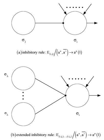
Figure 1. (a) inhibitory rule and (b) extended inhibitory rule.

A neuron may have multiple inhibitory neurons. As shown in Figure 1b, neuron ${\mathrm{\sigma }}_{\mathrm{i}}$ has z inhibitory neurons ${\mathrm{\sigma }}_{{\mathrm{j}}_1},\dots ,\mathrm{\sigma }{}_{{\mathrm{j}}_{\mathrm{z}}}$. At this time, the form of inhibitory rules is ${\mathrm{E}}_{\left(\mathrm{i},{\mathrm{j}}_1\right),\dots ,\left(\mathrm{i},{\mathrm{j}}_{\mathrm{z}}\right)}/\left({\mathrm{a}}^{\mathrm{u}},\overline{{\mathrm{a}}^{\mathrm{\tau }}}\right)\to {\mathrm{a}}^{\mathrm{p}}\left(1\right)$, which is called an extended inhibitory rule. The firing condition of the extended inhibitory rule is ${\mathrm{u}}_{\mathrm{i}}(\mathrm{t})\ge {\mathrm{\tau }}_{\mathrm{i}}(\mathrm{t}),{\mathrm{u}}_{\mathrm{i}}(\mathrm{t})\ge \mathrm{u},{\mathrm{\tau }}_{\mathrm{i}}\left(\mathrm{t}\right)\ge \mathrm{\tau }$, and ${\mathrm{u}}_{{\mathrm{j}}_1}\left(\mathrm{t}\right)={\mathrm{\tau }}_{\mathrm{i}}\left(\mathrm{t}\right)\wedge \dots \wedge {\mathrm{u}}_{{\mathrm{j}}_{\mathrm{z}}}\left(\mathrm{t}\right)={\mathrm{\tau }}_{\mathrm{i}}\left(\mathrm{t}\right)$.

If neuron ${\mathrm{\sigma }}_{\mathrm{i}}$ meets firing conditions during calculation, then one of the rules in ${\mathrm{R}}_{\mathrm{i}}$ must be used. If two rules ${\mathrm{E}}_{\mathrm{i}}/\left({\mathrm{a}}^{\mathrm{u}},{\mathrm{a}}^{\mathrm{\tau }}\right)\to {\mathrm{a}}^{\mathrm{p}}(\mathrm{l})$ and ${\mathrm{E}}_{{\mathrm{i}}^{’}}/\left({\mathrm{a}}^{{\mathrm{u}}^{‘}},{\mathrm{a}}^{{\mathrm{\tau }}^{’}}\right)\to {\mathrm{a}}^{{\mathrm{p}}^{‘}}(\mathrm{l})$ in neuro n ${\mathrm{\sigma }}_{\mathrm{i}}$ can be applied to configuration ${\mathrm{C}}_{\mathrm{t}}$ at the same time, only one of them can be applied. According to the maximum spikes consumption strategy of DTNP-MCIR systems, when $\mathrm{u}+\mathrm{\tau }-\mathrm{p}-{\mathrm{n}}_1>{\mathrm{u}}^{\prime }+{\mathrm{\tau }}^{\prime }-{\mathrm{p}}^{\prime }-{\mathrm{n}}_2$, the rule ${\mathrm{E}}_{\mathrm{i}}/\left({\mathrm{a}}^{\mathrm{u}},{\mathrm{a}}^{\mathrm{\tau }}\right)\to {\mathrm{a}}^{\mathrm{p}}(\mathrm{l})$ is applied, otherwise, the rule ${\mathrm{E}}_{{\mathrm{i}}^{’}}/\left({\mathrm{a}}^{{\mathrm{u}}^{‘}},{\mathrm{a}}^{{\mathrm{\tau }}^{’}}\right)\to {\mathrm{a}}^{{\mathrm{p}}^{‘}}(\mathrm{l})$ is applied, when $\mathrm{u}+\mathrm{\tau }-\mathrm{p}-{\mathrm{n}}_1={\mathrm{u}}^{\prime }+{\mathrm{\tau }}^{\prime }-{\mathrm{p}}^{\prime }-{\mathrm{n}}_2$, one of them will be non-deterministically selected. Note that this strategy is also effective for forgetting rules. For example, two rules ${\mathrm{E}}_1/\left({\mathrm{a}}^2,\mathrm{a}\right)\to \mathrm{\lambda }$ and ${\mathrm{E}}_2/\left(\mathrm{a},\mathrm{a}\right)\to \mathrm{a}(\mathrm{l})$ both satisfy firing conditions at time t, since the firing of forgetting rule ${\mathrm{E}}_1/\left({\mathrm{a}}^2,\mathrm{a}\right)\to \mathrm{\lambda }$ consumes three spikes, however, the spiking rule ${\mathrm{E}}_2/\left(\mathrm{a},\mathrm{a}\right)\to \mathrm{a}(\mathrm{l})$ only consumes one spike, then the forgetting rule will be chose and applied.

We assume that a transition step is from one configuration to another. A sequence of transitions from the initial configuration is defined as a calculation. For a configuration ${\mathrm{C}}_{\mathrm{t}}$, if no rules in the system can be applied, the system calculation halts. Any calculation corresponds to a binary sequence, write 1 when the output neuron ${\mathrm{\sigma }}_{\mathrm{o}\mathrm{u}\mathrm{t}}$ emit a spike to the environment, otherwise write 0. Therefore, the calculation result is defined as the time interval between the first two spikes emitted by the output neuron ${\mathrm{\sigma }}_{\mathrm{o}\mathrm{u}\mathrm{t}}$. ${\mathrm{N}}_2(\mathrm{\Pi })$ represents a set of numbers calculated by system $\mathrm{\Pi }$. ${\mathrm{N}}_2\mathrm{D}\mathrm{T}\mathrm{N}\mathrm{P}-\mathrm{M}\mathrm{C}\mathrm{I}{\mathrm{R}}_{\mathrm{m}}^{\mathrm{n}}$ denotes the families of all sets ${\mathrm{N}}_2(\mathrm{\Pi })$ accepted by DTNP-MCIR systems having at most m neurons and at most n rules in each neuron. When m or n is not restricted, the symbol “*” is usually used instead. System $\mathrm{\Pi }$ can be used as a accepting device, at this time, the input neuron receives spikes from the environment, but the output neuron is removed from the system. The system imports spikes train from the environment, then stores the number n in the form of 2n spikes. When the system calculation halts, n is the number to be accepted by it. ${\mathrm{N}}_{\mathrm{a}\mathrm{c}\mathrm{c}}(\mathrm{\Pi })$ represents a set of numbers accepted by the system, ${\mathrm{N}}_{\mathrm{a}\mathrm{c}\mathrm{c}}\mathrm{D}\mathrm{T}\mathrm{N}\mathrm{P}-\mathrm{M}\mathrm{C}\mathrm{I}{\mathrm{R}}_{\mathrm{m}}^{\mathrm{n}}$ denotes the families of all sets ${\mathrm{N}}_{\mathrm{a}\mathrm{c}\mathrm{c}}(\mathrm{\Pi })$ accepted by DTNP-MCIR systems having at most m neurons and at most n rules in each neuron.

2.2. Illustrative Example

In order to clearly understand the working mechanism of DTNP-MCIR systems, we give an example that can generate a finite spike train, as shown in Figure 2.

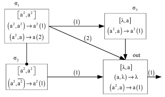
Figure 2. An illustrative example.

We assume that a DTNP-MCIR system $\mathrm{\Pi }$ consists of four neurons ${\mathrm{\sigma }}_1,{\mathrm{\sigma }}_2,{\mathrm{\sigma }}_3,\mathrm{out}$. Initially, the feeding input units of neuron ${\mathrm{\sigma }}_1$ and neuron ${\mathrm{\sigma }}_2$ each have two spikes, but there are no spikes in neuron ${\mathrm{\sigma }}_3$ and out, that is ${\mathrm{u}}_1(0)=2,{\mathrm{u}}_2(0)=2,{\mathrm{u}}_3(0)=0,{\mathrm{u}}_{\mathrm{o}\mathrm{u}\mathrm{t}}(0)=0$. The number of spikes in the initial dynamic threshold unit of the four neurons is ${\mathrm{\tau }}_1(0)=2,{\mathrm{\tau }}_2(0)=2,{\mathrm{\tau }}_3(0)=1,{\mathrm{\tau }}_{\mathrm{out}}(0)=1$ respectively. Therefore, the initial configuration ${\mathrm{C}}_0=\left(\left[2,2\right],\left[2,2\right]\left[0,1\right],\left[0,1\right]\right)$.

At time 1, since ${\mathrm{u}}_1(0)=2\ge {\mathrm{\tau }}_1(0)=2$, rules $({\mathrm{a}}^2,{\mathrm{a}}^2)\to {\mathrm{a}}^2(1)(\mathrm{u}=\mathrm{\tau }=\mathrm{p}=2)$ and $({\mathrm{a}}^2,\mathrm{a})\to \mathrm{a}(2)({\mathrm{u}}^{\prime }=2,{\mathrm{\tau }}^{\prime }={\mathrm{p}}^{\prime }=1)$ can be applied in neuron ${\mathrm{\sigma }}_1$, and since the number of spikes consumption for both rules is $\mathrm{u}+\mathrm{\tau }-\mathrm{p}={\mathrm{u}}^{\prime }+{\mathrm{\tau }}^{\prime }-{\mathrm{p}}^{\prime }=2$, one of them will be selected non-deterministically. Therefore, there are the following two cases:

(1)

Case 1: if rule $({\mathrm{a}}^2,{\mathrm{a}}^2)\to {\mathrm{a}}^2(1)$ is applied in neuron ${\mathrm{\sigma }}_1$ at time 1, then neuron ${\mathrm{\sigma }}_1$ will consume two spikes in the feeding input unit and sends two spikes to the neuron ${\mathrm{\sigma }}_3$ through channel (1). Neuron ${\mathrm{\sigma }}_1$ is the inhibitory neuron of neuron ${\mathrm{\sigma }}_2$, since ${\mathrm{u}}_2(0)=2\ge {\mathrm{\tau }}_2(0)=2$ and ${\mathrm{u}}_1(0)={\mathrm{\tau }}_2(0)$, rule $({\mathrm{a}}^2,\overline{{\mathrm{a}}^2})\to {\mathrm{a}}^2(1)$ reaches the firing condition in neuron ${\mathrm{\sigma }}_2$, so neuron ${\mathrm{\sigma }}_2$ consumes two spikes in the feeding input unit and sends two spikes to the neuron out via channel (1) at time 1. Therefore, ${\mathrm{C}}_1=\left(\left[0,2\right],\left[0,2\right]\left[2,1\right],\left[2,1\right]\right)$. At time 2, since ${\mathrm{u}}_{\mathrm{o}\mathrm{u}\mathrm{t}}(1)=2\ge {\mathrm{\tau }}_{\mathrm{o}\mathrm{u}\mathrm{t}}(1)=1$, both rule $\left({\mathrm{a}}^2,\mathrm{a}\right)\to \mathrm{a}(1)$ and rule $(\mathrm{a},\mathrm{\lambda })\to \mathrm{\lambda }(2)$ in neuron out can be applied. However, according to the maximum spike consumption strategy, rule $\left({\mathrm{a}}^2,\mathrm{a}\right)\to \mathrm{a}(1)$ will be applied and sends one spike to the environment through channel (1). Further, since ${\mathrm{u}}_3(1)=2\ge {\mathrm{\tau }}_3(1)=1$, rule $({\mathrm{a}}^2,\mathrm{a})\to \mathrm{a}(1)$ is enable in neuron ${\mathrm{\sigma }}_3$ and consumes two spikes in the feeding input unit and sends two spike to neuron out. Thus ${\mathrm{C}}_2=\left(\left[0,2\right],\left[0,2\right]\left[0,2\right],\left[2,1\right]\right)$. At time 3, since ${\mathrm{u}}_{\mathrm{o}\mathrm{u}\mathrm{t}}(2)=2\ge {\mathrm{\tau }}_{\mathrm{o}\mathrm{u}\mathrm{t}}(2)=1$, rule $({\mathrm{a}}^2,\mathrm{a})\to \mathrm{a}(1)$ fires again and sends one spike to the environment. The system $\mathrm{\Pi }$ halts. Therefore, the spike train generated by this system is “011”.

(2)

Case 2: if rule $({\mathrm{a}}^2,\mathrm{a})\to {\mathrm{a}}^2(2)$ is applied in neuron ${\mathrm{\sigma }}_1$ at time 1, then neuron ${\mathrm{\sigma }}_1$ consumes two spikes in the feeding input unit and sends one spikes to the neuron out through channel (2). Because the state of system $\mathrm{\Pi }$ is the same as that in case 1 at time 1, neuron ${\mathrm{\sigma }}_2$ consumes two spikes in the feeding input unit and sends two spikes to the neuron out through channel (1).So ${\mathrm{C}}_1=\left(\left[0,3\right],\left[0,2\right]\left[0,1\right],\left[3,1\right]\right)$. At time 2, since ${\mathrm{u}}_{\mathrm{o}\mathrm{u}\mathrm{t}}(1)=3\ge {\mathrm{\tau }}_{\mathrm{o}\mathrm{u}\mathrm{t}}(1)=1$, also according to the maximum spike consumption strategy, neuron out fires by the rule $({\mathrm{a}}^2,\mathrm{a})\to \mathrm{a}(1)$ and sends one spike to the environment through channel (1). The configuration of System $\mathrm{\Pi }$ at this time is ${\mathrm{C}}_1=\left(\left[0,3\right],\left[0,2\right]\left[0,1\right],\left[1,1\right]\right)$. At time 3, since ${\mathrm{u}}_{\mathrm{o}\mathrm{u}\mathrm{t}}(2)=1\ge {\mathrm{\tau }}_{\mathrm{o}\mathrm{u}\mathrm{t}}(2)=1$, rule $(\mathrm{a},\mathrm{\lambda })\to \mathrm{\lambda }$ is applied and removes one spike in feeding input unit and the system $\mathrm{\Pi }$ halts. Therefore, the spike train generated is “010”.

3. Turing Universality of DTNP-MCIR Systems as Number-Generating/Accepting Device

In this section, we will explain the working mechanism of DTNP-MCIR systems as the number generating and number accepting mode. DTNP-MCIR systems proves its computational completeness by simulating register machines. More specifically, DTNP-MCIR systems can generate/accept all recursively enumerable sets of numbers (their family is called NRE).

A register machine can be defined as $\mathrm{M}=(\mathrm{m},\mathrm{H},{\mathrm{l}}_0,{\mathrm{l}}_{\mathrm{h}}\mathrm{I})$, where m is the number of registers, H indicates the set of instruction labels, ${\mathrm{l}}_0$ corresponds to the start label, ${\mathrm{l}}_{\mathrm{h}}$ corresponds to the halt label, I denotes the set of instructions. Each instruction in I corresponds to a label in H, the instructions in I have the following three forms:

(1)

${\mathrm{l}}_{\mathrm{i}}:(\mathrm{A}\mathrm{D}\mathrm{D}(\mathrm{r}),{\mathrm{l}}_{\mathrm{j}},{\mathrm{l}}_{\mathrm{k}})$ (add 1 to register r and then move non-deterministically to one of the instructions with labels ${\mathrm{l}}_{\mathrm{j}}$, ${\mathrm{l}}_{\mathrm{k}}$ ).

(2)

${\mathrm{l}}_{\mathrm{j}}:(\mathrm{S}\mathrm{U}\mathrm{B}(\mathrm{r}),{\mathrm{l}}_{\mathrm{j}},{\mathrm{l}}_{\mathrm{k}})$ (if register r is non-zero, then subtract 1 from it, and go to the instruction with label ${\mathrm{l}}_{\mathrm{j}}$; otherwise go to the instruction with label ${\mathrm{l}}_{\mathrm{k}}$).

(3)

${\mathrm{l}}_{\mathrm{h}}:\mathrm{H}\mathrm{A}\mathrm{L}\mathrm{T}$ (halting instruction).

3.1. DTNP-MCIR Systems as Number Generating Devices

Initially, every register in the register machine M is empty. The register machine can calculate the number n in the generation mode. It first starts with instruction ${\mathrm{l}}_0$, and then applies a series of instructions until it reaches the halting instruction ${\mathrm{l}}_{\mathrm{h}}$. Finally, the number stored in the first register is the result calculated by the register machine. Usually the family NRE can be characterized by the register machine.

Theorem 1.

$N_{2}SN{P}_{*}^2=NRE$.

Proof. 

As we all know, ${\mathrm{N}}_2\mathrm{S}\mathrm{N}{\mathrm{P}}_{*}^2\subseteq \mathrm{NRE}$. So we only need to prove $\mathrm{NRE}\subseteq {\mathrm{N}}_2\mathrm{S}\mathrm{N}{\mathrm{P}}_{*}^2$ we consider a register machine $\mathrm{M}=(\mathrm{m},\mathrm{H},{\mathrm{l}}_0,{\mathrm{l}}_{\mathrm{h}}\mathrm{I})$ that works in generation mode, assuming that all registers except register 1 are empty, and register 1 never decrements during the calculation. □

We designed a DTNP-MCIR system ${\mathrm{\Pi }}_1$ to simulate the register machine working in generating mode. The system ${\mathrm{\Pi }}_1$ includes three modules: ADD module, SUB module, and FIN module. ADD module and SUB module used to simulate the ADD instruction and the SUB instruction respectively, and FIN module deals with the calculation results of the system ${\mathrm{\Pi }}_1$.

We stipulate that each register r of register machine M corresponds to a neuron ${\mathrm{\sigma }}_{\mathrm{r}}$, note that there are no rules in neuron ${\mathrm{\sigma }}_{\mathrm{r}}$,numbers can be encoded in neuron ${\mathrm{\sigma }}_{\mathrm{r}}$. If the number stored in the register r is $\mathrm{n}\ge 0$, then neuron ${\mathrm{\sigma }}_{\mathrm{r}}$ contains 2n spikes. Each instruction l corresponds to a neuron ${\mathrm{\sigma }}_{\mathrm{l}}$, and some auxiliary neurons are introduced into models. Assume that there are no spikes in the feeding input unit of all auxiliary neurons, but neuron ${\mathrm{\sigma }}_{\mathrm{l}\mathrm{i}}$ receives two spikes at the beginning. Each neuron has an initial threshold for the initial threshold unit: (i) the initial threshold of each instruction neuron ${\mathrm{\sigma }}_{\mathrm{l}}$ is ${\mathrm{a}}^2$; (ii) each register neuron ${\mathrm{\sigma }}_{\mathrm{r}}$ contains an initial threshold of a; (iii) the initial threshold of other neurons is uncertain. Because neuron ${\mathrm{\sigma }}_{\mathrm{l}\mathrm{i}}$ gets two spikes, the system ${\mathrm{\Pi }}_1$ begin to simulate the instruction n ${\mathrm{l}}_{\mathrm{i}}=\left(\mathrm{O}\mathrm{P}(\mathrm{r}),{\mathrm{l}}_{\mathrm{j}},{\mathrm{l}}_{\mathrm{k}}\right)$ (OP represents one of ADD or SUB operations). Starting from the activated neuron ${\mathrm{\sigma }}_{\mathrm{l}\mathrm{i}}$, the simulation deals with neuron ${\mathrm{\sigma }}_{\mathrm{r}}$ according to OP, and then two spikes are introduced to one of the neurons ${\mathrm{\sigma }}_{\mathrm{l}\mathrm{j}}$ and ${\mathrm{\sigma }}_{\mathrm{l}\mathrm{k}}$. The simulation will continue until the neuron ${\mathrm{\sigma }}_{\mathrm{l}\mathrm{h}}$ fires, indicating that the simulation is completed [30]. In the calculation process, the spikes are sent to the environment twice by neuron ${\mathrm{\sigma }}_{\mathrm{o}\mathrm{u}\mathrm{t}}$ at times ${\mathrm{t}}_1$ and ${\mathrm{t}}_2$ respectively, the calculation result is defined as the interval of ${\mathrm{t}}_2-{\mathrm{t}}_1$ that is also the number contained in register1.

In order to verify that the system ${\mathrm{\Pi }}_1$ can indeed simulate the register machine M correctly, we will explain how the ADD or SUB module simulates the ADD or SUB instruction, and how the FIN module outputs the calculation results.

(1)

ADD module (shown in Figure 3)—simulating an ADD instruction ${\mathrm{l}}_{\mathrm{i}}:(\mathrm{A}\mathrm{D}\mathrm{D}(\mathrm{r}),{\mathrm{l}}_{\mathrm{j}},{\mathrm{l}}_{\mathrm{k}})$

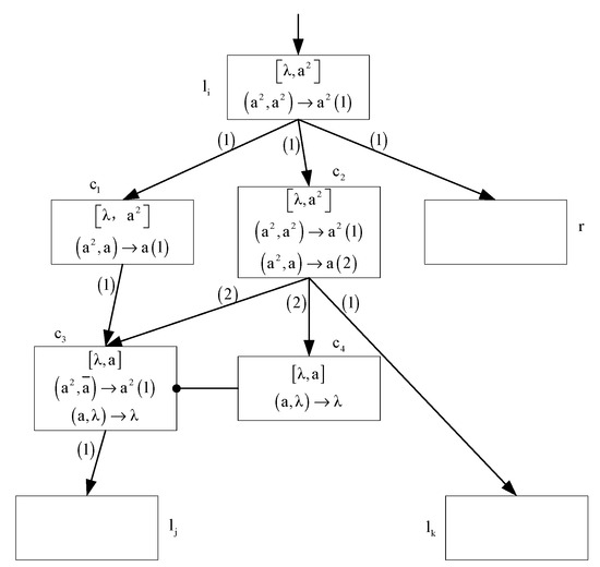Figure 3. Module ADD simulating the ADD instruction ${\mathrm{l}}_{\mathrm{i}}:\left(\mathrm{A}\mathrm{D}\mathrm{D}\left(\mathrm{r}\right),{\mathrm{l}}_{\mathrm{j}},{\mathrm{l}}_{\mathrm{k}}\right)$.

The system ${\mathrm{\Pi }}_1$ starts from ADD instruction ${\mathrm{l}}_0$. Suppose an ADD instruction ${\mathrm{l}}_{\mathrm{i}}:(\mathrm{A}\mathrm{D}\mathrm{D}(\mathrm{r}),{\mathrm{l}}_{\mathrm{j}},{\mathrm{l}}_{\mathrm{k}})$ is simulated at time t. At this time, neuron ${\mathrm{\sigma }}_{{\mathrm{l}}_{\mathrm{i}}}$ contains two spikes and the configuration of module ADD is ${\mathrm{C}}_{\mathrm{t}}=\left(\left[{\mathrm{u}}_1,{\mathrm{\tau }}_1\right],\left[{\mathrm{u}}_2,{\mathrm{\tau }}_2\right],\dots ,\left[{\mathrm{u}}_7,{\mathrm{\tau }}_7\right],\right)$, which involves 7 neurons ${\mathrm{\sigma }}_{{\mathrm{l}}_{\mathrm{i}}},{\mathrm{\sigma }}_{{\mathrm{c}}_1},{\mathrm{\sigma }}_{{\mathrm{c}}_2},{\mathrm{\sigma }}_{{\mathrm{c}}_3},{\mathrm{\sigma }}_{{\mathrm{c}}_4},{\mathrm{\sigma }}_{{\mathrm{l}}_{\mathrm{j}}},{\mathrm{\sigma }}_{{\mathrm{l}}_{\mathrm{k}}}$ respectively. Thus, ${\mathrm{C}}_{\mathrm{t}}=\left(\left[2,2\right],\left[0,2\right],\left[0,2\right],\left[0,1\right],\left[0,1\right],\left[0,2\right],\left[0,2\right]\right)$. Since ${\mathrm{u}}_{\mathrm{l}\mathrm{i}}(\mathrm{t})=2\ge {\mathrm{\tau }}_{\mathrm{l}\mathrm{i}}(\mathrm{t})=2$, rule $\left({\mathrm{a}}^2,{\mathrm{a}}^2\right)\to {\mathrm{a}}^2(1)$ is applied in neuron ${\mathrm{\sigma }}_{{\mathrm{l}}_{\mathrm{i}}}$,then two spikes are sent to neurons ${\mathrm{\sigma }}_{{\mathrm{c}}_1},{\mathrm{\sigma }}_{{\mathrm{c}}_2},{\mathrm{\sigma }}_{\mathrm{r}}$ via channel (1). Because neuron ${\mathrm{\sigma }}_{\mathrm{r}}$ receives two spikes, register r increases by one. Thus, ${\mathrm{C}}_{\mathrm{t}+1}=\left(\left[0,2\right],\left[2,2\right],\left[2,2\right],\left[0,1\right],\left[0,1\right],\left[0,2\right],\left[0,2\right]\right)$.

At time t + 1, both feeding input unit and dynamic threshold unit of neuron ${\mathrm{\sigma }}_{{\mathrm{c}}_1}$ and neuron ${\mathrm{\sigma }}_{{\mathrm{c}}_2}$ contain two spikes, so they fire. Rule $\left({\mathrm{a}}^2,\mathrm{a}\right)\to \mathrm{a}(1)$ in neuron ${\mathrm{\sigma }}_{{\mathrm{c}}_1}$ is applied and send one spike to neuron ${\mathrm{\sigma }}_{{\mathrm{c}}_3}$. For neuron ${\mathrm{\sigma }}_{{\mathrm{c}}_2}$, rules $\left({\mathrm{a}}^2,{\mathrm{a}}^2\right)\to {\mathrm{a}}^2(1)$ and $\left({\mathrm{a}}^2,\mathrm{a}\right)\to \mathrm{a}(2)$ both satisfy the firing condition, and both consume an equal number of spikes, so one of them will be selected non-deterministically. We consider the following two cases:

(i)

At time t + 1, if rule $\left({\mathrm{a}}^2,{\mathrm{a}}^2\right)\to {\mathrm{a}}^2(1)$ is applied, neuron ${\mathrm{\sigma }}_{{\mathrm{c}}_2}$ sends two spikes to neuron ${\mathrm{\sigma }}_{{\mathrm{l}}_{\mathrm{k}}}$ via channel (1). Then neuron ${\mathrm{\sigma }}_{{\mathrm{l}}_{\mathrm{k}}}$ receives two spikes, system ${\mathrm{\Pi }}_1$ starts to simulate instruction ${\mathrm{l}}_{\mathrm{k}}$. Therefore ${\mathrm{C}}_{\mathrm{t}+2}=\left(\left[0,2\right],\left[0,2\right],\left[0,2\right],\left[1,1\right],\left[0,1\right],\left[0,2\right],\left[2,2\right]\right)$. At time t + 3, since ${\mathrm{u}}_{{\mathrm{c}}_3}\left(\mathrm{t}+2\right)=1\ge {\mathrm{\tau }}_{{\mathrm{c}}_3}\left(\mathrm{t}+2\right)=1,$ the rule $\left(\mathrm{a},\mathrm{\lambda }\right)\to \mathrm{\lambda }$ of neuron ${\mathrm{\sigma }}_{{\mathrm{c}}_3}$ is enabled and removes the only spike in the feeding input unit.

(ii)

At time t + 1, if rule $\left({\mathrm{a}}^2,\mathrm{a}\right)\to \mathrm{a}(2)$ is applied, neuron ${\mathrm{\sigma }}_{{\mathrm{c}}_2}$ sends one spike to neurons ${\mathrm{\sigma }}_{{\mathrm{c}}_3}$ and ${\mathrm{\sigma }}_{{\mathrm{c}}_4}$ via channel (2). Thus, ${\mathrm{C}}_{\mathrm{t}+2}=\left(\left[0,2\right],\left[0,2\right],\left[0,2\right],\left[2,1\right],\left[1,1\right],\left[0,2\right],\left[0,2\right]\right)$. Note that neuron ${\mathrm{\sigma }}_{{\mathrm{c}}_4}$ is the inhibitory neuron of neuron ${\mathrm{\sigma }}_{{\mathrm{c}}_3}$, since ${\mathrm{u}}_{{\mathrm{c}}_4}\left(\mathrm{t}+2\right)={\mathrm{\tau }}_{{\mathrm{c}}_3}\left(\mathrm{t}+2\right)$, inhibitory rule $\left({\mathrm{a}}^2,\overline{\mathrm{a}}\right)\to {\mathrm{a}}^2(1)$ is enabled, neuro n ${\mathrm{\sigma }}_{{\mathrm{c}}_3}$ sends two spikes to neuron ${\mathrm{\sigma }}_{{\mathrm{l}}_{\mathrm{j}}}$. This means that the system ${\mathrm{\Pi }}_1$ starts to simulate instruction ${\mathrm{l}}_{\mathrm{j}}$. The configuration of ${\mathrm{\Pi }}_1$ at this time is ${\mathrm{C}}_{\mathrm{t}+3}=\left(\left[0,2\right],\left[0,2\right],\left[0,2\right],\left[0,1\right],\left[0,1\right],\left[2,2\right],\left[0,2\right]\right)$.

Therefore, ADD instructions can be correctly simulated by the ADD module. Since neuron ${\mathrm{\sigma }}_{{\mathrm{l}}_{\mathrm{i}}}$ has two spikes, two spikes are added to neuron ${\mathrm{\sigma }}_{\mathrm{r}}$, and then neuron ${\mathrm{\sigma }}_{{\mathrm{l}}_{\mathrm{j}}}$ and ${\mathrm{\sigma }}_{{\mathrm{l}}_{\mathrm{k}}}$ are selected non-deterministically.

(2)

SUB module (shown in Figure 4)—simulating a SUB instruction ${\mathrm{l}}_{\mathrm{j}}:(\mathrm{S}\mathrm{U}\mathrm{B}(\mathrm{r}),{\mathrm{l}}_{\mathrm{j}},{\mathrm{l}}_{\mathrm{k}})$.

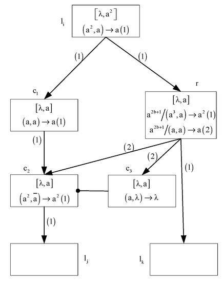Figure 4. Module SUB simulating a SUB instruction ${\mathrm{l}}_{\mathrm{j}}:(\mathrm{S}\mathrm{U}\mathrm{B}(\mathrm{r}),{\mathrm{l}}_{\mathrm{j}},{\mathrm{l}}_{\mathrm{k}})$.

Suppose that the system ${\mathrm{\Pi }}_1$ starts to simulate the SUB instruction ${\mathrm{l}}_{\mathrm{j}}:(\mathrm{S}\mathrm{U}\mathrm{B}(\mathrm{r}),{\mathrm{l}}_{\mathrm{j}},{\mathrm{l}}_{\mathrm{k}})$ at time t, and neuron ${\mathrm{\sigma }}_{{\mathrm{l}}_{\mathrm{i}}}$ contains two spikes at the same time. The configuration of module SUB is ${\mathrm{C}}_{\mathrm{t}}{}^{\prime }=\left(\left[{\mathrm{u}}_1,{\mathrm{\tau }}_1\right],\left[{\mathrm{u}}_2,{\mathrm{\tau }}_2\right],\dots ,\left[{\mathrm{u}}_7,{\mathrm{\tau }}_7\right],\right)$, which involves 7 neurons ${\mathrm{\sigma }}_{{\mathrm{l}}_{\mathrm{i}}},{\mathrm{\sigma }}_{\mathrm{r}},{\mathrm{\sigma }}_{{\mathrm{c}}_1},{\mathrm{\sigma }}_{{\mathrm{c}}_2},{\mathrm{\sigma }}_{{\mathrm{c}}_3},{\mathrm{\sigma }}_{{\mathrm{l}}_{\mathrm{j}}},{\mathrm{\sigma }}_{{\mathrm{l}}_{\mathrm{k}}}$ respectively. Thus, ${\mathrm{C}}_{\mathrm{t}}{}^{\prime }=\left(\left[2,2\right],\left[2\mathrm{n},1\right],\left[0,1\right],\left[0,1\right],\left[0,1\right],\left[0,2\right],\left[0,2\right]\right)$. Since ${\mathrm{u}}_{{\mathrm{l}}_{\mathrm{i}}}(\mathrm{t})=2\ge {\mathrm{\tau }}_{{\mathrm{l}}_{\mathrm{i}}}(\mathrm{t})=2$, neuron ${\mathrm{\sigma }}_{{\mathrm{l}}_{\mathrm{i}}}$ fires and sends a spike to neuron ${\mathrm{\sigma }}_{\mathrm{r}}$ and ${\mathrm{\sigma }}_{{\mathrm{c}}_1}$ via channel (1). Therefore ${\mathrm{C}}_{\mathrm{t}+1}{}^{\prime }=\left(\left[0,2\right],\left[2\mathrm{n}+1,1\right],\left[1,1\right],\left[0,1\right],\left[0,1\right],\left[0,2\right],\left[0,2\right]\right)$. Based on the number of spikes in neuron ${\mathrm{\sigma }}_{\mathrm{r}}$, there are two cases:

(i)

If feeding input unit of neuron ${\mathrm{\sigma }}_{\mathrm{r}}$ contains $2\mathrm{n}\ge 0$ spikes at time t, then at time t + 1, neuron ${\mathrm{\sigma }}_{\mathrm{r}}$ contains $2\mathrm{n}+1\ge 3$ spikes. At time t + 2, rule ${\mathrm{a}}^{2\mathrm{b}+1}/\left({\mathrm{a}}^3,\mathrm{a}\right)\to {\mathrm{a}}^2(1)$ will be enabled and neuron ${\mathrm{\sigma }}_{\mathrm{r}}$ will send two spikes to neurons ${\mathrm{\sigma }}_{{\mathrm{l}}_{\mathrm{k}}}$ via channel (1). This indicates that system ${\mathrm{\Pi }}_1$ starts to simulate the instruction ${\mathrm{l}}_{\mathrm{k}}$ of register machine M. In addition, rule $\left(\mathrm{a},\mathrm{a}\right)\to \mathrm{a}(1)$ satisfies firing condition, neuron ${\mathrm{\sigma }}_{{\mathrm{c}}_1}$ sends a spike to neuron ${\mathrm{\sigma }}_{{\mathrm{c}}_2}$. Thus ${\mathrm{C}}_{\mathrm{t}+2}{}^{\prime }=\left(\left[0,2\right],\left[2\mathrm{n}-2,1\right],\left[0,1\right],\left[1,1\right],\left[0,1\right],\left[0,2\right],\left[2,2\right]\right)$. At time t+3, the forgetting rule $\left(\mathrm{a},\mathrm{\lambda }\right)\to \mathrm{\lambda }$ of neuron ${\mathrm{\sigma }}_{{\mathrm{c}}_2}$ is enabled and removes the only spike in the feeding input unit. Therefore, ${\mathrm{C}}_{\mathrm{t}+3}{}^{\prime }=\left(\left[0,2\right],\left[2\mathrm{n}-2,1\right],\left[0,1\right],\left[0,1\right],\left[0,1\right],\left[0,2\right],\left[2,2\right]\right)$.

(ii)

If feeding input unit of neuron ${\mathrm{\sigma }}_{\mathrm{r}}$ does not contain spikes at time t, then at time t + 1, neuron ${\mathrm{\sigma }}_{\mathrm{r}}$ contains only one spike. At time t + 2, rule ${\mathrm{a}}^{2\mathrm{b}+1}/\left(\mathrm{a},\mathrm{a}\right)\to \mathrm{a}(1)$ will be applied and neuron ${\mathrm{\sigma }}_{\mathrm{r}}$ will transmit one spike to neurons ${\mathrm{\sigma }}_{{\mathrm{c}}_2}$ and ${\mathrm{\sigma }}_{{\mathrm{c}}_3}$ via channel (2). At the same time neuron ${\mathrm{\sigma }}_{{\mathrm{c}}_1}$ also transmits a spike to neuron ${\mathrm{\sigma }}_{{\mathrm{c}}_2}$. So ${\mathrm{C}}_{\mathrm{t}+2}{}^{\prime }=\left(\left[0,2\right],\left[0,1\right],\left[0,1\right],\left[2,1\right],\left[1,1\right],\left[0,2\right],\left[0,2\right]\right)$. Note that neuron ${\mathrm{\sigma }}_{{\mathrm{c}}_3}$ is the inhibitory neuron of neuron ${\mathrm{\sigma }}_{{\mathrm{c}}_2}$. At time t + 3, the forgetting rule $\left(\mathrm{a},\mathrm{\lambda }\right)\to \mathrm{\lambda }$ of neuron ${\mathrm{\sigma }}_{{\mathrm{c}}_3}$ is enabled and removes the only spike in the feeding input unit. Moreover, since ${\mathrm{u}}_{{\mathrm{c}}_3}\left(\mathrm{t}+2\right)={\mathrm{\tau }}_{{\mathrm{c}}_2}\left(\mathrm{t}+2\right)$, rule $\left({\mathrm{a}}^2,\overline{\mathrm{a}}\right)\to {\mathrm{a}}^2(1)$ is applied, neuron ${\mathrm{\sigma }}_{{\mathrm{c}}_2}$ sends two spikes to neuron ${\mathrm{\sigma }}_{{\mathrm{l}}_{\mathrm{j}}}$. This means that the system ${\mathrm{\Pi }}_1$ starts to simulate instruction ${\mathrm{l}}_{\mathrm{j}}$. Thus, ${\mathrm{C}}_{\mathrm{t}+2}{}^{\prime }=\left(\left[0,2\right],\left[0,1\right],\left[0,1\right],\left[0,2\right],\left[0,1\right],\left[2,2\right],\left[0,2\right]\right)$.

It can be seen from the above description that the SUB instruction can be correctly simulated by the SUB module. The system ${\mathrm{\Pi }}_1$ starts with neuron ${\mathrm{\sigma }}_{{\mathrm{l}}_{\mathrm{i}}}$ contains two spikes, then determine whether neuron ${\mathrm{\sigma }}_{{\mathrm{l}}_{\mathrm{k}}}$ or ${\mathrm{\sigma }}_{{\mathrm{l}}_{\mathrm{j}}}$ receives two spikes according to whether neuron ${\mathrm{\sigma }}_{\mathrm{r}}$ contains spikes.

(3)

Module FIN (shown in Figure 5)—outputting the result of computation

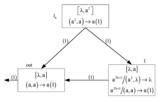Figure 5. FIN module.

We assume that neuron ${\mathrm{\sigma }}_1$ contains 2n spikes. Since neuron ${\mathrm{\sigma }}_{{\mathrm{l}}_{\mathrm{h}}}$ has two spikes at time t, it means register machine M halts, the rule $\left({\mathrm{a}}^2,\mathrm{a}\right)\to \mathrm{a}(1)$ is enabled and sends a spike to neurons ${\mathrm{\sigma }}_1$ and ${\mathrm{\sigma }}_{\mathrm{o}\mathrm{u}\mathrm{t}}$. Therefore, the number of spikes in neuron ${\mathrm{\sigma }}_1$ becomes an odd number. At time t + 1, rule $\left(\mathrm{a},\mathrm{a}\right)\to \mathrm{a}(1)$ in neuron ${\mathrm{\sigma }}_{\mathrm{o}\mathrm{u}\mathrm{t}}$ is enabled and sends the first spike to the environment. Moreover, both rule ${\mathrm{a}}^{2\mathrm{b}+1}/\left({\mathrm{a}}^2,\mathrm{\lambda }\right)\to \mathrm{\lambda }$ and rule ${\mathrm{a}}^{2\mathrm{b}+1}/\left(\mathrm{a},\mathrm{a}\right)\to \mathrm{a}(1)$ can be applied in neuron ${\mathrm{\sigma }}_1$. However, according to neuron’s maximum spike consumption strategy, forgetting rule ${\mathrm{a}}^{2\mathrm{b}+1}/\left({\mathrm{a}}^2,\mathrm{\lambda }\right)\to \mathrm{\lambda }$ is applied first and two spikes are eliminated. This process will repeat until there is only a spike in neuron ${\mathrm{\sigma }}_1$. At time $\mathrm{t}+\mathrm{n}$, neuron ${\mathrm{\sigma }}_1$ contains only a spike. Thus, the rule ${\mathrm{a}}^{2\mathrm{b}+1}/\left(\mathrm{a},\mathrm{a}\right)\to \mathrm{a}(1)$ is applied and transmits a spike to neuron ${\mathrm{\sigma }}_{\mathrm{o}\mathrm{u}\mathrm{t}}$. At time $\mathrm{t}+\mathrm{n}+1$, rule $\left(\mathrm{a},\mathrm{a}\right)\to \mathrm{a}(1)$ in neuron ${\mathrm{\sigma }}_{\mathrm{o}\mathrm{u}\mathrm{t}}$ is enabled and sends the second spike to the environment. The time interval between two spikes being transmitted to the environment is $\mathrm{n}=\left(\mathrm{t}+1\right)-\left(\mathrm{t}+\mathrm{n}+1\right)$, which is the number in register ${\mathrm{\sigma }}_1$ when the register machine halts.

According to the above description, it can be found that the system ${\mathrm{\Pi }}_1$ can correctly simulate register machine M working in generating module. Therefore, Theorem 1 holds.

3.2. Turing Universality of Systems Working in the Accepting Mode

In the following, we will prove the universal of DTNP-MCIR systems as number accepting device.

Theorem 2.

$N_{acc}SN{P}_{*}^2=NRE$.

Proof. 

A DTNP-MCIR system ${\mathrm{\Pi }}_2$ is constructed to simulate a register machine $\mathrm{M}=\left(\mathrm{m},\mathrm{H},{\mathrm{l}}_0,{\mathrm{l}}_{\mathrm{h}},\mathrm{I}\right)$ working in the accepting mode. The setting of the initial threshold is the same as that used in the proof of Theorem 1 and initially any auxiliary neurons do not contain spikes. The proof is based on a modification to the proof of Theorem 1. System ${\mathrm{\Pi }}_2$ contains a deterministic ADD module, a SUB module, and an INPUT module. □

Figure 6 shows the input module where neuron ${\mathrm{\sigma }}_{\mathrm{i}\mathrm{n}}$ is used to read the spike train ${10}^{\mathrm{n}-1}1$ from the environment. The number accepted by system ${\mathrm{\Pi }}_2$ is the interval ( $\mathrm{n}=\left(\mathrm{n}+1\right)-1$ ) between two spikes in the spike train.

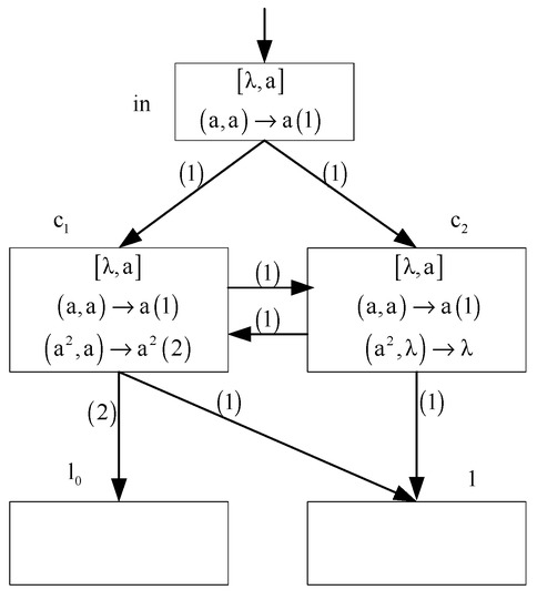
Figure 6. The INPUT module of ${\mathrm{\Pi }}_2$.

Suppose that neuron ${\mathrm{\sigma }}_{\mathrm{in}}$ imports the first spike from the environment at time t. Therefore, the initial configuration of System ${\mathrm{\Pi }}_2$ is ${\mathrm{C}}_{\mathrm{t}}=\left(\left[1,1\right],\left[0,1\right],\left[0,1\right],\left[0,2\right],\left[0,1\right]\right)$, which involves 5 neurons ${\mathrm{\sigma }}_{{\mathrm{l}}_{\mathrm{i}}},{\mathrm{\sigma }}_{{\mathrm{c}}_1},{\mathrm{\sigma }}_{{\mathrm{c}}_2},{\mathrm{\sigma }}_{{\mathrm{l}}_0},{\mathrm{\sigma }}_1$ respectively. Then rule $\left(\mathrm{a},\mathrm{a}\right)\to \mathrm{a}(1)$ in neuron ${\mathrm{\sigma }}_{\mathrm{in}}$ is enabled and sends a spike to neurons ${\mathrm{\sigma }}_{{\mathrm{c}}_1}$ and ${\mathrm{\sigma }}_{{\mathrm{c}}_2}$ via channel (1). Thus ${\mathrm{C}}_{\mathrm{t}+1}=\left(\left[0,1\right],\left[1,1\right],\left[1,1\right],\left[0,2\right],\left[0,1\right]\right)$. At time $\mathrm{t}+2$, the rule $\left(\mathrm{a},\mathrm{a}\right)\to \mathrm{a}(1)$ in neurons ${\mathrm{\sigma }}_{{\mathrm{c}}_1}$ and ${\mathrm{\sigma }}_{{\mathrm{c}}_2}$ is applied. From time t + 2 to the second spike is imported, neurons ${\mathrm{\sigma }}_{{\mathrm{c}}_1}$ and ${\mathrm{\sigma }}_{{\mathrm{c}}_2}$ both send a spike to neuron ${\mathrm{\sigma }}_1$ and exchange a spike with each other via channel (1). Thus neuron ${\mathrm{\sigma }}_1$ receives a total of 2n spikes from time t + 2 to time t + n + 1, which also indicates that the number contained in register 1 is n. At time t + n + 1, neuron ${\mathrm{\sigma }}_{\mathrm{i}\mathrm{n}}$ receives the second spike. The configuration of system ${\mathrm{\Pi }}_2$ at this time is ${\mathrm{C}}_{\mathrm{t}+\mathrm{n}+1}=\left(\left[1,1\right],\left[1,1\right],\left[1,1\right],\left[2\mathrm{n},2\right],\left[0,1\right]\right)$. At the next moment, the rule $\left(\mathrm{a},\mathrm{a}\right)\to \mathrm{a}(1)$ is enabled again and neuron ${\mathrm{\sigma }}_{\mathrm{in}}$ sends a spike to neurons ${\mathrm{\sigma }}_{{\mathrm{c}}_1}$ and ${\mathrm{\sigma }}_{{\mathrm{c}}_2}$. Thus, ${\mathrm{C}}_{\mathrm{t}+\mathrm{n}+2}=\left(\left[0,1\right],\left[2,1\right],\left[2,1\right],\left[2\mathrm{n},2\right],\left[0,1\right]\right)$. Since neurons ${\mathrm{\sigma }}_{{\mathrm{c}}_1}$ and ${\mathrm{\sigma }}_{{\mathrm{c}}_2}$ each contain two spikes, the forgetting rule $\left({\mathrm{a}}^2,\mathrm{\lambda }\right)\to \mathrm{\lambda }$ in neuron ${\mathrm{\sigma }}_{{\mathrm{c}}_2}$ is enabled, so the two spikes in feeding input unit are removed. The rule $\left({\mathrm{a}}^2,\mathrm{a}\right)\to {\mathrm{a}}^2(2)$ in neuron ${\mathrm{\sigma }}_{{\mathrm{c}}_1}$ is also applied and two spikes are transmitted to neuron ${\mathrm{\sigma }}_{{\mathrm{l}}_0}$ via channel (2). Since neuron ${\mathrm{\sigma }}_{{\mathrm{l}}_0}$ contains two spikes, system ${\mathrm{\Pi }}_2$ starts to simulate instruction ${\mathrm{l}}_0$.

In the acceptance mode, we use the deterministic ADD module as shown in Figure 7 to simulate the instruction ${\mathrm{l}}_{\mathrm{i}}:(\mathrm{A}\mathrm{D}\mathrm{D}(\mathrm{r}),{\mathrm{l}}_{\mathrm{j}})$ in the register machine M. When neuron ${\mathrm{\sigma }}_{{\mathrm{l}}_{\mathrm{i}}}$ receives two spikes, rule $\left({\mathrm{a}}^2,\mathrm{a}\right)\to {\mathrm{a}}^2(1)$ is applied and two spikes is sent to neurons ${\mathrm{\sigma }}_{{\mathrm{l}}_{\mathrm{j}}}$ and ${\mathrm{\sigma }}_{\mathrm{r}}$. This means that system ${\mathrm{\Pi }}_2$ starts to simulate instruction ${\mathrm{l}}_{\mathrm{j}}$ and register r increases by 1. The SUB module shown in Figure 4 is used to simulate the instruction ${\mathrm{l}}_{\mathrm{j}}:(\mathrm{S}\mathrm{U}\mathrm{B}(\mathrm{r}),{\mathrm{l}}_{\mathrm{j}},{\mathrm{l}}_{\mathrm{k}})$.

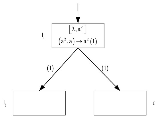
Figure 7. Deterministic ADD module, simulating ${\mathrm{l}}_{\mathrm{i}}:(\mathrm{A}\mathrm{D}\mathrm{D}(\mathrm{r}),{\mathrm{l}}_{\mathrm{j}})$.

Module FIN is omitted, but the instruction ${\mathrm{\sigma }}_{{\mathrm{l}}_{\mathrm{h}}}$ remains in system ${\mathrm{\Pi }}_2$. When neuron ${\mathrm{\sigma }}_{{\mathrm{l}}_{\mathrm{h}}}$ receives two spikes, it indicates that the halt instruction ${\mathrm{l}}_{\mathrm{h}}$ is reached, that is the register machine M halts.

Through the above description, we prove that system ${\mathrm{\Pi }}_2$ can correctly simulate the register machine M working in the accepting mode and can find that neurons of system ${\mathrm{\Pi }}_2$ contain at most two rules, Therefore, Theorem 2 holds.

4. DTNP-MCIR Systems as Function Computing Devices

In this part, we will discuss the ability of a small universal DTNP-MCIR system to calculate functions. A register machine $\mathrm{M}=\left(\mathrm{m},\mathrm{H},{\mathrm{l}}_0,{\mathrm{l}}_{\mathrm{h}},\mathrm{I}\right)$ is used to compute the function $\mathrm{f}:{\mathrm{N}}^{\mathrm{k}}\to \mathrm{N}$. Initially we assume that all registers are empty, k arguments are introduced into k registers. In general, only the first two registers are used. Then the register machine starts from the instruction ${\mathrm{l}}_0$ and continues to calculate until it reaches the halt instruction ${\mathrm{l}}_{\mathrm{h}}$. Finally, the function value is stored in a special register ${\mathrm{r}}_{\mathrm{t}}$. $\left({\mathsf{\phi }}_0,{\mathsf{\phi }}_1,\dots \right)$ is defined as a fixed admissible enumeration of the unary partial recursive functions. We think that a register machine is universal when there is a recursive function g that makes ${\mathsf{\phi }}_{\mathrm{X}}\left(\mathrm{y}\right)={\mathrm{M}}_{\mathrm{u}}\left(\mathrm{g}\left(\mathrm{x}\right),\mathrm{y}\right)$ for all natural numbers x, y.

Korec [31] proposed a small universal register machines ${\mathrm{M}}_{\mathrm{u}}=\left(8,\mathrm{H},{\mathrm{l}}_0,{\mathrm{l}}_{\mathrm{h}},\mathrm{I}\right)$. ${\mathrm{M}}_{\mathrm{u}}$ contains 8 registers (labeled from 0 to 8) and 23 instructions. By introducing two numbers g(x) and y into registers 1 and 2, respectively, ${\mathsf{\phi }}_{\mathrm{x}}(\mathrm{y})$ can be computed by ${\mathrm{M}}_{\mathrm{u}}$. When ${\mathrm{M}}_{\mathrm{u}}$ stops, the function value is stored in register 0. In order to simplify the register machine ${\mathrm{M}}_{\mathrm{u}}$, we introduce a new register 8 and replace the halt instruction with three new instructions: ${\mathrm{l}}_{22}:\left(\mathrm{S}\mathrm{U}\mathrm{B}(0),{\mathrm{l}}_{23},{\mathrm{l}}_{\mathrm{h}}\right)$; ${\mathrm{l}}_{23}:\left(\mathrm{A}\mathrm{D}\mathrm{D}(8),{\mathrm{l}}_{22}\right)$; ${\mathrm{l}}_{\mathrm{h}}:\mathrm{H}\mathrm{A}\mathrm{L}\mathrm{T}$. We define the modified register machine as ${\mathrm{M}}_{\mathrm{u}}{}^{\prime }$, as shown in Table 1. We will design a small universal DTNP-MCIR system to simulate the register machine ${\mathrm{M}}_{\mathrm{u}}{}^{\prime }$.

Table 1. Universal register machines ${\mathrm{M}}_{\mathrm{u}}{}^{\prime }$.

$\begin{array}{l}{\mathrm{l}}_0:\left(\mathrm{S}\mathrm{U}\mathrm{B}(1),{\mathrm{l}}_1,{\mathrm{l}}_2\right)\\ {\mathrm{l}}_2:\left(\mathrm{A}\mathrm{D}\mathrm{D}(6),{\mathrm{l}}_3\right)\\ {\mathrm{l}}_4:\left(\mathrm{S}\mathrm{U}\mathrm{B}(6),{\mathrm{l}}_5,{\mathrm{l}}_3\right)\\ {\mathrm{l}}_6:\left(\mathrm{S}\mathrm{U}\mathrm{B}(7),{\mathrm{l}}_7,{\mathrm{l}}_8\right)\\ {\mathrm{l}}_8:\left(\mathrm{S}\mathrm{U}\mathrm{B}(6),{\mathrm{l}}_9,{\mathrm{l}}_0\right)\\ {\mathrm{l}}_{10}:\left(\mathrm{S}\mathrm{U}\mathrm{B}(4),{\mathrm{l}}_0,{\mathrm{l}}_{11}\right)\\ {\mathrm{l}}_{12}:\left(\mathrm{S}\mathrm{U}\mathrm{B}(5),{\mathrm{l}}_{14},{\mathrm{l}}_{15}\right)\\ {\mathrm{l}}_{14}:\left(\mathrm{S}\mathrm{U}\mathrm{B}(5),{\mathrm{l}}_{16},{\mathrm{l}}_{17}\right)\\ {\mathrm{l}}_{16}:\left(\mathrm{A}\mathrm{D}\mathrm{D}(4),{\mathrm{l}}_{11}\right)\\ {\mathrm{l}}_{18}:\left(\mathrm{S}\mathrm{U}\mathrm{B}(4),{\mathrm{l}}_0,{\mathrm{l}}_{22}\right)\\ {\mathrm{l}}_{20}:\left(\mathrm{A}\mathrm{D}\mathrm{D}(0),{\mathrm{l}}_0\right)\\ {\mathrm{l}}_{22}:\left(\mathrm{S}\mathrm{U}\mathrm{B}(0),{\mathrm{l}}_{23},{\mathrm{l}}_{\mathrm{h}}\right)\\ {\mathrm{l}}_{\mathrm{h}}:\mathrm{H}\mathrm{A}\mathrm{L}\mathrm{T}\end{array}$

$\begin{array}{l}{\mathrm{l}}_1:\left(\mathrm{A}\mathrm{D}\mathrm{D}(7),{\mathrm{l}}_0\right)\\ {\mathrm{l}}_3:\left(\mathrm{S}\mathrm{U}\mathrm{B}(5),{\mathrm{l}}_2,{\mathrm{l}}_4\right)\\ {\mathrm{l}}_5:\left(\mathrm{A}\mathrm{D}\mathrm{D}(5),{\mathrm{l}}_6\right)\\ {\mathrm{l}}_7:\left(\mathrm{A}\mathrm{D}\mathrm{D}(1),{\mathrm{l}}_4\right)\\ {\mathrm{l}}_9:\left(\mathrm{A}\mathrm{D}\mathrm{D}(6),{\mathrm{l}}_{10}\right)\\ {\mathrm{l}}_{11}:\left(\mathrm{S}\mathrm{U}\mathrm{B}(5),{\mathrm{l}}_{12},{\mathrm{l}}_{13}\right)\\ {\mathrm{l}}_{13}:\left(\mathrm{S}\mathrm{U}\mathrm{B}(2),{\mathrm{l}}_{18},{\mathrm{l}}_{19}\right)\\ {\mathrm{l}}_{15}:\left(\mathrm{S}\mathrm{U}\mathrm{B}(3),{\mathrm{l}}_{18},{\mathrm{l}}_{20}\right)\\ {\mathrm{l}}_{17}:\left(\mathrm{A}\mathrm{D}\mathrm{D}(2),{\mathrm{l}}_{21}\right)\\ {\mathrm{l}}_{19}:\left(\mathrm{S}\mathrm{U}\mathrm{B}(0),{\mathrm{l}}_0,{\mathrm{l}}_{18}\right)\\ {\mathrm{l}}_{21}:\left(\mathrm{A}\mathrm{D}\mathrm{D}(3),{\mathrm{l}}_{18}\right)\\ {\mathrm{l}}_{23}:\left(\mathrm{A}\mathrm{D}\mathrm{D}(8),{\mathrm{l}}_{22}\right)\end{array}$

Theorem 3.

There is a small universal DTNP-MCIR system having 73 neurons for computing functions.

Proof. 

We design a DTNP-MCIR system ${\mathrm{\Pi }}_3$ to simulate the register machine ${\mathrm{M}}_{\mathrm{u}}{}^{\text{'}}$. System ${\mathrm{\Pi }}_3$ contains an INPUT module, an OUTPUT module, and some ADD and SUB modules to simulate the ADD and SUB instructions of ${\mathrm{M}}_{\mathrm{u}}{}^{\text{'}}$, respectively. The INPUT module is used to read the spike train from the environment, and the OUTPUT module deal with calculation result which is placed in register 8. Each register r and each instruction ${\mathrm{l}}_{\mathrm{i}}$ of ${\mathrm{M}}_{\mathrm{u}}{}^{\text{'}}$ corresponds to a neuron ${\mathrm{\sigma }}_{\mathrm{r}}$ and ${\mathrm{\sigma }}_{{\mathrm{l}}_{\mathrm{i}}}$ respectively. If the feeding input unit of neuron ${\mathrm{\sigma }}_{\mathrm{r}}$ contains 2n spikes, it means that the register r contains the number n. When neuron ${\mathrm{\sigma }}_{{\mathrm{l}}_{\mathrm{i}}}$ receives two spikes, the simulation of instruction ${\mathrm{l}}_{\mathrm{i}}$ is started. Initially, all neurons in system ${\mathrm{\Pi }}_3$ are assumed to be empty. □

The INPUT module is shown in Figure 8. The spike train ${10}^{\mathrm{g}\left(\mathrm{x}\right)}{10}^{\mathrm{y}}1$ is read from the environment by it, and 2g(x) spikes and 2y spikes will be stored in neurons ${\mathrm{\sigma }}_1$ and ${\mathrm{\sigma }}_2$ respectively. We do not use inhibitory rules in this module, but make full use of the function of multiple channels. Multiple channels have played a major role in saving neurons and improving system operation efficiency.

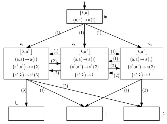
Figure 8. Module INPUT.

Suppose that neuron ${\mathrm{\sigma }}_{\mathrm{in}}$ receives the first spike form the environment at time ${\mathrm{t}}_1$.At time ${\mathrm{t}}_1+1$, rule $\left(\mathrm{a},\mathrm{a}\right)\to \mathrm{a}(1)$ is applied, and neuron ${\mathrm{\sigma }}_{\mathrm{in}}$ sends a spike to neurons ${\mathrm{\sigma }}_{{\mathrm{c}}_1}$,${\mathrm{\sigma }}_{{\mathrm{c}}_2}$ and ${\mathrm{\sigma }}_{{\mathrm{c}}_3}$. Since neurons ${\mathrm{\sigma }}_{{\mathrm{c}}_1}$, ${\mathrm{\sigma }}_{{\mathrm{c}}_2}$ and ${\mathrm{\sigma }}_{{\mathrm{c}}_3}$ all contain a spike, the rule $\left(\mathrm{a},\mathrm{a}\right)\to \mathrm{a}(1)$ in three neurons is enabled at time ${\mathrm{t}}_1+2$. That is, neuron ${\mathrm{\sigma }}_{{\mathrm{c}}_2}$ sends a spike to neuron ${\mathrm{\sigma }}_{{\mathrm{c}}_1}$, neuron ${\mathrm{\sigma }}_{{\mathrm{c}}_2}$ and neuron ${\mathrm{\sigma }}_{{\mathrm{c}}_3}$ exchange a spike with each other, as well as neuron ${\mathrm{\sigma }}_{{\mathrm{c}}_1}$ and neuron ${\mathrm{\sigma }}_{{\mathrm{c}}_2}$ each send a spike to neuron ${\mathrm{\sigma }}_1$ via channel (1). This process will repeat until the second spike reaches neuron ${\mathrm{\sigma }}_{\mathrm{in}}$. Therefore, neuron ${\mathrm{\sigma }}_1$ receives two spikes in each moment from time ${\mathrm{t}}_1+2$ to time $\mathrm{t}{}_1+\mathrm{g}\left(\mathrm{x}\right)+1$ and imports a total of $2\mathrm{g}\left(\mathrm{x}\right)$ spikes. (That is, the number stored in neuron ${\mathrm{\sigma }}_1$ is $\mathrm{g}\left(\mathrm{x}\right)$).

Assuming that the time for the second spike to reach neuron ${\mathrm{\sigma }}_{\mathrm{in}}$ is ${\mathrm{t}}_2$, in fact ${\mathrm{t}}_2=\mathrm{t}{}_1+\mathrm{g}\left(\mathrm{x}\right)+1$. Similarly, rule $\left(\mathrm{a},\mathrm{a}\right)\to \mathrm{a}(1)$ in neuron ${\mathrm{\sigma }}_{\mathrm{in}}$ is applied to send a spike to neurons ${\mathrm{\sigma }}_{{\mathrm{c}}_1}$, ${\mathrm{\sigma }}_{{\mathrm{c}}_2}$ and ${\mathrm{\sigma }}_{{\mathrm{c}}_3}$ at time ${\mathrm{t}}_2+1$. Then neurons ${\mathrm{\sigma }}_{{\mathrm{c}}_1}$, ${\mathrm{\sigma }}_{{\mathrm{c}}_2}$ and ${\mathrm{\sigma }}_{{\mathrm{c}}_3}$ each contain two spikes, so rule $\left({\mathrm{a}}^2,{\mathrm{a}}^2\right)\to \mathrm{a}(1)$ in neurons ${\mathrm{\sigma }}_{{\mathrm{c}}_1}$ and ${\mathrm{\sigma }}_{{\mathrm{c}}_3}$ is enabled and rule $\left({\mathrm{a}}^2,{\mathrm{a}}^2\right)\to {\mathrm{a}}^2(1)$ is applied in neurons ${\mathrm{\sigma }}_{{\mathrm{c}}_2}$ at time ${\mathrm{t}}_2+2$. Then neurons ${\mathrm{\sigma }}_{{\mathrm{c}}_1}$ and ${\mathrm{\sigma }}_{{\mathrm{c}}_3}$ respectively send a spike to neuron ${\mathrm{\sigma }}_2$ via channel(2) and exchange spikes with neuron ${\mathrm{\sigma }}_{{\mathrm{c}}_2}$ each step from this moment.

Neuron ${\mathrm{\sigma }}_2$ receives a total of 2y spikes from time ${\mathrm{t}}_2+2$ to time $\mathrm{t}{}_2+\mathrm{y}+1$ (That is, the number stored in neuron ${\mathrm{\sigma }}_2$ is y). When the third spike is imported by neuron ${\mathrm{\sigma }}_{\mathrm{in}}$, the next moment neurons ${\mathrm{\sigma }}_{{\mathrm{c}}_1}$,${\mathrm{\sigma }}_{{\mathrm{c}}_2}$, and ${\mathrm{\sigma }}_{{\mathrm{c}}_3}$ will each contain three spikes. Three spikes are consumed by forgetting rule $\left({\mathrm{a}}^3,\mathrm{\lambda }\right)\to \mathrm{\lambda }$ in neuron ${\mathrm{\sigma }}_{{\mathrm{c}}_2}$ and ${\mathrm{\sigma }}_{{\mathrm{c}}_3}$. Rule $\left({\mathrm{a}}^3,\mathrm{\lambda }\right)\to {\mathrm{a}}^2\left(3\right)$ in neuron ${\mathrm{\sigma }}_{{\mathrm{c}}_1}$ is applied to transmit two spikes to neuron ${\mathrm{\sigma }}_{{\mathrm{l}}_0}$ via channel (3), this indicates that the system ${\mathrm{\Pi }}_3$ starts to simulate the initial instruction ${\mathrm{l}}_0$.

By observing Table 1, we can find that all ADD instructions have the form ${\mathrm{l}}_{\mathrm{i}}:(\mathrm{A}\mathrm{D}\mathrm{D}(\mathrm{r}),{\mathrm{l}}_{\mathrm{j}})$, therefore, we use the deterministic ADD module shown in Figure 7 to simulate the ADD instructions. Its working mechanism has been clarified in the proof of Theorem 2.

In addition, the SUB instruction ${\mathrm{l}}_{\mathrm{j}}:(\mathrm{S}\mathrm{U}\mathrm{B}(\mathrm{r}),{\mathrm{l}}_{\mathrm{j}},{\mathrm{l}}_{\mathrm{k}})$ can be simulated by the SUB module in Figure 4. The working mechanism of the SUB module has been discussed during the proof of Theorem 1.

When neuron ${\mathrm{\sigma }}_{{\mathrm{l}}_{\mathrm{h}}}$ receives two spikes at time t, the calculation of the system ${\mathrm{\Pi }}_3$ halts. The OUTPUT module shown in Figure 9 is used to deal with the calculation results. We assume that neuron ${\mathrm{\sigma }}_8$ contains 2n spikes. The configuration of OUTPUT module at time t is ${{\mathrm{C}}_{\mathrm{t}}}^{‴}=\left(\left[{\mathrm{u}}_1,{\mathrm{\tau }}_1\right],\left[{\mathrm{u}}_2,{\mathrm{\tau }}_2\right],\dots ,\left[{\mathrm{u}}_5,{\mathrm{\tau }}_5\right],\right)$, which involves fives neurons ${\mathrm{\sigma }}_{{\mathrm{l}}_{\mathrm{h}}},{\mathrm{\sigma }}_{{\mathrm{c}}_1},{\mathrm{\sigma }}_{{\mathrm{c}}_2},{\mathrm{\sigma }}_8,{\mathrm{\sigma }}_{\mathrm{o}\mathrm{u}\mathrm{t}}$ respectively. Thus, ${{\mathrm{C}}_{\mathrm{t}}}^{‴}=\left(\left[2,2\right],\left[0,1\right],\left[0,1\right],\left[2\mathrm{n},1\right],\left[0,1\right]\right)$. Rule $\left({\mathrm{a}}^2,\mathrm{a}\right)\to \mathrm{a}(1)$ is enabled, and neuron ${\mathrm{\sigma }}_{{\mathrm{l}}_{\mathrm{h}}}$ sends one spike to neurons ${\mathrm{\sigma }}_{{\mathrm{c}}_1},{\mathrm{\sigma }}_{{\mathrm{c}}_2}$ and ${\mathrm{\sigma }}_8$ via channel (1) at time t. Therefore, ${\mathrm{C}}_{\mathrm{t}+1}^{‴}=\left(\left[0,2\right],\left[1,1\right],\left[1,1\right],\left[2\mathrm{n}+1,1\right],\left[0,1\right]\right)$. Since neuron ${\mathrm{\sigma }}_{{\mathrm{c}}_2}$ is the inhibitory neuron of neuron ${\mathrm{\sigma }}_{{\mathrm{c}}_1}$ and ${\mathrm{u}}_{{\mathrm{c}}_2}\left(\mathrm{t}+1\right)={\mathrm{\tau }}_{{\mathrm{c}}_1}\left(\mathrm{t}+1\right)$, rule $\left(\mathrm{a},\overline{\mathrm{a}}\right)\to \mathrm{a}(1)$ is applied, neuron ${\mathrm{\sigma }}_{{\mathrm{c}}_1}$ sends a spike to neuron ${\mathrm{\sigma }}_{\mathrm{o}\mathrm{u}\mathrm{t}}$. Rule $\left(\mathrm{a},\mathrm{a}\right)\to \mathrm{a}(1)$ in neuron ${\mathrm{\sigma }}_{{\mathrm{c}}_2}$ and rule ${\mathrm{a}}^{2\mathrm{b}+1}/\left({\mathrm{a}}^3,\mathrm{a}\right)\to \mathrm{a}(1)$ in neuron ${\mathrm{\sigma }}_8$ are also enabled. Although the rule ${\mathrm{a}}^{2\mathrm{b}+1}/\left({\mathrm{a}}^3,\mathrm{a}\right)\to \mathrm{a}(1)$ consumes three spikes of neuron ${\mathrm{\sigma }}_8$, because neuron ${\mathrm{\sigma }}_8$ and neuron ${\mathrm{\sigma }}_{{\mathrm{c}}_2}$ exchange one spike with each other via channel (1), neuron ${\mathrm{\sigma }}_8$ only consumes two spikes each moment. Thus, ${\mathrm{C}}_{\mathrm{t}+2}^{‴}=\left(\left[0,2\right],\left[0,1\right],\left[1,1\right],\left[2\mathrm{n}-1,1\right],\left[1,1\right]\right)$. Rule $\left(\mathrm{a},\mathrm{a}\right)\to \mathrm{a}(1)$ is applied in neuron ${\mathrm{\sigma }}_{\mathrm{o}\mathrm{u}\mathrm{t}}$, then the first spike is sent to the environment at time t + 2. Rule ${\mathrm{a}}^{2\mathrm{b}+1}/\left({\mathrm{a}}^3,\mathrm{a}\right)\to \mathrm{a}(1)$ will be executed continuously until neuron ${\mathrm{\sigma }}_8$ contains only one spikes. At time t + n + 1, neuron ${\mathrm{\sigma }}_8$ contains only a spike, rule ${\mathrm{a}}^{2\mathrm{b}+1}/\left(\mathrm{a},\mathrm{a}\right)\to \mathrm{a}(2)$ is applied and neuron ${\mathrm{\sigma }}_8$ transmits a spike to neuron ${\mathrm{\sigma }}_{\mathrm{o}\mathrm{u}\mathrm{t}}$ via channel (2). At time t + n + 2, rule $\left(\mathrm{a},\mathrm{a}\right)\to \mathrm{a}(1)$ is applied, neuron ${\mathrm{\sigma }}_{\mathrm{o}\mathrm{u}\mathrm{t}}$ sends the second spike to the environment. According to the definition in Section 2, the result of the system ${\mathrm{\Pi }}_3$ is $\mathrm{n}=\left(\mathrm{t}+\mathrm{n}+2\right)-\left(\mathrm{t}+2\right)$, which is also the number contained in register 8.

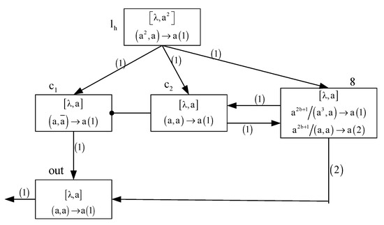
Figure 9. OUTPUT module.

From the above description, it can be seen that the system ${\mathrm{\Pi }}_3$ can correctly simulate the register machine ${\mathrm{M}}_{\mathrm{u}}{}^{\text{'}}$ calculation function. System ${\mathrm{\Pi }}_3$ contains a total of 81 neurons: (1) the INPUT module has 3 auxiliary neurons; (2) the OUTPUT module has 2 auxiliary neurons; (3) each SUB module has 3 auxiliary neurons, for a total of 42 neurons; (4) 9 neurons correspond to 9 registers; (5) 25 neurons correspond to 25 instructions.

We can further reduce the number of neurons in system ${\mathrm{\Pi }}_3$ by combining instructions. Here are three cases:

Case 1. For the sequence of two consecutive ADD instructions ${\mathrm{l}}_{17}:\left(\mathrm{A}\mathrm{D}\mathrm{D}(2),{\mathrm{l}}_{21}\right)$ and ${\mathrm{l}}_{21}:\left(\mathrm{A}\mathrm{D}\mathrm{D}(3),{\mathrm{l}}_{18}\right)$, we can use the model ADD-ADD in Figure 10 to simulate so that neuron ${\mathrm{\sigma }}_{{\mathrm{l}}_{21}}$ corresponding to instruction ${\mathrm{l}}_{21}$ can be saved.

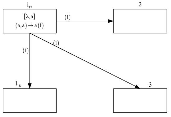
Figure 10. The model simulating consecutive ADD-ADD instructions ${\mathrm{l}}_{17}:\left(\mathrm{A}\mathrm{D}\mathrm{D}(2),{\mathrm{l}}_{21}\right)$ and ${\mathrm{l}}_{21}:\left(\mathrm{A}\mathrm{D}\mathrm{D}(3),{\mathrm{l}}_{18}\right)$.

Case 2. We can also combine instructions ${\mathrm{l}}_{15}:\left(\mathrm{S}\mathrm{U}\mathrm{B}(3),{\mathrm{l}}_{18},{\mathrm{l}}_{20}\right)$ and ${\mathrm{l}}_{20}:\left(\mathrm{A}\mathrm{D}\mathrm{D}(0),{\mathrm{l}}_0\right)$ to form one instruction ${\mathrm{l}}_{15}:\left(\mathrm{S}\mathrm{U}\mathrm{B}(3),{\mathrm{l}}_{18},\left(\mathrm{A}\mathrm{D}\mathrm{D}\left(0\right),{\mathrm{l}}_0\right)\right)$ so that ${\mathrm{\sigma }}_{{\mathrm{l}}_{20}}$ will be saved. The SUB-ADD-1 model shown in Figure 11 can be used to simulate newly formed instructions.

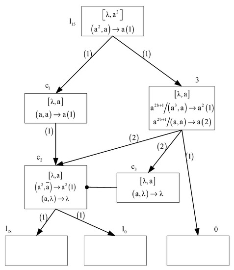
Figure 11. The model simulating consecutive SUB-ADD-1 instructions ${\mathrm{l}}_{15}:\left(\mathrm{S}\mathrm{U}\mathrm{B}(3),{\mathrm{l}}_{18},{\mathrm{l}}_{20}\right)$ and ${\mathrm{l}}_{20}:\left(\mathrm{A}\mathrm{D}\mathrm{D}(0),{\mathrm{l}}_0\right)$.

Case 3. The following six pairs of ADD and SUB instructions can be combined.

$$\begin{gathered} {\mathrm{l}}_0:\left(\mathrm{S}\mathrm{U}\mathrm{B}(1),{\mathrm{l}}_1,{\mathrm{l}}_2\right),{\mathrm{l}}_1:\left(\mathrm{A}\mathrm{D}\mathrm{D}(7),{\mathrm{l}}_0\right); \\ {\mathrm{l}}_4:\left(\mathrm{S}\mathrm{U}\mathrm{B}(6),{\mathrm{l}}_5,{\mathrm{l}}_3\right),{\mathrm{l}}_5:\left(\mathrm{A}\mathrm{D}\mathrm{D}(5),{\mathrm{l}}_6\right); \\ {\mathrm{l}}_6:\left(\mathrm{S}\mathrm{U}\mathrm{B}(7),{\mathrm{l}}_7,{\mathrm{l}}_8\right),{\mathrm{l}}_7:\left(\mathrm{A}\mathrm{D}\mathrm{D}(1),{\mathrm{l}}_4\right); \\ {\mathrm{l}}_8:\left(\mathrm{S}\mathrm{U}\mathrm{B}(6),{\mathrm{l}}_9,{\mathrm{l}}_0\right),{\mathrm{l}}_9:\left(\mathrm{A}\mathrm{D}\mathrm{D}(6),{\mathrm{l}}_{10}\right); \\ {\mathrm{l}}_{14}:\left(\mathrm{S}\mathrm{U}\mathrm{B}(5),{\mathrm{l}}_{16},{\mathrm{l}}_{17}\right),{\mathrm{l}}_{16}:\left(\mathrm{A}\mathrm{D}\mathrm{D}(4),{\mathrm{l}}_{11}\right); \\ {\mathrm{l}}_{22}:\left(\mathrm{S}\mathrm{U}\mathrm{B}(0),{\mathrm{l}}_{23},{\mathrm{l}}_{\mathrm{h}}\right),{\mathrm{l}}_{23}:\left(\mathrm{A}\mathrm{D}\mathrm{D}(8),{\mathrm{l}}_{22}\right); \end{gathered}$$

By observing the above six pairs of instructions, it can be seen that the latter ADD instruction is at the position of the first exit of the previous SUB instruction. Therefore, the combination instructions can be expressed as ${\mathrm{l}}_{\mathrm{i}}:\left(\mathrm{S}\mathrm{U}\mathrm{B}\left({\mathrm{r}}_1\right),{\mathrm{l}}_{\mathrm{j}},{\mathrm{l}}_{\mathrm{k}}\right),{\mathrm{l}}_{\mathrm{j}}:\left(\mathrm{A}\mathrm{D}\mathrm{D}\left({\mathrm{r}}_2\right),{\mathrm{l}}_{\mathrm{g}}\right)$. In this way, we can save six neurons. The recombined SUB and ADD instructions can be simulated by the SUB-ADD-2module in Figure 12.

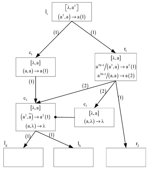
Figure 12. The model simulating consecutive SUB-ADD-2 instructions ${\mathrm{l}}_{\mathrm{i}}:\left(\mathrm{S}\mathrm{U}\mathrm{B}\left({\mathrm{r}}_1\right),{\mathrm{l}}_{\mathrm{j}},{\mathrm{l}}_{\mathrm{k}}\right),{\mathrm{l}}_{\mathrm{j}}:\left(\mathrm{A}\mathrm{D}\mathrm{D}\left({\mathrm{r}}_2\right),{\mathrm{l}}_{\mathrm{g}}\right)$.

In summary, we can save eight neurons in total by combining some ADD/SUB instructions. The recombined instructions can be simulated with ADD-ADD, SUB-ADD-1and SUB-ADD-2modules respectively. Therefore, the number of neurons in system ${\mathrm{\Pi }}_3$ dropped from 81 to 73. So far, we have completed the proof of Theorem 3.

In order to further illustrate the computing power of DTNP-MCIR systems, we compared it with some computing models in term of small number of computing units. From Table 2, we can see that DTNP systems, SNP systems, SNP-IR systems and recurrent neural networks need 109,67,100 and 886 neurons respectively to achieve Turing universality for computing function. However, DTNP-MCIR systems need fewer neurons than them. Although SNP-MC systems require only 38 neurons to compute function, which is much less than the computing unit required by DTNP-MCIR systems, they have different working modes. SNP-MC systems work in asynchronous mode but DTNP-MCIR systems work in synchronous mode. Therefore, the comparison indicates that DTNP-MCIR systems need fewer neurons than most of modes. In addition, Table 3 gives the full name of the comparative model abbreviation.

Table 2. The comparison of different computing models in the term of small number of computing units.

Computing Models	Computing Functions
DTNP-MCIR systems	73
DTNP systems [29]	109
SNP systems [32]	67
SNP-IR systems [28]	100
Recurrent neural networks [33]	886
SNP-MC systems [34]	38

Table 3. Abbreviations and corresponding full names of some systems cited in the paper.

DTNP systems [29]	Dynamic threshold neural P systems
SNP-IR systems [28]	Spiking neural P systems with inhibitory rules
SNP-MC systems [27]	Spiking neural P systems with multiple channels
SNP systems [32]	Smaller universal spiking neural P systems
SNP-MC systems [34]	Small universal asynchronous spiking neural P systems with multiple channels.

5. Conclusions and Further Work

Inspired by SNP systems with inhibitory rules (SNP-IR systems) and the learning of SNP systems with multiple channels (SNP-MC systems), this paper proposes a dynamic threshold neural P system with inhibitory rules and multiple channels (DTNP-MCIR systems). In fact, dynamic threshold neural P systems (DTNP systems) had been researched and proved to be Turing universal number generating/accepting device. Our original intention to construct DTNP-MCIR systems is to more fully simulate the actual situation of neurons communicating through synapses, and also to show the use of inhibitory rules and multiple channels in DTNP systems. In addition, we have optimized DTNP systems. The form of firing rules is ${\mathrm{E}}_{\mathrm{i}}/\left({\mathrm{a}}^{\mathrm{u}},{\mathrm{a}}^{\mathrm{\tau }}\right)\to {\mathrm{a}}^{\mathrm{p}}$, where $\mathrm{u}\ge 1,\mathrm{\tau }\ge 0,\mathrm{p}\ge 0$, and $\mathrm{p}\le \mathrm{u}$. However, $\mathrm{\tau }$ and $\mathrm{p}$ are always equal in the DTNP system, we think it lacks generality and improve it; For the rule $\left({\mathrm{a}}^{\mathrm{u}},{\mathrm{a}}^{\mathrm{\tau }}\right)\to {\mathrm{a}}^{\mathrm{p}}$ of neuron ${\mathrm{\sigma }}_{\mathrm{r}}$ in the SUB module, If neuron ${\mathrm{\sigma }}_{\mathrm{r}}$ contains 2n spikes at time t and $2\mathrm{n}\ge \mathrm{u}$, then neuron ${\mathrm{\sigma }}_{\mathrm{r}}$ can be fired at time t, which is unreasonable for the entire system. Therefore, we improve the form of firing rules as ${\mathrm{a}}^{2\mathrm{b}+1}/\left({\mathrm{a}}^{\mathrm{u}},{\mathrm{a}}^{\mathrm{\tau }}\right)\to {\mathrm{a}}^{\mathrm{p}}(1)$, where ${\mathrm{a}}^{2\mathrm{b}+1}$ is a regular expression we introduced, which means that neuron ${\mathrm{\sigma }}_{\mathrm{r}}$ can be fired only when the number of spikes is an odd number.

In the future, we want to research whether DTNP-MCIR systems can be combined with certain algorithms, we think that the two data units of DTNP-MCIR systems can be used as two parameter inputs, the use of inhibitory rules and multiple channels make them have stronger control capabilities. Moreover, because DTNP-MCIR systems are a distributed parallel computing model, they can greatly improve the computational efficiency of algorithms. Future work will focus on using DTNP-MCIR systems to solve real-world problems, such as image processing and data clustering

References

- Păun, G. Computing with membranes. J. Comput. Syst. Sci. 2000, 61, 108–143. [Google Scholar] [CrossRef]
- Song, T.; Gong, F.; Liu, X. Spiking neural P systems with white hole neurons. IEEE Trans. NanoBiosci. 2016, 15, 666–673. [Google Scholar] [CrossRef]
- Freund, R.; Păun, G.; Pérez-Jiménez, M.J. Tissue-like P systems with channel-states. Theor. Comput. Sci. 2005, 330, 101–116. [Google Scholar] [CrossRef]
- Song, T.; Pan, L.; Wu, T. Spiking neural P Systems with leaning functions. IEEE Trans. NanoBiosci. 2019, 18, 176–190. [Google Scholar] [CrossRef] [PubMed]
- Cabarle, F.G.C.; Adorna, H.N.; Jiang, M.; Zeng, X. Spiking neural P systems with scheduled synapses. IEEE Trans. NanoBiosci. 2017, 16, 792–801. [Google Scholar] [CrossRef] [PubMed]
- Song, T.; Pan, L. Spiking neural P systems with rules on synapses working in maximum spiking strategy. IEEE Trans. NanoBiosci. 2015, 14, 465–477. [Google Scholar] [CrossRef]
- Ionescu, M.; Păun, G.; Yokomori, T. Spiking neural P systems. Fund. Inform. 2006, 71, 279–308. [Google Scholar]
- Song, T.; Pan, L. Spiking neural P systems with request rules. Neurocomputing 2016, 193, 193–200. [Google Scholar] [CrossRef]
- Zeng, X.; Zhang, X. Spiking Neural P Systems with Thresholds. Neural Comput. 2014, 26, 1340–1361. [Google Scholar] [CrossRef]
- Zhao, Y.; Liu, X. Spiking Neural P Systems with Neuron Division and Dissolution. PLoS ONE 2016, 11, e0162882. [Google Scholar] [CrossRef]
- Wang, J.; Shi, P.; Peng, H.; Perez-Jimenez, M.J.; Wang, T. Weighted Fuzzy Spiking Neural P Systems. IEEE Trans. Fuzzy Syst. 2012, 21, 209–220. [Google Scholar] [CrossRef]
- Jiang, K.; Song, T.; Pan, L. Universality of sequential spiking neural P systems based on minimum spike number. Theor. Comput. Sci. 2013, 499, 88–97. [Google Scholar] [CrossRef]
- Zhang, X.; Luo, B. Sequential spiking neural P systems with exhaustive use of rules. Biosystems 2012, 108, 52–62. [Google Scholar] [CrossRef] [PubMed]
- Cavaliere, M.; Ibarra, O.H.; Păun, G.; Egecioglu, O.; Ionescu, M.; Woodworth, S. Asynchronous spiking neural P systems. Theor. Comput. Sci. 2009, 410, 2352–2364. [Google Scholar] [CrossRef]
- Song, T.; Pan, L.; Păun, G. Asynchronous spiking neural P systems with local synchronization. Inf. Sci. 2013, 219, 197–207. [Google Scholar] [CrossRef]
- Song, T.; Zou, Q.; Liu, X.; Zeng, X. Asynchronous spiking neural P systems with rules on synapses. Neurocomputing 2015, 151, 1439–1445. [Google Scholar] [CrossRef]
- Păun, G. Spiking neural P systems with astrocyte-like control. J. Univers. Comput. Sci. 2007, 13, 1707–1721. [Google Scholar]
- Wu, T.; Păun, A.; Zhang, Z.; Pan, L. Spiking Neural P Systems with Polarizations. IEEE Trans. Neural Netw. Learn. Syst. 2017, 29, 3349–3360. [Google Scholar]
- Păun, A.; Păun, G. Small universal spiking neural P systems. BioSystems 2007, 90, 48–60. [Google Scholar] [CrossRef]
- Cabarle, F.; Adorna, H.; Perez-Jimenez, M.; Song, T. Spiking neuron P systems with structural plasticity. Neural Comput. Appl. 2015, 26, 1905–1917. [Google Scholar] [CrossRef]
- Peng, H.; Chen, R.; Wang, J.; Song, X.; Wang, T.; Yang, F.; Sun, Z. Competitive spiking neural P systems with rules on synapses. IEEE Trans. NanoBiosci. 2017, 16, 888–895. [Google Scholar] [CrossRef] [PubMed]
- Xiong, G.; Shi, D.; Zhu, L.; Duan, X. A new approach to fault diagnosis of power systems using fuzzy reasoning spiking neural P systems. Math. Probl. Eng. 2013, 2013, 1–13. [Google Scholar] [CrossRef]
- Wang, T.; Zhang, G.X.; Zhao, J.B.; He, Z.Y.; Wang, J.; Pérez-Jiménez, M.J. Fault diagnosis of electric power systems based on fuzzy reasoning spiking neural P systems. IEEE Trans. Power Syst. 2015, 30, 1182–1194. [Google Scholar] [CrossRef]
- Peng, H.; Wang, J.; Ming, J.; Shi, P.; Pérez-Jiménez, M.J.; Yu, W.; Tao, C. Fault diagnosis of power systems using intuitionistic fuzzy spiking neural P systems. IEEE Trans. Smart Grid. 2018, 9, 4777–4784. [Google Scholar] [CrossRef]
- Peng, H.; Wang, J.; Shi, P.; Pérez-Jiménez, M.J.; Riscos-Núñez, A. An extended membrane system with active membrane to solve automatic fuzzy clustering problems. Int. J. Neural Syst. 2016, 26, 1–17. [Google Scholar] [CrossRef] [PubMed]
- Zhang, G.; Rong, H.; Neri, F.; Pérez-Jiménez, M. An optimization spiking neural P system for approximately solving combinatorial optimization problems. Int. J. Neural Syst. 2014, 24, 1440006. [Google Scholar] [CrossRef] [PubMed]
- Peng, H.; Yang, J.; Wang, J.; Wang, T.; Sun, Z.; Song, X.; Lou, X.; Huang, X. Spiking neural P systems with multiple channels. Neural Netw. 2017, 95, 66–71. [Google Scholar] [CrossRef] [PubMed]
- Peng, H.; Li, B.; Wang, J. Spiking neural P systems with inhibitory rules. Knowl.-Based Syst. 2020, 188, 105064. [Google Scholar] [CrossRef]
- Peng, H.; Wang, J. Dynamic threshold neural P systems. Knowl.-Based Syst. 2019, 163, 875–884. [Google Scholar] [CrossRef]
- Peng, H.; Wang, J. Coupled Neural P Systems. IEEE Trans. Neural Netw. Learn. Syst. 2019, 30, 1672–1682. [Google Scholar] [CrossRef]
- Korec, I. Small universal register machines. Theor. Comput. Sci. 1996, 168, 267–301. [Google Scholar] [CrossRef]
- Zhang, X.; Zeng, X.; Pan, L. Smaller universal spiking neural P systems. Fundam. Inf. 2007, 87, 117–136. [Google Scholar]
- Siegelmann, H.T.; Sontag, E.D. On the computational power of neural nets. J. Comput. Syst. 1995, 50, 132–150. [Google Scholar] [CrossRef]
- Song, X.; Peng, H. Small universal asynchronous spiking neural P systems with multiple channels. Neurocomputing 2020, 378, 1–8. [Google Scholar] [CrossRef]
© 2020 by the authors. Licensee MDPI, Basel, Switzerland. This article is an open access article distributed under the terms and conditions of the Creative Commons Attribution (CC BY) license (http://creativecommons.org/licenses/by/4.0/).