Abstract
The turbulence intensity (TI) is defined as the ratio of fluctuation from the standard deviation of wind velocity to the mean value. Many studies have been performedon TI for flow dynamics and adapted various field such as aerodynamics, jets, wind turbines, wind tunnel apparatuses, heat transfer, safety estimation of construction, etc.The TI represents an important parameter for determining the intensity of velocity variation and flow quality in industrial fluid mechanics. In this paper, computational fluid dynamic (CFD) simulation of TI alteration with increasing temperature has been performed using the finite volume method. A high-temperature—maximum 300 degrees Celsius (°C)—wind tunnel test rig has been used as theapparatus, and velocity was measured by an I-type hot-wire anemometer. The velocity and TI of the core test section were operated at several degrees of inlet temperatures at anair velocity of 20 m/s. The magnitude of TI has a relationship with boundary layer development. The TI increased as temperature increased due to turbulence created by the non-uniformities.
1. Introduction
The turbulence intensity (TI) representsa primary parameter for determining the intensity of wind velocity variation according to the ratio of fluctuation from the standard deviation of wind velocity to the mean value. The ratio reflects the importance of the element for wind-related phenomena such as buffeting, vortex-induced vibration, flutter, and galloping [1]. Many studies have been performedon TI for various fields in industrial fluid mechanics. Cook (2013) derived TI at varying altitudes for aircraft flight stability in a non-steady atmosphere for aerodynamics [2]. The longitudinal TI applied in jetswas studied and the mean-flow and turbulence properties simulated by Dejoan et al. [3]. Barthelmie et al. researched detailed wind resources including TI for wind turbines and overviewed the state of the art in wind resource assessment with modeling and measurement techniques [4]. Moreover, TI has been the principal data in the production of electricity from wind energy [5]. The heat and mass transfer across the membrane considering TI was researched by Zhang [6], and Ahn et al. investigated the intrinsically unsteady heat transfer on the surface of a cylinder in crossflowin detail by numerical simulation as a function of the freestream TI [7].
In 2014, Silva et al. reviewed different TI interfacial layers, including the flow variable as velocity, and researched the flow dynamics which determine the growth, spreading, mixing, and reaction rates in many flows of engineering and natural interest [8]. Nishi et al. studied the environmental and boundary layer of a wind tunnel to control turbulence characteristics [9]. Kelberlau et al.estimated the TI with a continuous wave wind lidar [10], and Yang et al. studied the aerodynamic characteristics of a gurney flap in turbulence level (TI of 0.2%, 10.5%, and 19.0%) [11].
Basse studied TI with the friction factor from pipe flow measurements made in the Princeton Superpipe [12,13]. Wind tunnels are experimental devices to simulate certain flow conditions and to study the flow over objects of interest. The TI is one of the important parameters to estimate the flow quality inside the wind tunnel [14]. While setting boundary conditions for turbulence computational fluid dynamic (CFD) simulation, it is required to estimate the TI on the inlets [15]. L. Pareschi and M. Zanella proposed a novel numerical approach for computational fluid dynamics for aspace-homogeneous case, as temperature variation is taken into account and treated as an uncertain quantity [16].
Moreover, TI could be one of the most significant indicators indetermining the completeness of wind tunnel design and production.Despite this, few studieshave been reported for the measurement of TI, considering the temperature increases. In this research, computational fluid dynamic (CFD) simulation of TI alteration with increasing temperature is used with the finite element method and experimental research under a certain freestream velocity. A high-temperature—up to 200 degreesCelsius (°C)—wind tunnel test rig has beendesigned as the apparatus, and velocity was measured by I-type hot-wire anemometer. The velocity and TI of the core test section were operated at several degrees of inlet temperatures at an air velocity of 20 m/s.
2. Computational Fluid Dynamics
In order to guarantee a reliable mode of estimation for TI in the wind tunnel, numerical simulations have to be investigated quantitatively. The analysis of velocity profiles according to temperature increases was carried out using the finite volume method using ANSYS Fluent [17].
The governing equations of computational fluid dynamics are continuity, momentum and energy conservation, as in Equations (1)–(3), respectively
Where ( = 1,2,3) is the tensor notation of subscripts and , and is the velocity vector, is the pressure and is the temperature, respectively. , and are the density, specific heat at constant pressure and coefficient of thermal conductivity. Moreover, Reynolds-averagedNavier–Stokes equationsare used and is shown is Equation (4)
The standard k- model wasapplied for fully developed flow simulation with a two-dimensional (2D) steady state, considering the appropriate calculation. The transport equation for the standard k- model which was applied in numerical analysis is shown in Equation (5)
where, represents the generation of turbulence kinetic energy due to the mean velocitygradients, calculated as described in modeling turbulent production in the k- models. isthe generation of turbulence kinetic energy due to buoyancy, calculated as described in the effects ofbuoyancy on turbulence in the k- models. represents the contribution of the fluctuatingdilatation in compressible turbulence to the overall dissipation rate, calculated as described in the effectsof compressibility on turbulence models. , , and are constants and , are the turbulent Prandtl numbers for and , respectively. and are user-defined source terms and the turbulent viscosity, , is calculated by and , as in Equation (6)
is constant, and the model constant value = 1.44, = 1.92, = 0.09, = 1.0, = 1.3 was accepted in this numerical simulation [18]. The boundary condition configured as the experimental condition with an inlet velocity of 20 m/s and an interior hot film probe region was applied. Figure 1 shows the modeling and number of 51,200 grids for computational simulation, and the boundary conditions and model parametersare listed in Table 1.
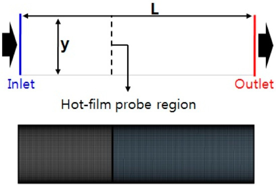
Figure 1.
Schematic diagram of modeling and grid for simulation.

Table 1.
The boundary conditions and model parameters.
Nevertheless, as the TI increases, the change in velocity distribution on the wall surface becomes noticeable and it is considered that the effect of TI is greater than the inlet temperature. For efficient calculation, numerical simulation was conducted to check whether the 2D and 3D result values were consistent, and the results are shown in Figure 2.
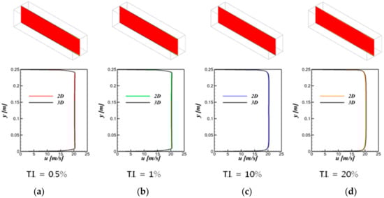
Figure 2.
The comparison of 2D and 3D result for various turbulence intensities(TI); (a) 0.5%, (b) 1%, (c) 10%, (d) 20%.
Moreover, compared to TI, the velocity boundary layer is not affected by the inlet temperature change. Figure 3 shows the velocity profile of various TIswhen increasing the temperature. The velocity gradient slightly decreases as the inlet temperature increases due to the Reynolds number decreasing according to the viscosity, which increaseswith temperature. The comparison result of the velocity profile for temperature increases in certain TIs is shown in Figure 4, and the velocity distribution near the boundary layer is relatively significant.
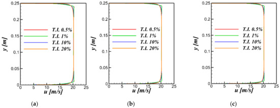
Figure 3.
Velocity profile of various TI for the temperature; (a) 25, (b) 100, (c) 200 °C.
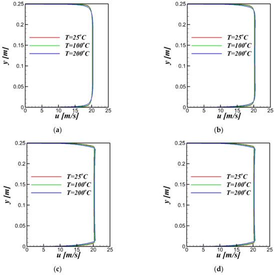
Figure 4.
Velocity profile of temperature increases for the TI; (a) 0.5%, (b) 1%, (c) 10%, (d) 20%.
3. Experiments
Wind tunnels which can be regarded as applicable under high temperature have a maximum temperate of 300 °C, whereas nominal wind tunnels are used under normal ambient temperature. Figure 5 shows the schematic diagram of the comprehensive test equipment for a high-temperature wind tunnel including the test section where the TI is measured in certain conditions. The experiments provide a uniform free stream wind velocity of 20 m/s from a blower with a generation capacity of to the test section, passing 300 kW power consumption, with an electric heater through an inlet diffuser, with a honeycomb structure.
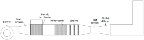
Figure 5.
Schematic diagram of comprehensive test system of TI.
Figure 6 shows a schematic diagram of the test section with a square cross-sectional area of 250 × 250 mm beneath the hot-wire probe. The 2D traverse device has been attached for measuring the velocity in the vertical(y) and horizontal (L) direction. The hot-wire measurement system consists of a sensor, a small electrically heated wire exposed to the fluid flow, and electronic equipment which performs the transformation of the sensor output into a useful electrical signal. The I-type hot-wire probe’s (Model 1220 High Temperature Straight Probe, TSI) specifications are shown in Figure 7, which measured the velocity and TI for a maximum temperature of 300 °C.
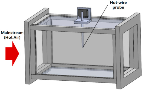
Figure 6.
Schematic diagram of test section and hot wire probe.
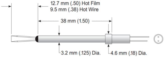
Figure 7.
Specification of I-type hot wire probe.
4. Result and Discussion
In order to examine the variation of TI according to the inlet flow temperature, the test was conducted by changing the inlet air flow temperature from atmospheric temperature to 200 °C. Figure 8 shows the result of the TI distribution in the longitudinal and horizontal direction. The temperature of inlet flow was 25 °C, and the velocity of the core of the main flow was 20 m/s. In location at the middle of the wind tunnel, at which y = 125 mm, the TI was 0.36% and increased near the wall, as shown in CFD. In addition, the magnitude of TI has a relationship with boundary layer development. At x/L = 0.6, where boundary layer is developing, the TI was 1.75% at y = 5mm. At x/L = 1, where the boundary layer is fully developed, it was 3.5% at the same altitude. The TI at the inlets for internal flows is generally dependent on the upstream history of the flow. Figure 9 shows the experiment results of the TI value according to the temperature increasing at the core of the wind tunnel test section at the free stream velocity of 20 m/s. As temperature increased, the TI increased slightly. The measured average TI values are 0.36%, 0.6%, and 0.98% at the temperature of 25, 100, 200 °C, respectively. Note that the experiment’s TI values were very low for a lab-scale wind tunnel.
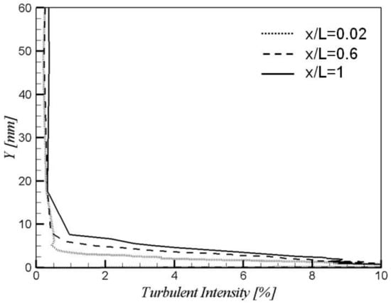
Figure 8.
TI distribution of near the wall for wind velocity of 20 m/s.
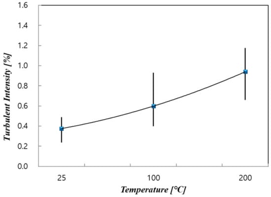
Figure 9.
TI measurement increasing the temperature; 25 to 200 °C.
5. Conclusions
This study addresses the numerical simulation and experimental measurement of TI under an approaching free stream velocity with a high temperature gradient using a hot-wire anemometer. The influence of temperature is reflected in the TI values induced by the shear and its diffusion due to the turbulence generated. The stronger the shear becomes, the higher the level of turbulence with TI. The effect of free stream TI is more apparent on temperature change. The TI is slightly increased as temperature increases, and the magnitude of TI is related to boundary layer development due to the turbulence created by the non-uniformities.
Author Contributions
J.L. built up the research project, designed the experiments and performed investigation; J.-H.L. contributed to the search process, formal analysis and wrote the paper. All authors have read and agreed to the published version of the manuscript.
Funding
This work was supported by National Research Foundation of Korea (NRF) grant funded by the Korea government (MSIP; Ministry of Science, ICT & Future Planning) (No. 2017R1C1B5076422).
Conflicts of Interest
The authors declare no conflict of interest.
References
- Kimura, K. Innovative Bridge Design Handbook; Elsevier: Amsterdam, The Netherlands, 2016; pp. 37–48. [Google Scholar]
- Cook, M.V. Flight Dynamics Principles: A Linear Systems Approach to Aircraft Stability And Control; Elsevier: Amsterdam, The Netherlands, 2013; pp. 4–444. [Google Scholar]
- Dejoan, A.; Leschziner, M.A. Large eddy simulation of a plane turbulent wall jet. Phys. Fluids 2005, 17, 025102. [Google Scholar] [CrossRef]
- Barthelmie, R.J.; Pryor, S.C. Meteorology and wind resource assessment for wind farm development. Wind Energy Syst. 2011, e28, 3–27. [Google Scholar]
- Sørensen, J.D.; Sørensen, J.N. Wind Energy Systems. Woodhead Publ. Ser. Energy 2011, 1, 46–111. [Google Scholar]
- Silva, C.; Hunt, J.; Eames, I.; Westerweel, J. Interfacial Layers Between Regions of Different Turbulence Intensity. Ann. Rev. Fluid Mech. 2014, 46, 567–590. [Google Scholar] [CrossRef]
- Zhang, L.Z. Conjugate Heat and Mass Transfer in Heat Mass Exchanger Ducts; Academic Press: Cambridge, MA, USA, 2013; pp. 181–232. [Google Scholar]
- Ahn, J.; Sparrow, E.M.; Gorman, J.M. Turbulence intensity effects on heat transfer and fluid-flow for a circular cylinder in crossflow. Int. J. Heat Mass Transf. 2017, 113, 613–621. [Google Scholar] [CrossRef]
- Nishih, A.; Miyagi, H.; Higuchi, K. A Computer-Controlled Wind Tunnel. In Proceedings of the 1st International Symposium on Computational Wind Engineering (CWE 92), Tokyo, Japan, 21–23 August 1993; pp. 837–846. [Google Scholar]
- Kelberlau, F.; Neshaug, V.; Lønseth, L.; Bracchi, T.; Mann, J. Taking the Motion out of Floating Lidar: Turbulence Intensity Estimates with a Continuous-Wave Wind Lidar. Remote Sens. 2020, 12, 898. [Google Scholar] [CrossRef]
- Yang, J.; Yang, H.; Zhu, W.; Li, N.; Yuan, Y. Experimental Study on Aerodynamic Characteristics of a Gurney Flap on a Wind Turbine Airfoil under High Turbulent Flow Condition. Appl. Sci. 2020, 10, 7258. [Google Scholar] [CrossRef]
- Basse, N.T. Turbulence intensity and the friction factor for smooth- and rough-wall pipe flow. Fluids 2017, 2, 30. [Google Scholar] [CrossRef]
- Basse, N.T. Turbulence Intensity Scaling: A Fugue. Fluids 2019, 4, 180. [Google Scholar] [CrossRef]
- Mahta, R.D.; Bradshaw, P. Design rules for small low speed wind tunnels. Aeronaut. J. 1979, 83, 442–449. [Google Scholar]
- Cattafesta, L.; Bahr, C.; Mathew, J. Fundamentals of Wind-Tunnel Design. Exp. Tech. Fluid Dyn. Ther. Sci. 2010, 1–10. [Google Scholar] [CrossRef]
- Pareschi, L.; Zanella, M. Monte Carlo stochastic Galerk in methods for the Boltzmann equation with uncertainties: space-homogeneous case. J. Comput. Phys. 2020, 423, 109822. [Google Scholar] [CrossRef]
- Lee, J.S.; Seo, Y.M.; Jeong, C.H.; Kim, M.S.; Park, Y.G.; Ha, M.Y. Numerical analysis and design optimization of engine room to improve cooling performance for a mid-class excavator. J. Mech. Sci. Technol. 2019, 33, 3265–3275. [Google Scholar] [CrossRef]
- ANSYS. Fluent Theory Guide Release 15.0; ANSYS, Inc.: Canonsburg, PA, USA, 2013; pp. 47–48. [Google Scholar]


Publisher’s Note: MDPI stays neutral with regard to jurisdictional claims in published maps and institutional affiliations. |
© 2020 by the authors. Licensee MDPI, Basel, Switzerland. This article is an open access article distributed under the terms and conditions of the Creative Commons Attribution (CC BY) license (http://creativecommons.org/licenses/by/4.0/).