Review

Challenges and Opportunities on Nonlinear State Estimation of Chemical and Biochemical Processes

1
Department of Chemical and Biomedical Engineering, West Virginia University, Morgantown, WV 26506, USA
2
Department of Engineering, Federal University of Lavras, Lavras, MG 37200-900, Brazil
*
Author to whom correspondence should be addressed.
Processes 2020, 8(11), 1462; https://doi.org/10.3390/pr8111462
Submission received: 17 October 2020 / Revised: 9 November 2020 / Accepted: 11 November 2020 / Published: 15 November 2020
(This article belongs to the Special Issue Feature Review Papers)

Abstract

:
This paper provides an overview of nonlinear state estimation techniques along with a discussion on the challenges and opportunities for future work in the field. Emphasis is given on Bayesian methods such as moving horizon estimation (MHE) and extended Kalman filter (EKF). A discussion on Bayesian, deterministic, and hybrid methods is provided and examples of each of these methods are listed. An approach for nonlinear state estimation design is included to guide the selection of the nonlinear estimator by the user/practitioner. Some of the current challenges in the field are discussed involving covariance estimation, uncertainty quantification, time-scale multiplicity, bioprocess monitoring, and online implementation. A case study in which MHE and EKF are applied to a batch reactor system is addressed to highlight the challenges of these technologies in terms of performance and computational time. This case study is followed by some possible opportunities for state estimation in the future including the incorporation of more efficient optimization techniques and development of heuristics to streamline the further adoption of MHE.

1. Introduction

Modern chemical and biochemical plants must satisfy technical, economic, and environmental requirements that have become increasingly challenging. Stronger economic competition and sustainable development goals have imposed stringent environmental and safety regulations, as well as the need for more profitable plant operation and tighter product quality specifications. In this scenario, process monitoring, estimation, and control have gained increased attention, driving the development of new technologies to operate modern plants safely and profitably.
Process monitoring plays a key role among the technologies related to process control. Measuring instruments and mathematical tools are generally employed to monitor process variables, providing online state/output information for feedback control systems and for detecting abnormal process operations. When online measurements of state variables are noisy or not available in practice, mathematical tools known as state estimators can be used to reconcile noisy data and estimate missing variables [1,2].
A considerable amount of literature has been published on the development and application of state estimators to improve monitoring of chemical [3,4,5,6,7,8,9,10] and biochemical [11,12,13,14] processes. Previous research and review articles have also covered state estimation aspects in terms of classification [1,15,16], design, and applications [1,17,18], as well as challenges and trends on nonlinear state estimation [1,16,19,20].
This paper aims to present a current overview of the main nonlinear state estimators used to monitor chemical and biochemical processes. A systematic approach is proposed to design nonlinear state estimators in general, from the problem definition to the system analysis and performance evaluation, with a focus on Bayesian estimators. Such an approach provides guidelines to practitioners when designing or improving control and monitoring systems. Challenges and opportunities are also discussed on covariance estimation, uncertainty quantification, time-scale multiplicity, bioprocess monitoring, online implementation, and the incorporation of computationally efficient optimization solvers associated with nonlinear state estimators.
The rest of the paper is structured as follows. First, a brief historical perspective on the main contributions to the estimation theory is presented, as well as a general and practical approach to design and test state estimators. Then, some important challenges on nonlinear state estimation are discussed. This discussion is followed by a section containing a nonlinear batch reactor case study for illustrating extended Kalman filter (EKF) and moving horizon estimation (MHE) implementations. Based upon the authors’ perspective, opportunities and trends in the development of nonlinear state estimation are finally outlined, followed by the conclusions.

2. Nonlinear State Estimation Background and Design

2.1. State of the Art

State estimation refers to a set of mathematical techniques designed to reconstruct the state information of a system. In particular, unmeasured state variables are estimated based on available model output predictions and noisy measurements. The main challenge in the state estimation task is to provide reliable online estimation under process and measurement uncertainties while being computationally tractable. Process uncertainties usually come from plant-model mismatch and disturbances, whereas measurement noises are mainly related to the instrument’s precision. Figure 1 presents a schematic diagram of state estimation that consists of two main stages: model prediction (i.e., a priori state estimate) and measurement update (i.e., a posteriori estimate, based on current and past measured variables). Past estimates may also be used in recursive estimation algorithms.
Historically, Thomas Bayes was the first main contributor to the state estimation field by proposing the Bayesian rule in the eighteenth century, which is the basis for statistical inference methods [21]. Some decades later, Carl Friedrich Gauss developed the technique of least-squares estimation applied to the inference of parameters related to the orbit of planets [22]. Another significant contribution to the estimation theory occurred in 1912, when Fisher introduced the maximum likelihood estimation approach [23]. Three decades later, Kolmogorov and Wiener independently proposed the linear minimum mean-square error estimator, which formed the basis for the forthcoming recursive estimation theory [24,25]. Then, in 1960, Rudolf Kalman conceived an optimal recursive filter based on the state-space domain, known as the Kalman filter (KF) [26], whose estimates are obtained considering linear dynamic models and online measurements. For the implementation of the KF formulation on nonlinear systems, extensions such as extended Kalman filter (EKF) [9] and unscented Kalman filter (UKF) [27] were later developed based on model linearizations at different time steps and nonlinear transformations, respectively. In addition to nonlinearity, many chemical and biochemical systems may also be subject to hard constraints (e.g., nonnegative level, pressure, and concentration) and present non-Gaussian noise distributions (e.g., asymmetric or multi-modal probability densities), for which standard Kalman filtering may no longer be applicable. As the original EKF and UKF formulations are unable to directly handle constraints, modifications have been proposed to these algorithms [28,29,30]. Constraints may also be addressed using state estimation methods developed more recently, such as moving horizon estimation (MHE) [31] and particle filtering (PF) [32].
MHE is an optimization-based technique that minimizes the sum of squared errors between past measurements and state/output predictions over a N -length sliding window, weighted by the covariance matrices associated with the state and measurement uncertainties [31]. The finite sliding-estimation window in MHE is a way to overcome the computational burden associated with solving the full information problem (that considers the entire trajectory of states) online, where the information prior to the sliding window is represented by the arrival cost term [17]. As an optimization-based method, MHE is able to deal explicitly with system constraints, providing improved robustness for several process applications [3,5,6,11,13]. However, computational cost in the MHE implementation for large-scale industrial processes is still a challenge today, due to the requirement of solving nonlinear optimization problems online at every time step.
PF, in turn, is an example of a recursive method that handles nonlinear dynamic systems with non-normally distributed state and measurement noises [32]. Due to these features, PF has gained increasing attention for nonlinear state estimation of a number of chemical process applications [16,33,34,35]. In this method, the state a posteriori probability density is represented by a set of random samples (or particles), which are able to capture the time-varying nature of non-Gaussian distributions recursively without the need of approximating the process model [32]. However, PFs may be sensitive to poor initial guesses and display robustness issues due to plant-model mismatch [17]. Even though increasing the number of samples might improve PF estimates, this strategy may become intractable in practice, even for systems with reasonably small state dimensions [9]. Thus, the combination of PF with MHE has been explored as a hybrid approach that provides the advantages of the former (fast estimation) and the latter (robustness to poor initial guesses and unmodeled disturbances) [9,17,36].
In general, the main state estimators applied to nonlinear chemical and biochemical systems can be divided into three groups: Bayesian, deterministic, and hybrid methods. Figure 2 provides a schematic diagram with the general classification of these nonlinear estimation methods, further described in the paragraphs below.
Bayesian methods assume that the process states and measurements are subject to random disturbances. This is the most popular class of state estimators used for chemical processes. The estimation procedure is essentially based on finding the conditional probability distribution of the state and output variables, described mathematically by Bayes’ rule and characterized by parameters such as mean and covariance [17]. The Bayesian approach may be divided into two subgroups: recursive and optimization-based methods. Recursive methods consist of single-step estimators that are typically unconstrained and fast. However, they may not be robust to the presence of data outliers, unmodeled disturbances, and model errors. Extended Kalman filter (EKF), unscented Kalman filter (UKF), and particle filter (PF) are some of the most popular recursive estimation algorithms [3,27,32,37,38,39,40]. Optimization-based approaches may use a sliding window of measurements that provides improved robustness. These estimators can also incorporate hard state constraints, such as nonnegative concentrations and pressures, into the problem formulation. Moving horizon estimator (MHE) is the main representative of the optimization-based methods. This category of estimation techniques will produce the same results as the recursive methods when considering an unconstrained, linear, infinite horizon length optimization problem, as the least-squares optimization problem solution is identical to the solution from maximizing the conditional density function for Gaussian noises [3,9,31,41,42].
Deterministic methods, by contrast, are based on the assumption that both measurement and state variables are deterministic, i.e., system outputs can be considered to be fully determined by the operating conditions (initial conditions and inputs) and the parameter values in the process models. The deterministic approaches can be further divided into two subgroups: first-order systems (FOS)-based and artificial intelligence (AI)-based methods. FOS-based estimators are designed for systems whose dynamics are represented by linearized differential equations of first-order nature. Extended Luenberger and asymptotic observers are the main state estimators under this subgroup. The extended Luenberger observer (ELO) is characterized by the addition of a correction term, that is proportional to the error between the measured and the estimated states, to the differential equation model. The proportional gain is chosen in such a way that the error dynamics is stable at the zero-observation error case [43]. This estimator has been successfully used for systems described by accurate process models (i.e., considering perfect knowledge of the system parameters) [1,3,44,45]. The asymptotic observer (AO), in turn, takes advantage of the dynamic model structure to rewrite the differential equation system, for example independently of the process kinetics [44]. Thus, this estimator is indicated for specific cases in which the process kinetics (e.g., reaction and heat transfer rates) are unknown [46,47,48]. However, the asymptotic observer is stable and convergent only for fed-batch and continuous operating systems (i.e., for non-zero dilution rates) [43]. AI-based estimators are an alternative to tackle complex and ill-defined problems using algorithms based on artificial intelligence, such as artificial neural networks (ANN) and fuzzy logic. These techniques, once trained with real data, are able to provide fast estimates based on information of the process inputs and measurements. These estimators have been increasingly employed for biochemical processes applications [49,50,51,52]. However, AI-based methods may demand additional time and efforts for formulation and fail when subjected to unmodeled conditions.
Hybrid methods combine two or more estimation technologies, either as part of an integrated framework or to perform different tasks in the estimation procedure. Examples of the latter are the use of AI-based methods to describe the process dynamics (modeling task), combined with Bayesian algorithms to carry out the estimation task, taking into account the stochastic nature of the system [14,53,54,55]. On the other hand, integrated frameworks considering, for instance, EKF/PF-MHE may use time-efficient technologies, such as EKF and PF, to obtain fast state estimates between MHE optimizations, which are robust to bad priors and unmodeled disturbances [13,17,36]. Therefore, the hybrid approach combines the best features of the estimation technologies and potentially overcomes the limitations of a single-based estimator design. Since the year 2000, hybrid state estimators have been increasingly developed for chemical and biochemical processes, which suggests the future trend towards the design of hybrid state estimators for nonlinear systems [1].

2.2. Approach for Nonlinear State Estimation Design

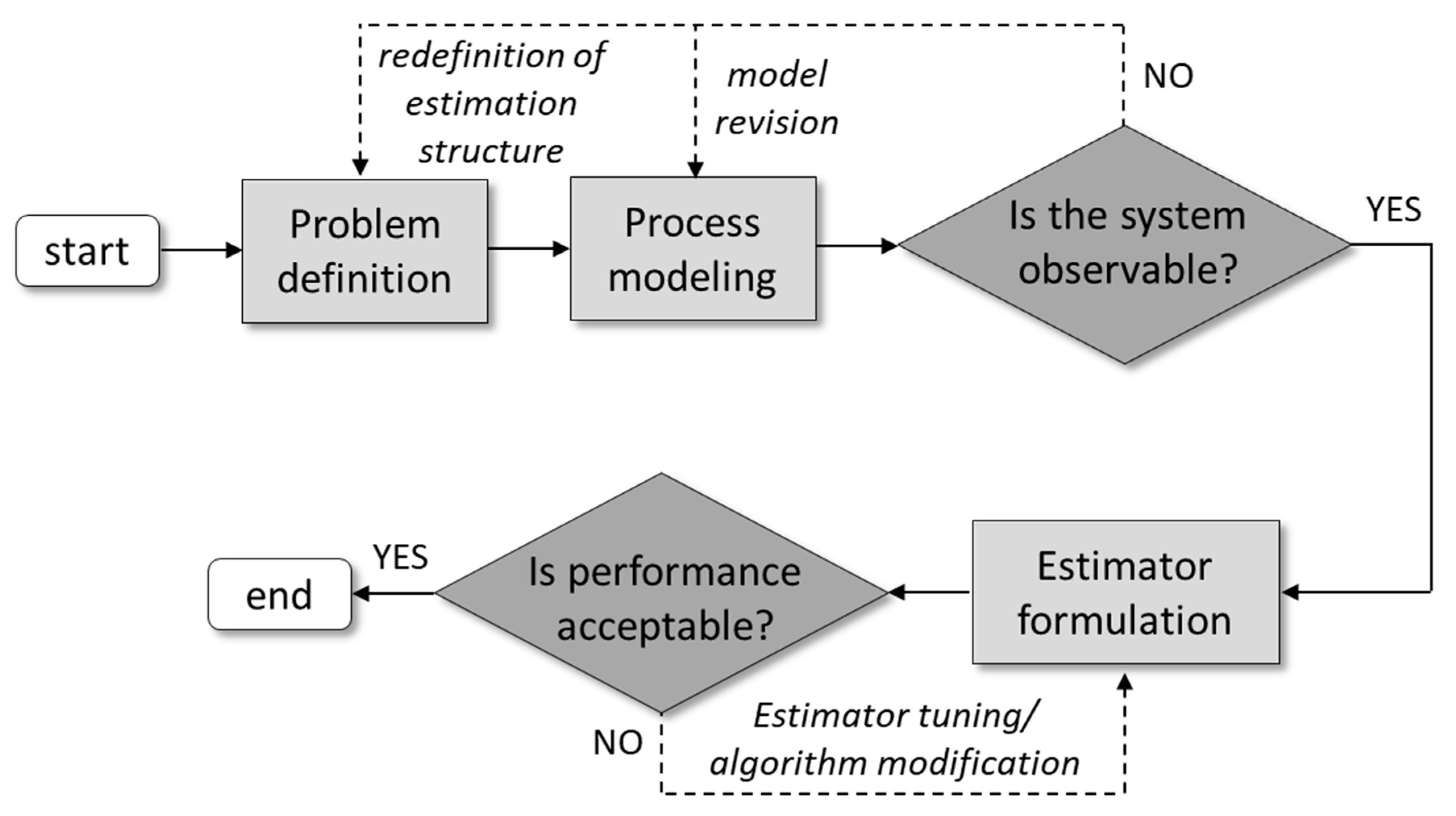
When designing a state estimator for a given nonlinear system, a list of tasks must be carried out. These tasks can be gathered in five major steps: (i) problem definition, (ii) process modeling, (iii) observability assessment, (iv) estimator formulation, and (v) performance evaluation. The proposed approach outlined in Figure 3 is suggested as a general guideline to assist researchers and practitioners in the design of nonlinear state estimators.
As the first step, the estimation problem must be defined. In particular, given a system, one should identify the relevant process inputs and outputs. In addition, it is recommended to separate the measurable states from those whose online measurements are not available or reliable in practice. Based on this step, the process states intended to be estimated are selected. It is worth mentioning that model parameters, as well as process inputs, may also be estimated online by properly adapting the state estimators [56,57]. However, this article is focused on the estimation of process states.
The next step concerns the development of the process model, i.e., the derivation of equations that describe the system dynamics (dynamic model), or simply its static behavior according to the operating conditions (steady-state model). Process modeling is based on the definition of the model structure (e.g., dynamic, static, order, etc.), followed by model fitting (e.g., parameter identification from experimental data) and validation (model checking based on training and new fresh data sets) [58]. In essence, process models may be fully derived from first principles (e.g., energy and mass balances), defined as white box models, purely data-driven (black box models), or a combination of both (gray box models) [50]. For Bayesian estimators, the main focus in this article, the nonlinear model should be discrete and stochastic, in which the states x k can be represented by the deterministic model, F, integrated over a sampling time t = t k + 1 t k , with added process noises, w k , to cope with potential plant-model mismatches as shown in Equation (1) [15]. The measured outputs, y k , can be represented as a function of the states, h, with added measurement noises, υ k , as in Equation (2). Process and measurement noises are generally assumed to be Gaussian with mean zero and covariance Q and R , respectively [15]. The developed models should relate the measured outputs to the unmeasured/estimated states, as a necessary (but not sufficient) condition for the system observability, which is assessed in the following step.
x k + 1 = F ( x k , u k ) + G k w k
y k = h ( x k ) + υ k
in which x R n , y R p , and u R m are the process states, measured outputs, and input variables, respectively. G k = G ( x k ) is the disturbance model that maps the process noises to state variables [5].
The third stage consists of checking the system observability. A system is observable if every state x ( t 0 ) can be determined from the information of the inputs u ( t ) and measurements y ( t ) over a finite time interval t [ t 0 , t ] [59]. While the mathematical formulation of nonlinear observability is well defined in the literature [9], a full analysis in this case is often intractable. For practical applications, local observability may be adopted, and a necessary condition for local observability of a discrete-time nonlinear system at time t k is that the n p × n observability matrix O in Equation (3) is of rank n [60]. As the observability of the dynamic system is dependent on its structure, a directed graph can be constructed to represent the dynamic system, and the structural observability of the system can be checked based on the association between the measured system outputs and the state variables using graph theory [61]. For a large-scale system, when the observability matrix suffers from ill-conditioning, structural observability can be evaluated using a bond-graph approach, in which the linearized system is transformed into a structurally equivalent system with Boolean coefficients [62]. The sensitivity matrices A k , B k , and C k are derived from the linearization of the process and measurement models at the corresponding time t k , according to Equations (4)–(6). If the necessary condition for local observability is not satisfied, the system is said to be unobservable and a revision of the process and/or measurement models as well as state estimation structure may be needed.
O = [ C k C k A k C k A k n 1 ] n p × n
x k + 1 = F ( x k , u k ) + G k w k A k x k + B k u k + G k w k
y k = h ( x k ) + υ k C k x k + υ k
A k = F x | x k , u k ;   B k = F u | x k , u k ;   C k = h x | x k
The fourth step aims at the state estimator formulation. The first task here is to select the estimation technology to be employed. A useful guideline is proposed in reference [1] to help designers in the selection of appropriate state estimators according to the knowledge on the system dynamics and parameters. Computational cost, stochastic nature of the system, and the quality of initial guesses for the states and covariances may also influence the choice of the estimation technology. After selecting the estimator, its implementation usually requires the adjustment of the tuning parameters, which impacts the estimation performance. For Bayesian estimators, the process and measurement noise covariance matrices ( Q and R , respectively) are the tuning parameters. These matrices can be adjusted manually or automatically by employing advanced algorithms, such as the autocovariance least-squares (ALS) technique [4,5,6,15].
In the final stage, the estimation performance can be evaluated through simulations followed by the online implementation [3,5,6]. For simulation testing, the process can be simulated using stochastic models, with the addition of process and measurement noises (as in Equations (1) and (2)) [15]. Scenarios of poor initial guesses, high measurement noise, plant-model mismatch, and unmeasured disturbances may be simulated [13]. The performance of the state estimators can be assessed and compared with respect to the estimation accuracy and computational cost, quantified by the mean squared error (MSE) in Equation (7) and the average computation time taken for each iteration (CPU-time), respectively [3,13,39,63]. In the case of unsatisfactory results, one can readjust the tuning parameters or try another estimation technology.
M S E = 1 N k = 1 N ( x k x ^ k ) T ( x k x ^ k )
in which x k and x ^ k denote the actual and estimated states, respectively, at time t k , with k = 1 , 2 , , N . In practice, the actual state values are often unknown and thus may be substituted in this formulation by the measured variables or the process model simulation states.

3. Challenges on Nonlinear State Estimation

3.1. Covariance Estimation

Many of the state estimation techniques used today are reliant on accurate estimates of both the process noise covariances and measurement noise covariances. As far back as the 1960s, years after the introduction of Kalman filtering, researchers emphasized that imperfect approximations can lead to significantly higher peak variances, slower convergence, and overall suboptimal estimation performance [64,65]. Despite these issues, it is commonplace in industrial applications to simply provide arbitrary covariance values, as it is often challenging to quantify model and measurement uncertainty in real processes [4].
Although there is no de facto way of deriving process noise and system noise covariances, there is an extensive amount of literature that attempts to address this challenge. Often, each of these methods requires different assumptions about the linearity (or lack thereof) of the plant model, the number of system noises, observability conditions, etc.
Modern covariance estimation techniques can be divided into four categories: correlation techniques, maximum likelihood methods, covariance matching methods, and Bayesian methods [66,67]. Of these four methods, both Bayesian and maximum likelihood methods have fallen out of favor for online use due to their large computational time [67].
The correlation-based methods include modern estimation techniques such as autocovariance least-squares (ALS). ALS has gone through several revisions and has been extended to nonlinear and time-varying models from its initial debut where only linear models were considered [15,67,68]. This flexibility has allowed ALS to be applied to both high dimensional nonlinear processes and batch processes with excellent successes, as demonstrated in the literature [4,5,6].
One of the more popular covariance matching methods used today for both linear time-invariant and linear time-variant systems is the noise covariance matrices estimation with gaussianity assessment (NEGA) method [66,69]. Based on the reported references, this method was used for linear systems and has the unique feature of performing a statistical test to examine the Gaussian property of the noises [66,69]. This is important as many estimation methods, such as the EKF and MHE, require Gaussian noise distributions.
A more in-depth analysis and overview of covariance estimation was published in 2017 [70]. That publication emphasized correlation-based methods but also introduced other techniques, and can serve as a basis of other survey papers that focus on those techniques. Overall, there are an extensive number of covariance estimation techniques that can be used to generate accurate and reliable measurement and system covariances for both linear and nonlinear processes with the main challenges related to the method selection and potential complexity for implementation.

3.2. Uncertainty Quantification

Uncertainty quantification remains an important challenge in nonlinear state estimation, as a parametrically distributed disturbance (such as a Gaussian noise) can result in a non-standard output measurement. Uncertainty quantification in state estimation can be categorized into two major types: forward uncertainty propagation and inverse uncertainty quantification. While these two classes of problems are correlated, the main objective of the first class is designing a model that accurately represents the real dynamic stochastic process, and the second class focuses on finding the state variables and the parameters of the system’s model from available measurements. Typically, the models are formulated in a form of a Hidden Markov Model (HMM) as a prerequisite of a recursive estimation algorithm. HMM assumes that the current uncertainty is only affected by the immediately previous time’s uncertainty, which allows a faster update of the current time distribution. HMM contains two stochastic processes, in which one cannot be measured directly (“hidden”) and the other is a conditional process of the first process’s realization. The hidden stochastic process represents the state evolution of a discrete-time first-principles model or black-box model and possesses the Markov property to ensure that the current uncertainty only propagates to the following time. The second stochastic process serves as the model of the measurement with probabilistic errors. Alternatively, the effects of unaccounted measurements in a distant past are accounted for with an arrival cost function, such as for the case of the MHE [31]. Additionally, the models can be designed to ensure the conjugacy to maintain the similarity between the prior and the posterior distribution, and the posterior distribution can be quickly updated online. The benefit of a conjugate model can be recognized in a linear time-invariant system with a Kalman filter, where the calculation of the estimated means of the estimated covariance matrix gives the full information on the probability density function of the state variables.
Mathematical models become more flexible when some parameters are considered to be time-variant. However, this approach introduces a new source of uncertainty called parameter uncertainty, which is distinct from process disturbances and measurement errors, and its effects need to be considered in the formulation of the nonlinear state estimation problem. Some approaches of simultaneously estimating the parameters along with the states are discussed in the literature, and a common approach corresponds to augmenting the parameters as pseudo-state variables [71], as already mentioned in Section 3.1. Different variations in Kalman filters can be applied to this augmented system, such as EKF [72,73], UKF [74], ensemble KF [75], and Kitanidis KF [76]. Additionally, optimization-based dual estimation approaches can be constructed similarly to the MHE [77] or with a moving window likelihood maximization [78].
Polynomial chaos was first introduced by Wiener as another method of propagating uncertainty without the need for sampling the prior [79], and the generalized polynomial chaos (gPC) was developed for various continuous and discrete distributions using orthogonal polynomials [80]. Even though the calculation of the coefficients of gPC, which often requires solving an online optimization problem, in parameter and state estimation frameworks typically takes more time than a sequence of important sampling methods, the overall online computational time of gPC approaches is shorter due to their fast prediction [81]. Additionally, the coefficients of gPC are sufficient to calculate the moments of the state variables [82], so they can be used to calculate the measurement update and the prediction step of the EKF [83] and ensemble KF [84].
In practice, the nonlinearity of the dynamic process often results in some non-Gaussian distributed outputs, which can be approximated by a finite convex sum of Gaussian distributions based on the Wiener approximation theorem [20]. This type of uncertainty modeling can be defined as a Gaussian Mixture (GM) model, and it is typically used for multimodal stochastic processes. When the system dynamics are linear or marginally nonlinear, only the GM’s weights of the initial states are updated when the measurement data arrive using a Bayesian recursion [85,86]. The new weights are calculated from the minimization of the integral square errors of the prediction and true probability density function [87] and using maximum a posteriori estimation [88]. For nonlinear continuous-time systems, the exact forecast of the state probability density function is given by the solution of the Fokker–Planck–Kolmogorov linear partial differential equation [89], and various numerically approximated solutions are available [87,90,91,92]. For practical applications, a more efficient solution of the Fokker–Planck–Kolmogorov equations for a multiple input and output system still remains challenging to obtain. Alternatively, a conjugate structure of the disturbance model for nonlinear systems needs further research to be able to quickly update the uncertainty’s probability density function calculation.

3.3. Time-Scale Multiplicity

Much of the literature published on estimation lacks emphasis on systems where the dynamics vary significantly between parts of the system. An example of this occurring is on highly integrated systems in which mass and energy balance dynamics may occur at vastly different rates. Traditionally, these systems are described using differential-algebraic equations (DAE). In such systems of equations, the differential equations characterize the slower dynamics, while the algebraic equations characterize the fast dynamics. The uniqueness of this type of system often requires the use of specialized estimation techniques.
To specifically address nonlinear DAE systems, a set of modifications to the original EKF were proposed by references [93,94]. The main limitation of this work was the inability to incorporate measurements of algebraic states into the recursive algorithm. This limitation was resolved in references [95,96], as both algebraic and differential states could be measured and used to update the state estimates. In this algorithm, once new estimates are obtained for both the algebraic and differential states, only the differential states are retained. The algebraic states are re-estimated by solving the algebraic equations using the original filter estimates.
Work has also been conducted to deal with DAEs by employing MHE-based approaches such as in reference [97], where the Tennessee Eastman process (a benchmark estimation problem) was solved online using a multiple shooting technique. In this direct multiple shooting method, the DAE is relaxed using a set of equality constraints embedded in the online MHE problem. The time-scale multiplicity is overcome by increasing the number of partitions of the time interval to have a more accurate representation of the process’s time integration. However, too many partition points may increase the complexity of the parameter estimation problem, thus challenging the method tractability for online implementation.
Additional MHE methods for addressing multi-rate systems have been published [8], in which the covariance matrix is updated using nonlinear programming sensitivity. An alternative approach published in reference [7] considers the decomposition of a two-time scale system into two separate reduced-order systems using a distributed moving horizon state estimation (DMHE) method. An interesting challenge that remains to be solved is on how to define when a system transitions into a time-scale multiplicity case. For example, how different do the system dynamics need to be before a system is classified as a DAE? Does a system become a DAE when the dynamics vary by at least three orders of magnitude, four orders of magnitude, etc.? Such a challenge provides opportunities for further research in state estimation under time-scale multiplicity.

3.4. Bioprocess Monitoring

Bioprocesses are usually subject to a highly nonlinear and time-varying influence of process variables, including temperature, pressure, pH level, and concentrations of substrate, product, inducers, and inhibitors. Minor adjustments to these variables often lead to abrupt changes to the dynamics of the cells’ growth and production rates, as well as the enzyme kinetics [98]. Thus, in order to ensure the high quality and reproducibility of bioprocesses, it is imperative to accurately monitor and control key process variables, as outlined by the Process Analytical Technology (PAT) initiative [99,100].
The design and implementation of reliable control systems is based on accurate, precise, and real-time measurements of selected variables. The real-time measuring of the variables such as pH level and the oxygen and carbon dioxide compositions in the bioreactor (gas and liquid phases) is well established and utilizes affordable sensors. However, the composition of further compounds may not be measured online due to the high price of the sensors (e.g., impedance, infrared, Raman, and mass spectrometers) or even the lack of suitable measurement devices. Even when these sensors are used, they are subject to significant noise, making it hard to directly infer the concentration of certain compounds. Examples of such variables are the concentrations of reactants and products of enzymatic reactions or entire metabolic pathways, as well as the physiological state of cells. As a consequence, those process variables are usually measured only a few times a day in industrial plants, or even in research laboratories, by manual sampling and time-consuming analysis (i.e., at-line and off-line measurements) [101,102]. In this context, the use of nonlinear state estimators in conjunction with direct state measurements can enable the reliable bioprocess monitoring and control [103,104].
The development of state estimators for bioprocesses is a challenging task owing to the increased complexity of such systems, mainly associated with their highly nonlinear and time-varying dynamics. Consequently, the adequate description of the dynamics of the enzyme kinetics, or the cells’ growth and production rates, usually involves nonlinear process models with a large number of parameters (that may be time-dependent or not) [105,106]. Moreover, single models are often valid only in a limited period of time or range of operating conditions [13,52,107,108]. A generic nonlinear and time-varying mathematical model to describe bioprocesses dynamics is illustrated in Equation (8).
d x d t = f ( x , u , t ) = { f 1 ( x , u , θ 1 ( t ) ) ;   i f   [ x X 1 ,   u U 1 ,   t T 1 ] f 2 ( x , u , θ 2 ( t ) ) ;   i f   [ x X 2 ,   u U 2 ,   t T 2 ] f j ( x , u , θ j ( t ) ) ;   i f   [ x X j ,   u U j ,   t T j ]
in which θ j ( t ) R q are time-varying parameters. X j , U j , and T j are specific ranges of process states, input variables, and process time, respectively.
Over the past few decades, several studies have proposed promising techniques to overcome the challenges related to the state estimation for biochemical processes. Some of the main strategies found in the literature are presented and discussed below.
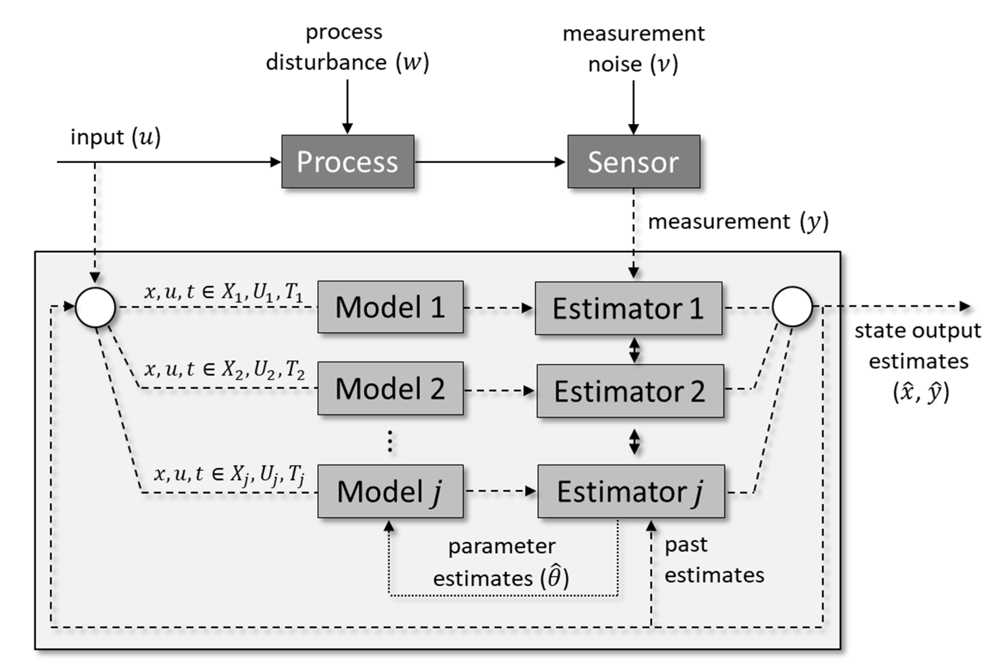
The state estimation based on the linearization of the process models, such as in the EKF method, may provide poor or even diverging estimates for highly nonlinear systems. A promising strategy to tackle this limitation is the use of hybrid state estimators, as illustrated in Figure 4. For instance, a hybrid MHE and EKF has already been designed for a process to produce a recombinant protein by E. coli bacteria [13]. In this proposed framework, the estimators operate hierarchically, with the EKF providing fast estimates between less frequent MHE calculations, which demand higher computational cost. MHE estimates, in turn, correct potential poor estimates from the EKF. Another hybrid approach has been proposed using the ELO and AO techniques [109]. In this study, the authors used a confidence function δ , varying from 0 to 1, to weigh the state estimators differently. In particular, the better the bioprocess model accuracy is, the closer δ is to 1, approximating the hybrid estimator to the ELO algorithm. At the other end, when the process kinetics is unknown, δ is close to 0 and the state estimator corresponds to the AO.
When model parameters depend on time, the performance of the state estimators may be hampered due potential plant-model mismatches. In such cases, it is possible to carry out the joint estimation of both bioprocess states and model parameters, as represented in Figure 4. Through this approach, the mathematical model is updated over time, reducing the model mismatch and hence improving the state estimate’s accuracy. This strategy has been proposed and tested for a variety of bioprocess case studies [106,110,111]. A simple approach to perform the joint estimation is to consider the parameters as extra states with no dynamics (i.e., constants), and define an augmented state vector x ˜ = [ x   θ ] T , according to Equation (9) [44,112]. Using this alternative formulation, the parameter estimation task is restated as a state estimation problem, which can thus be addressed using nonlinear state estimators.
d x ˜ d t = f ˜ ( x ˜ ,   u ) = [ f ( x , u , θ ) ;   0   ]
with x ( t 0 ) = x 0 and θ ( t 0 ) = θ 0 .
Finally, there are systems whose dynamics may not be fully described by single models throughout the process or operating conditions, as represented by Equation (8). In these cases, multiple (simple) models can be used, either in an on-off switching policy or combining them using fuzzy logic, for example, to guarantee a smooth transition between process models [52], as outlined in Figure 4. Then, state estimators may be implemented based on multiple process models, switching the models abruptly or smoothly according to specific ranges of system states, input variables, and/or process time. The commutation (on-off switching) between three specific growth models, valid under different ranges of substrate concentrations, was applied in reference [107]. The authors used the MHE to estimate the cell and substrate concentrations, as well as the specific growth rate, for a generic cultivation process. In [108], on the other hand, trust factors β , ranging from 0 to 1, were implemented to value gradually the contribution of output predictions from three process models to the MHE objective function. These trust factors, in turn, depend on the past and current model accuracy (i.e., distance between measured and predicted outputs) at a time instant t k , during a bioprocess operation to produce poly- β -hydroxybutyrate (PHB).
Overall, the aforementioned approaches (for hybrid state estimation, joint state and parameter estimation, and estimation based on multiple process models) are promising to overcome most of the limitations regarding bioprocess applications. However, there is no general solution that will apply to all biochemical processes. In other words, each system will demand specific strategies to deal with its particular challenges, possibly apart from the techniques already existing in the literature. This fact reinforces the need for the constant development of novel nonlinear state estimation strategies in the field of bioprocess monitoring.

3.5. Online Implementation

As state estimation is critical for online process control, one crucial challenge of online nonlinear state estimation is the reduction in computational time for implementation. Reduced-order models are commonly formulated as an attempt to problem complexity reduction [113,114,115]. More efficient sampling methods were also developed specifically for state estimation using the properties of Markov model approaches as well as parallelization [116,117]. Moreover, more advanced numerical optimization methods were proposed to allow the solution of MHE to converge more efficiently by employing sensitive-based strategies [118,119].
In many industrial applications, some measurements instantly arrive from hardware sensors, while other measurements are accompanied by a random time delay due to the requirements of offline lab procedures or the soft sensor’s computational time [120]. The combination of these measurement types often gives a more accurate state estimation for nonlinear processes, and data fusion techniques may be required for their integration [121]. Measurement fusion methods based on KF keep a time stamp on each fast measurement and update the estimations again after the delayed measurements are available [122,123]. Alternatively, the MHE can be reformulated offline according to different scenarios of delayed measurement arrivals, and an optimal procedure derived to select the appropriate formulation online to quickly update the state variables [124].
While traditional model predictive control (MPC) algorithms initialize with the state variables given by the state estimator, more advanced MPC algorithms also consider the uncertainty of the states to form more conservative constraints [125] or to guarantee a maximum chance of constraint violations [126,127]. However, more advanced methods for combining MPC and MHE are still lacking and thus could be a potentially fruitful area of research. In the next section, a case study is addressed to highlight some nonlinear state estimation challenges encountered during implementation.

4. Case Study Highlighting Nonlinear Estimation Implementation Challenges

4.1. Background

To highlight the performance and computational time challenges of nonlinear state estimation methods, a case study involving the implementation of EKF and MHE is performed considering the nonlinear case study from reference [128]. This case study consists of a batch reactor model considering the reaction mechanism shown below in Equations (10) and (11) and the corresponding system of differential equations in Equations (12)–(14).
A k 1 k 1 2 B
B k 2 C
d C a d t = k 1 C a + k 1 C b 2
d C b d t = 2 k 1 C a 2 k 1 C b 2 k 2 C b
d C c d t = k 2 C b
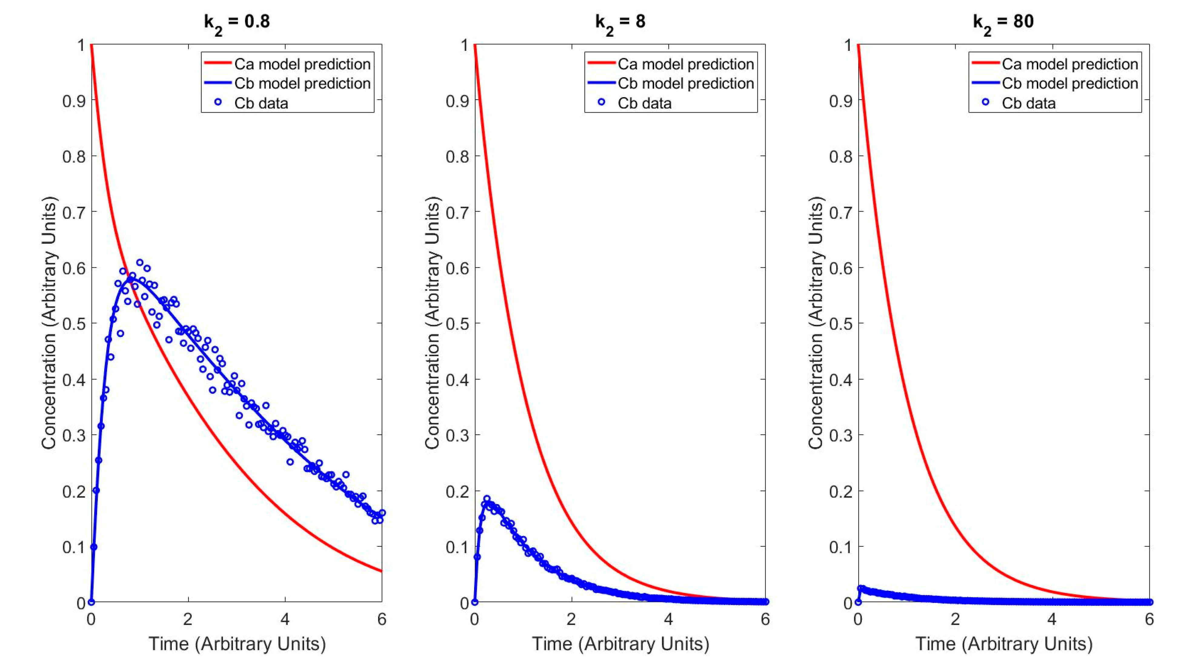
in which k1, k1, and k2 are the reaction kinetic parameters and Ca, Cb, and Cc are the concentrations and state variables. For all case studies performed, k1 and k−1 are fixed to a value of 1 with appropriate units, while k2 can change to either a value of 0.8, 8, or 80 with appropriate units. These k2 values are assumed to be the real k2 values and are used to generate the simulated data/measurements associated with the plant model. As component C does not influence the estimation implementations below, its concentration has not been included in the state-space model shown in Equation (15).
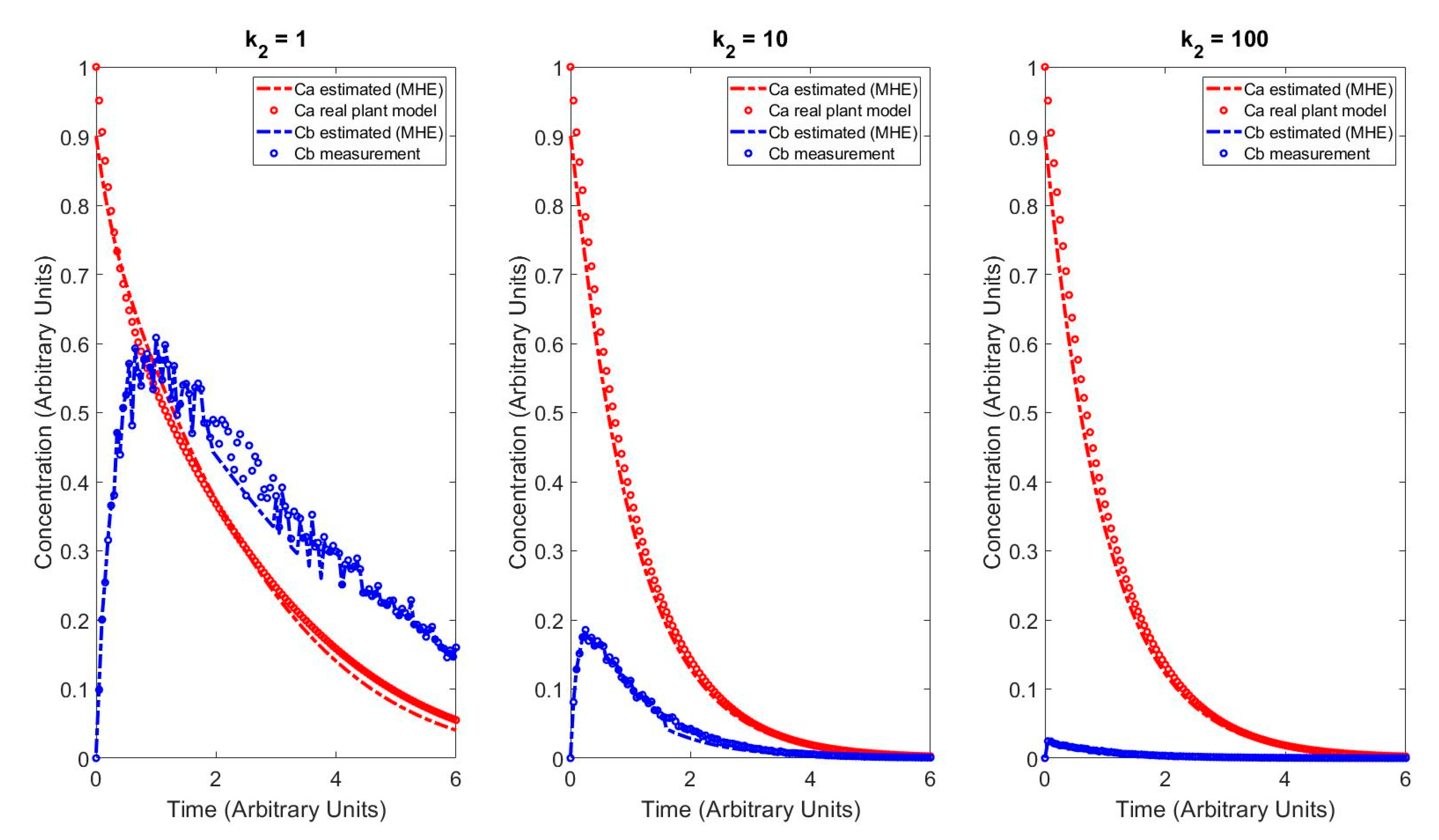
The system of differential equations above is integrated between 0 and 6 time units with a data point collected every 0.05 time units using the MATLAB ode15s function. As the value of k2 increases, the system becomes increasingly stiff, mandating the use of a stiff ODE solver. To generate noisy measurement data, the MATLAB function randn is used to apply a 5% normally distributed noise to component B concentrations considered as the only measurements used in the case study. For this case study, initial concentrations of components A and B are set to a value of 1 and 0 concentration units, respectively. The concentration profiles for the different k2 values are shown in Figure 5.
To increase the complexity of the estimation problem, the real k2 values are not used in the estimation model. Instead, a new set of k2 values known as the ideal k2 values (1, 10, and 100) are used to induce a plant-model mismatch. This mismatch is common in industrial settings where unmodeled disturbances such as catalyst deactivation or coking can occur over time and cause process models to deviate from the behavior happening in the real process. Furthermore, as the real state values of components A and B are known in this case study, the MSE calculation uses these values to characterize estimator performance.

4.2. EKF Results

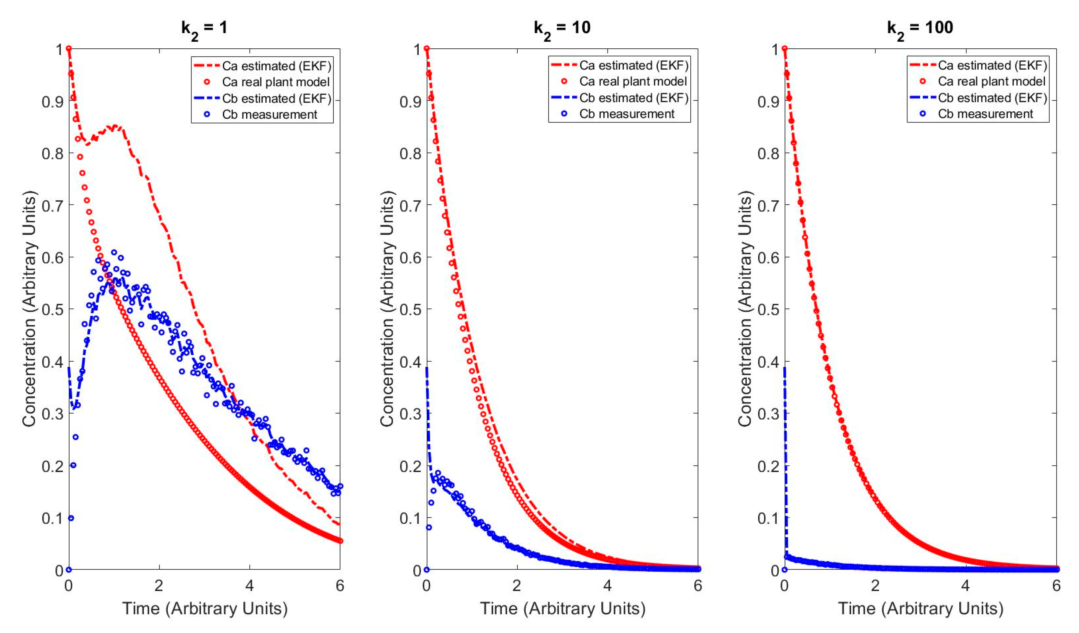
Using the simulated measurements and ideal k2 values, an EKF is applied to the reactor system employing a testing value of 0.001 for the diagonal elements of the process noise matrix (Q) of size 2 × 2 and a testing value of 0.0035 for the measurement noise matrix (R) of size 1 × 1. These values were chosen as most of the noise in the system is derived from the measurements, hence R is greater than Q. Additionally, approximations of the noise were used, as it mirrors how estimation is often conducted in industrial processes. It is also assumed that an accurate initial estimate of the concentration of state B is unavailable, providing an additional challenge to the implemented state estimator. Thus, the initial concentrations of component A and component B are assumed to be 1 and 0.5 concentration units, respectively. Additionally, the initial value of the covariance matrix (P-(0)) for the EKF is specified as a diagonal 2 × 2 matrix with diagonal elements of values of 0.001. Equations (15) and (16) display the symbolic linearized statespace model for this system. Figure 6 shows the EKF implementation results, considering each ideal k2 value.
A k = [ k 1 2 k 1 C b 2 k 1 k 2 4 k 1 C b ] k
C k = [ 0 ,   1 ]
The estimation results shown in Figure 6 are those taken after the correction step of the EKF. As a result, at time 0, the EKF generates an estimated concentration of B of approximately 0.38, which is between the poor initial guess of 0.5 and the measurement of 0. Figure 6 shows that when k2 has a value of 1, there is a large offset between the EKF estimates and the real plant values for the concentration of component A. This offset is the result of linearizing the nonlinear reactor model at the current iteration of the EKF and conducting the forecasting step using the linearized model. As the value of k2 increases, this offset becomes minimal due to a decrease in the linearization error of component A as reflected in the MSE values in Table 1. This decrease in the linearization error helps to reduce the offset between the nonlinear reactor model and the EKF model and ultimately lowers the MSE values. In terms of the estimation performance of component B, the EKF generates estimates that are mostly consistent with the measurement data and thus it does not appear to be impacted by this linearization error. The most significant offset for component B occurs during the first few estimation steps where only a poor initial value of the state is available. Although component A is not measured directly, the real plant data shown for this state serve as a way of gauging the performance of the EKF. To improve the EKF performance, the algorithm was modified to use ode15s to forecast the state estimate employing the original nonlinear differential equation model, while the linearized model was employed to update the covariance uncertainty. Figure 7 shows the results after making these modifications to the EKF forecasting step.
Figure 7 displays minimal offset between the model data and estimation results for the concentration of component A using a k2 value of 1 when nonlinear forecasting of the state is applied. Additionally, even the marginal offset present in the other k2 values is reduced when using nonlinear forecasting. In terms of the estimation of component B, the results remain largely unchanged as there is still offset during the first few estimation steps due to the poor initial guess. To quantify the improvement of the estimation performance, the MSE defined in Equation (7) is used to generate the values in Table 1 in terms of component A and component B using the true state value.
The values in Table 1 support the visual observations about the estimation performance. When nonlinear forecasting is applied in place of linear forecasting, there is a consistent decrease in the MSE for each of the k2 values shown. The most significant decrease is when there is a more than one order of magnitude decrease in the MSE when k2 has a value of 1. This result makes sense as nonlinear forecasting eliminates the linearization error associated with the EKF forecasting step. Although the EKF results improve when using this technique, it carries an increased computational time as discussed below in Section 4.4. A similar examination of linear vs. nonlinear forecasting was applied for the MHE implementation as well which is discussed in the next subsection.

4.3. MHE Results

When running the MHE implementations for this case study, the same covariances from the EKF and initial concentration estimates are applied. Additionally, as the MHE corresponds to a constrained optimization problem, both lower and upper bounds on the state variables are introduced. The lower bounds are specified such that all states have a concentration greater than or equal to 0. The upper bounds are specified to limit the concentrations to 2 arbitrary units. Initially, MATLAB’s fmincon solver using sqp was employed to solve the optimization problem with a horizon length (N) of 30 considering linear forecasting of the states where the objective function is the minimization of the MSE. For this specific case study, the arrival cost was not considered in the MHE formulation. The results for this case are shown in Figure 8.
The estimation results shown in Figure 8 are the final converged values of the MHE at the corresponding time instant. As a result, it can be seen that the MHE is able to overcome the poor initial concentration of component B by generally following the trajectory of the measurements to minimize the MSE. When using a horizon length of 30 and the fmincon subroutine, the estimation results of the MHE with linear forecasting are poor, as the offset between the model and estimation results for component A is significant for all k2 values. Beyond this offset, the estimated concentration of A experiences unexpected behavior as seen with the perturbations such as the one around 2 time units when k2 has a value of 1. As the value of k2 increases, the estimation performance appears to improve as the estimation results begin to converge to the real plant model with little offset. To attempt to improve the quality of these estimation results, nonlinear forecasting of the states in conjunction with different optimization solvers were explored. In particular, in addition to fmincon, the modified sequential quadratic programming (modSQP) algorithm from reference [129] was used to increase computational efficiency. The MHE results using modSQP and nonlinear forecasting are shown in Figure 9.
When using the modSQP optimization algorithm with an N of 30, more robust estimation results are able to be achieved in terms of several metrics. First, the offset of component A appears to be less pronounced as it is consistently decreasing at a smooth rate. Additionally, the estimation of component B is still acceptable, and the poor initial concentration estimate issue is overcome. Although the estimation performance of B may appear worse when compared to the linear case when k2 has a value of one, the MSE values in Table 2 do not support this conclusion.
Even though the decrease in MSE is less drastic than for the EKF implementation, switching to nonlinear forecasting presented smoother estimation curves with less MSE for all cases. To ensure that a horizon length of 30 was sufficiently large, a horizon length of 40 was applied to the nonlinear forecasting case. Ultimately, this had no effect as the estimation performance remained similar and the MSE values remained constant.

4.4. Computational Performance Analysis

One of the most important aspects of estimation that must be considered for online use is the balance between computational time and performance. Section 4.2 and Section 4.3 show that nonlinear forecasting generally produces more accurate estimation results, but do not highlight the increased computational time that occurred when changing the estimator formulation. For systems where rapid estimation is required, high computational times make the estimation become unsuitable and may require using less robust forms of estimation to maintain computational tractability. To compare the computational times of the case studies performed above, the stopwatch timer in MATLAB is used by calling the tic and toc functions. For reference, the computer used for all simulations is a Predator Helios 300 laptop equipped with a quad-core hyperthreaded i7-7700 HQ processor with a base clock of 2.81 GHz, running MATLAB R2020a. Table 3 depicts a comparison of the computational times of the two different EKF implementations tested.
The linear forecasting of Table 3 refers to the results in Figure 6 and the nonlinear forecasting refers to the results in Figure 7. The linear forecasting version of the EKF is an order of magnitude faster on average than the nonlinear forecasting version due to the absence of using ode15s to forecast the state estimate. Despite this order of magnitude difference, nonlinear forecasting can still be used by real processes, as all 120 estimation points were able to be solved in under 0.1 s while still providing excellent estimation results. On average, this method solves a single iteration of the EKF in under 0.001 s. Table 4 depicts the various MHE computational times for comparison against the EKF.
When examining Table 4, it is immediately evident that the MHE implementation is much slower than the EKF as the computational times are often three or more orders of magnitude greater than the EKF. Intuitively, this is reasonable, as a large optimization problem must be solved to generate the estimation results, unlike the EKF, which directly calculates the estimation forecast without optimization. To reduce the size of the optimization problem, the horizon length of the modSQP case was lowered to an N of 20 and yielded computational times approximately 57% less than the N of 30 case. However, there was an approximately 2% increase in the average MSE values when compared to the N = 30 case.
When attempting nonlinear forecasting using fmincon, the computational time increased by an order of magnitude when compared to the linear forecasting case as the complexity of the optimization problem increased in difficulty and the computational time per step was 46.2 s. This computational time value may make the fmincon-based MHE intractable depending on the sampling time rate. In contrast, the nonlinear forecasting-based modSQP MHE outperformed the estimation ability and computational time of the linear and nonlinear forecasting fmincon-based cases. Furthermore, for the k2 = 1 case, the average computational time to complete the estimation of one point was under 3 s. This relatively low computational time significantly improves the tractability of the MHE and makes it possible to implement in many real processes.
Therefore, by conducting this relatively simple nonlinear case study on a batch reactor model, the benefits of EKFs and MHEs were shown. Both techniques fail to generate desirable estimation results for the concentration of component A when using the linearized model to forecast the state estimate, despite having the lowest computational times. As a result, nonlinear forecasting should be employed to improve performance despite the increased computational time. This is of particular concern when using MHEs, as the computational time can approach intractability but can be mitigated through more efficient optimization techniques such as modSQP with an appropriate horizon length. Furthermore, based upon this case study, the MHE was shown to be more tolerant of a poor initial guess of the states, as it outperformed the EKF during the first steps of the estimation algorithm, as seen with their respective MSE values.

5. Opportunities and Future Trends

5.1. Development of Fast Optimization Techniques

As the case study highlighted, any MHE implementation will be highly dependent on the underlying optimization algorithm used in the state estimation formulation. Even though this paper is not a review of state-of-the-art optimization techniques, some of the most promising techniques for use in state estimation must be discussed. From the case study, it was shown that modSQP may be among the list of optimization algorithms that can be used in the next generation of state estimators.
The modSQP algorithm from [129] builds upon the existing SQP framework by utilizing a backtracking line search framework with a relaxed group of conditions to reach faster convergence. When applied as part of a model predictive control (MPC) implementation on a supercritical coal-fired power plant cycling problem, there was approximately a 25% decrease in computational time when compared to classical SQP MPC solvers used as a benchmark [129]. This feature was also demonstrated in the case study above when comparing the fmincon algorithm with sqp and the modSQP algorithm.
In addition to modSQP, other algorithms that have been successful in nonlinear MPC applications, such as IPOPT, and can likely reduce the computational time of the MHE optimization problem as well [130]. IPOPT is of interest as it is an open-source solver that has already been implemented on a case study of a low-density polyethylene (LDPE) tubular reactor as a solver for MHE and nonlinear model predictive control (NMPC) problems with success [119]. More specifically, this implementation of IPOPT was combined with an advanced-step framework which uses the current estimate for process control-associated predictions of both the states and measurements [118,119]. Alternatively, optimization algorithms for MHE such as the ones in the CasADi framework can be used for solving large-scale optimization problems [131].
Furthermore, as the number of cores on a CPU increases, the benefits of incorporating parallelization into optimization also increases. Modern CPUs are now available in a variety of multicore configurations including 8, 16, 32, and even 64 cores. Concurrently, performance of consumer grade GPUs has also rapidly increased in a similar manner in which new product launches offer top of the line performance with relatively low cost for performance. This decrease in cost and increase in performance creates an interesting opportunity to incorporate algorithms that can easily be parallelized, such as particle swarm optimization (PSO) or ant colony optimization into estimation applications, as they bring many unique benefits.
Global optimization techniques such as PSO disperse agents into the search space for an optimization problem and converge on the most optimum agent. Often in this convergence process, there is a chance that the global optimum can potentially be found, but these techniques have a history of solving complex problems at the cost of being very computationally heavy [132]. To overcome these limitations, GPU-based versions of PSO have been used since 2009 to decrease the computational time expense by orders of magnitudes [132]. Theoretically, as computer performance increases with new product launches, this decrease will likely continue further.
Additionally, it may be possible to combine optimizers such as PSO and SQP to improve the performance of optimization algorithms as seen in reference [133]. In this reference, PSO provides the initial guess of the SQP optimizer to improve the robustness of the gradient optimizer, while minimizing the computational time of running a full PSO algorithm. Although the specific application of this joint optimizer was dynamic real-time optimization (DRTO), similar hybrid optimizers could be formulated in conjunction with MHE to provide robust and fast results.

5.2. Heuristics for MHE Implementation

As the MHE is one of the state-of-the-art estimation techniques and is highly customizable, characterization of best practices or heuristics for MHE is sparse in the literature. For example, in many MHE publications, no guidelines are available for choosing horizon length, which may be crucial, as this directly affects the computational time for the implementation. The main rule of thumb reported corresponds to simply using a horizon length of twice the order of the system [31]. For more widespread adoption and implementation of MHE, a more comprehensive set of guidelines/heuristics should be available, as seen with chemical process design [134]. For example, in process design, there are often heuristics associated with economics, operation of process equipment, and safety considerations. Although these heuristics are not always directly applicable to all cases, in general they assist in a great number of cases.
If a set of MHE heuristics are developed, they could include topics such as optimization method selection, horizon length selection, objective function selection, etc. Characteristics such as model complexity, required computational time, available computational power, amount of system or measurement noise could guide the selection of the previously mentioned topics. It is likely that the hardest characteristic to define will be the model complexity. Tests could be developed to determine how well conditioned these models are, how nonlinear they are, or how computationally expensive they are to solve. Overall, the goal of these heuristics would be reducing the time to successfully implement an MHE. After successful implementation, case-specific tuning could be conducted to fine-tune performance.

5.3. Integration of Estimators with Commercial Software

As commercial chemical process simulators become more comprehensive through the incorporation of advanced control algorithms, dynamic optimization, and process monitoring tools, there is an excellent opportunity to develop state estimation tools in conjunction with such simulators. Although estimation may be available in some commercial simulators such as Aspen Dynamics, it is often limited to parameter estimation to improve dynamic models using a dataset. The features of Aspen DMC3 are limited to model conditioning, controller tuning, model adaptation, and Linear Programming tuning [135]. Previous controllers from AspenTech, such as the APC State-Space Controller, did incorporate a state estimation layer, but this was noted to come at the cost of having to develop a disturbance model and tune the filter. This additional task is often challenging to complete in industrial processes as process engineers often lack the formal control theory training that may be required [136].
Despite the limited industrial adoption of state estimation, Shell has historically incorporated these technologies in their products, such as SMOC and SMOCPro (Shell multivariable optimizing control) advanced controller. This technology employs disturbance models, model uncertainty, measurement noise, and state estimation via Kalman filtering [137,138]. More recently, Shell released a new generation of SMOC called PACE (Platform for Advanced Control and Estimation), which attempts to provide more flexibility in model structures [137].
The next generation of process simulators could follow Shell’s approach and introduce estimation into software. Many of these companies often offer products for online monitoring of real processes or that can connect to existing monitoring systems through OPC (Object Linking and Embedding for Process Control) servers. OPC is already an industrial standard and has been adopted by around 20 industries including pharmaceuticals [139]. As a result, the infrastructure already exists to combine and share data between process simulators, plant sensors, estimation algorithms, and advanced control systems towards the concept of Industry 4.0.

6. Conclusions

Today, state estimation is a very broad field of study and can be applied to almost any process including those outside of the chemical and biochemical process industries. Due to the vast size of the state estimation field, the primary goal in this work was to provide a general overview of the field with focus on chemical and biochemical processes. As Bayesian estimation methods are the most commonly applied and studied techniques, they were the primary focus of this work, with some discussion on elements of deterministic and hybrid methods. Bayesian estimation methods include recursive techniques such as the EKF, UKF, and PF along with optimization-based methods such as MHE.
As part of the general overview of the field, special attention was paid to some of the current challenges on nonlinear state estimation in bioprocess monitoring, uncertainty quantification, online implementation, covariance estimation, and time-scale multiplicity. Bioprocess monitoring provides many challenges to be addressed due to the lack of suitable measuring devices, highly complex nonlinear models (often black or grey box in nature), and time-varying parameters that require innovative estimation techniques.
Following the discussion on the current challenges, a case study was presented where EKF and MHE were applied to a nonlinear batch reactor model. Through the use of this case study, it was shown that linear forecasting of state estimates often results in poor estimation performance in nonlinear systems, despite conducting local linearization of the nonlinear model before forecasting. However, it was shown that with nonlinear forecasting improved estimation performance can be achieved. Additionally, the case study also examined the computational time of EKF- and MHE-based estimation implementations and noted that MHE was often three to four orders of magnitude more computationally expensive than the EKF methods. Furthermore, it was noted that for MHE estimation, special attention needs to be paid to the optimizer selection, as this directly affects the computational time and robustness of the estimation results. Finally, a brief discussion on the opportunities and future trends of state estimation was included where optimizer selection was emphasized.
Even though the focus of this paper was on chemical and biochemical processes, industries such as navigation, automotive control, aviation, etc., can benefit from the development of state estimation for chemical processes. We envision a growing reliance on estimation in the future as the Internet of Things, big data, and cloud computing grow in size and increase the access to raw data from sensors. Today, almost everyone is reliant on state estimation in some form or another. For example, today most people carry around a GPS-equipped smartphone which heavily relies on estimation to provide access to location services. As this reliance on state estimation increases, it will likely promote unique and additional opportunities for research in the future.

Author Contributions

This work was a collaborative effort amongst all authors. R.A., G.C., and S.D., wrote parts of the manuscript. R.A. performed the case study overseen by F.V.L. All authors assisted in editing the paper and contributed to the structure of this project and provided critical references. All authors have read and agreed to the published version of the manuscript.

Funding

The authors acknowledge the financial support from West Virginia University, in particular the Statler Fellowship for supporting R.A. PhD studies.

Conflicts of Interest

The authors declare no conflict of interest.

References

  1. Mohd Ali, J.; Ha Hoang, N.; Hussain, M.A.; Dochain, D. Review and classification of recent observers applied in chemical process systems. Comput. Chem. Eng. 2015, 76, 27–41. [Google Scholar] [CrossRef] [Green Version]
  2. Seborg, D.E.; Edgar, T.F.; Mellichamp, D.A.; Doyle, F.J. Process Dynamics and Control, 4th ed.; John Wiley & Sons Inc.: Hoboken, NJ, USA, 2017. [Google Scholar]
  3. Mesbah, A.; Huesman, A.E.M.; Kramer, H.J.M.; Van den Hof, P.M.J. A comparison of nonlinear observers for output feedback model-based control of seeded batch crystallization processes. J. Process Control 2011, 21, 652–666. [Google Scholar] [CrossRef]
  4. Lima, F.V.; Rajamani, M.R.; Soderstrom, T.A.; Rawlings, J.B. Covariance and State Estimation of Weakly Observable Systems: Application to Polymerization Processes. IEEE Trans. Control Syst. Technol. 2013, 21, 1249–1257. [Google Scholar] [CrossRef]
  5. Rincón, F.D.; Le Roux, G.A.C.; Lima, F.V. The Autocovariance Least-Squares Method for Batch Processes: Application to Experimental Chemical Systems. Ind. Eng. Chem. Res. 2014, 53, 18005–18015. [Google Scholar] [CrossRef]
  6. Rincón, F.D.; Esposito, M.; de Araújo, P.H.H.; Lima, F.V.; Le Roux, G.A.C. Robust Calorimetric Estimation of Semi-Continuous and Batch Emulsion Polymerization Systems with Covariance Estimation. Macromol. React. Eng. 2014, 8, 456–466. [Google Scholar] [CrossRef]
  7. Yin, X.; Liu, J. Distributed moving horizon state estimation of two-time-scale nonlinear systems. Automatica 2017, 79, 152–161. [Google Scholar] [CrossRef]
  8. López-Negrete, R.; Biegler, L. A Moving Horizon Estimator for processes with multi-rate measurements: A Nonlinear Programming sensitivity approach. J. Process Control 2012, 65, 4548–4556. [Google Scholar] [CrossRef]
  9. Rawlings, J.B.; Mayne, D.Q.; Diehl, M.M. State Estimation. In Model Predictive Control: Theory, Computation, and Design; Nob Hill Publishing: Santa Barbara, CA, USA, 2019; pp. 265–369. [Google Scholar]
  10. Varshney, D.; Bhushan, M.; Patwardhan, S.C. Robust State Estimation and Parameter Estimation for Linear and Nonlinear Direct Feed-through Systems with Correlated Disturbances. Ind. Eng. Chem. Res. 2019, 58, 11532–11552. [Google Scholar] [CrossRef]
  11. Raïssi, T.; Ramdani, N.; Candau, Y. Bounded error moving horizon state estimator for non-linear continuous-time systems: Application to a bioprocess system. J. Process Control 2005, 15, 537–545. [Google Scholar] [CrossRef]
  12. Wang, J.; Zhao, L.; Yu, T. On-line Estimation in Fed-batch Fermentation Process Using State Space Model and Unscented Kalman Filter. Chin. J. Chem. Eng. 2010, 18, 258–264. [Google Scholar] [CrossRef]
  13. Campani, G.; Ribeiro, M.P.A.; Zangirolami, T.C.; Lima, F.V. A hierarchical state estimation and control framework for monitoring and dissolved oxygen regulation in bioprocesses. Bioprocess Biosyst. Eng. 2019, 42, 1467–1481. [Google Scholar] [CrossRef] [PubMed]
  14. Furlong, V.B.; Corrêa, L.J.; Lima, F.V.; Giordano, R.C.; Ribeiro, M.P.A. Estimation of Biomass Enzymatic Hydrolysis State in Stirred Tank Reactor through Moving Horizon Algorithms with Fixed and Dynamic Fuzzy Weights. Processes 2020, 8, 407. [Google Scholar] [CrossRef] [Green Version]
  15. Lima, F.V.; Rawlings, J.B. Nonlinear stochastic modeling to improve state estimation in process monitoring and control. AIChE J. 2011, 57, 996–1007. [Google Scholar] [CrossRef]
  16. Afshari, H.H.; Gadsden, S.A.; Habibi, S. Gaussian filters for parameter and state estimation: A general review of theory and recent trends. Signal Process. 2017, 135, 218–238. [Google Scholar] [CrossRef]
  17. Rawlings, J.B.; Bakshi, B.R. Particle filtering and moving horizon estimation. Comput. Chem. Eng. 2006, 30, 1529–1541. [Google Scholar] [CrossRef]
  18. Rawlings, J.B.; Ji, L. Optimization-based state estimation: Current status and some new results. J. Process Control 2012, 22, 1439–1444. [Google Scholar] [CrossRef]
  19. Patwardhan, S.C.; Narasimhan, S.; Jagadeesan, P.; Gopaluni, B.; Shah, S.L. Nonlinear Bayesian state estimation: A review of recent developments. Control Eng. Pract. 2012, 20, 933–953. [Google Scholar] [CrossRef]
  20. Li, T.; Su, J.; Liu, W.; Corchado, J.M. Approximate Gaussian conjugacy: Parametric recursive filtering under nonlinearity, multimodality, uncertainty, and constraint, and beyond. Front. Inf. Technol. Electron. Eng. 2017, 18, 1913–1939. [Google Scholar] [CrossRef]
  21. Bayes, T. LII. An essay towards solving a problem in the doctrine of chances. By the late Rev. Mr. Bayes, F.R.S. communicated by Mr. Price, in a letter to John Canton, A.M.F.R.S. Philos. Trans. R. Soc. Lond. 1763, 53, 370–418. [Google Scholar]
  22. Gauss, C.F. Theory of the Motion of the Heavenly Bodies: Moving about the Sun in Conic Sections: A Translation of Theoria Motus; Dover: Mineola, NY, USA, 2004. [Google Scholar]
  23. Fisher, R.A. On an absolute criterion for fitting frequency curves. Messenger Math. 1912, 41, 155–160. [Google Scholar]
  24. Kolmogorov, A.N. Interpolation and Extrapolation of Stationary Sequences. Ser. Math. 1941, 5, 3–14. [Google Scholar]
  25. Wiener, N. Extrapolation, Interpolation, and Smoothing of Stationary Time Series with Engineering Application; MIT Press: Cambridge, MA, USA, 1964. [Google Scholar]
  26. Kalman, R.E. A New Approach to Linear Filtering and Prediction Problems. J. Basic Eng. 1960, 82, 35–45. [Google Scholar] [CrossRef] [Green Version]
  27. Julier, S.J.; Uhlmann, J.K. Unscented Filtering and Nonlinear Estimation. Proc. IEEE 2004, 92, 401–422. [Google Scholar] [CrossRef] [Green Version]
  28. Kolås, S.; Foss, B.A.; Schei, T.S. Constrained nonlinear state estimation based on the UKF approach. Comput. Chem. Eng. 2009, 33, 1386–1401. [Google Scholar] [CrossRef]
  29. Prakash, J.; Patwardhan, S.; Shah, S. Constrained Nonlinear State Estimation Using Ensemble Kalman Filters. Ind. Eng. Chem. Res. 2010, 49, 2242–2253. [Google Scholar] [CrossRef]
  30. Ungarala, S.; Dolence, E.; Li, K. Constrained extended Kalman filter for nonlinear state estimation. IFAC Proc. Vol. 2007, 40, 63–68. [Google Scholar] [CrossRef]
  31. Rao, C.V.; Rawlings, J.B. Constrained process monitoring: Moving-horizon approach. AIChE J. 2002, 48, 97–109. [Google Scholar] [CrossRef]
  32. Arulampalam, M.S.; Maskell, S.; Gordon, N.; Clapp, T. A tutorial on particle filters for online nonlinear/non-Gaussian Bayesian tracking. IEEE Trans. Signal Process. 2002, 50, 174–188. [Google Scholar] [CrossRef] [Green Version]
  33. Chen, T.; Morris, J.; Martin, E. Particle filters for state and parameter estimation in batch processes. J. Process Control 2005, 15, 665–673. [Google Scholar] [CrossRef] [Green Version]
  34. Imtiaz, S.A.; Roy, K.; Huang, B.; Shah, S.L.; Jampana, P. Estimation of States of Nonlinear Systems using a Particle Filter. In Proceedings of the 2006 IEEE International Conference on Industrial Technology, Mumbai, India, 15–17 December 2006; pp. 2432–2437. [Google Scholar]
  35. Shenoy, A.V.; Prakash, J.; Prasad, V.; Shah, S.L.; McAuley, K.B. Practical issues in state estimation using particle filters: Case studies with polymer reactors. J. Process Control 2013, 23, 120–131. [Google Scholar] [CrossRef]
  36. Rajamani, M.R.; Rawlings, J.B. Improved State Estimation using a Combination of Moving Horizon Estimator and Particle Filters. In Proceedings of the 2007 American Control Conference, New York, NY, USA, 9–13 July 2007; pp. 4443–4444. [Google Scholar]
  37. Markana, A.; Padhiyar, N.; Moudgalya, K. Multi-criterion control of a bioprocess in fed-batch reactor using EKF based economic model predictive control. Chem. Eng. Res. Des. 2018, 136, 282–294. [Google Scholar] [CrossRef]
  38. Vachhani, P.; Narasimhan, S.; Rengaswamy, R. Robust and reliable estimation via Unscented Recursive Nonlinear Dynamic Data Reconciliation. J. Process Control 2006, 16, 1075–1086. [Google Scholar] [CrossRef]
  39. Lang, L.; Chen, W.; Bakshi, B.R.; Goel, P.K.; Ungarala, S. Bayesian estimation via sequential Monte Carlo sampling—Constrained dynamic systems. Automatica 2007, 43, 1615–1622. [Google Scholar] [CrossRef] [Green Version]
  40. Chitralekha, S.B.; Prakash, J.; Raghavan, H.; Gopaluni, R.B.; Shah, S.L. A comparison of simultaneous state and parameter estimation schemes for a continuous fermentor reactor. J. Process Control 2010, 20, 934–943. [Google Scholar] [CrossRef]
  41. Abdollahi, J.; Dubljevic, S. Lipid production optimization and optimal control of heterotrophic microalgae fed-batch bioreactor. Chem. Eng. Sci. 2012, 84, 619–627. [Google Scholar] [CrossRef]
  42. Ellis, M.; Zhang, J.; Liu, J.; Christofides, P.D. Robust moving horizon estimation based output feedback economic model predictive control. Syst. Control Lett. 2014, 68, 101–109. [Google Scholar] [CrossRef]
  43. Bastin, D.; Dochain, G. State and Paramater Estimation with Known Yield Coefficients. In On-line Estimation and Adaptive Control of Bioreactors; Elsevier: Amsterdam, The Netherlands, 1990; pp. 101–200. [Google Scholar]
  44. Dochain, D. State and parameter estimation in chemical and biochemical processes: A tutorial. J. Process Control 2003, 13, 801–818. [Google Scholar] [CrossRef]
  45. Méndez-Acosta, H.O.; Palacios-Ruiz, B.; Alcaraz-González, V.; Steyer, J.-P.; González-Álvarez, V.; Latrille, E. Robust Control of Volatile Fatty Acids in Anaerobic Digestion Processes. Ind. Eng. Chem. Res. 2008, 47, 7715–7720. [Google Scholar] [CrossRef]
  46. Dochain, D. State observers for tubular reactors with unknown kinetics. J. Process Control 2000, 10, 259–268. [Google Scholar] [CrossRef]
  47. Dochain, D.; Couenne, F.; Jallut, C. Enthalpy based modelling and design of asymptotic observers for chemical reactors. Int. J. Control 2009, 82, 1389–1403. [Google Scholar] [CrossRef]
  48. Hadj-Sadok, M.Z.; Gouzé, J.L. Estimation of uncertain models of activated sludge processes with interval observers. J. Process Control 2001, 11, 299–310. [Google Scholar] [CrossRef]
  49. Aziz, N.; Hussain, M.A.; Mujtaba, I.M. Performance of different types of controllers in tracking optimal temperature profiles in batch reactors. Comput. Chem. Eng. 2000, 24, 1069–1075. [Google Scholar] [CrossRef]
  50. Kadlec, P.; Gabrys, B.; Strandt, S. Data-driven Soft Sensors in the process industry. Comput. Chem. Eng. 2009, 33, 795–814. [Google Scholar] [CrossRef] [Green Version]
  51. Horta, A.C.L.; da Silva, A.J.; Sargo, C.R.; Gonçalves, V.M.; Zangirolami, T.C.; de Campos Giordano, R. Robust artificial intelligence tool for automatic start-up of the supplementary medium feeding in recombinant E. coli cultivations. Bioprocess Biosyst. Eng. 2011, 34, 891–901. [Google Scholar] [CrossRef]
  52. Furlong, V.B.; Corrêa, L.J.; Giordano, R.C.; Ribeiro, M.P.A. Fuzzy-Enhanced Modeling of Lignocellulosic Biomass Enzymatic Saccharification. Energies 2019, 12, 2110. [Google Scholar] [CrossRef] [Green Version]
  53. Porru, G.; Aragonese, C.; Baratti, R.; Servida, A. Monitoring of a CO oxidation reactor through a grey model-based EKF observer. Chem. Eng. Sci. 2000, 55, 331–338. [Google Scholar] [CrossRef] [Green Version]
  54. Prakash, J.; Senthil, R. Design of observer based nonlinear model predictive controller for a continuous stirred tank reactor. J. Process Control 2008, 18, 504–514. [Google Scholar] [CrossRef]
  55. Vafamand, N.; Arefi, M.M.; Khayatian, A. Nonlinear system identification based on Takagi-Sugeno fuzzy modeling and unscented Kalman filter. ISA Trans. 2018, 74, 134–143. [Google Scholar] [CrossRef]
  56. Fang, H.; de Callafon, R.A.; Cortés, J. Simultaneous input and state estimation for nonlinear systems with applications to flow field estimation. Automatica 2013, 49, 2805–2812. [Google Scholar] [CrossRef]
  57. Tulsyan, A.; Huang, B.; Bhushan Gopaluni, R.; Fraser Forbes, J. On simultaneous on-line state and parameter estimation in non-linear state-space models. J. Process Control 2013, 23, 516–526. [Google Scholar] [CrossRef]
  58. Nelles, O. Nonlinear System Identification; Springer: Berlin/Heidelberg, Germany, 2001. [Google Scholar]
  59. Ogata, K. Control Systems Analysis in State Space. In Modern Control Engineering; Prentice Hall: Upper Saddle River, NJ, USA, 2010. [Google Scholar]
  60. Muske, K.R.; Edgar, T.F. Nonlinear State Estimation. In Nonlinear Process Control; Henson, M.A., Seborg, D.E., Eds.; Prentice Hall PTR: Upper Saddle River, NJ, USA, 1997. [Google Scholar]
  61. Reinschke, K. Multivariable Control a Graph-Theoretic Approach, 1st ed.; Springer: Berlin/Heidelberg, Germany, 1988. [Google Scholar]
  62. Sueur, C.; Dauphin-Tanguy, G. Bond-graph approach for structural analysis of MIMO linear systems. J. Frankl. Inst. 1991, 1, 55–70. [Google Scholar] [CrossRef]
  63. Spivey, B.J.; Hedengren, J.D.; Edgar, T.F. Constrained Nonlinear Estimation for Industrial Process Fouling. Ind. Eng. Chem. Res. 2010, 49, 7824–7831. [Google Scholar] [CrossRef]
  64. Heffes, H. The Effect of Erroneous Models on the Kalman Filter Response. IEEE Trans. Autom. Control 1966, 11, 541–543. [Google Scholar] [CrossRef]
  65. Nishimura, T. Error Bounds of Continuous Kalman Filters and the Application to Orbit Determination Problems. IEEE Trans. Autom. Control 1967, 12, 268–275. [Google Scholar] [CrossRef]
  66. Duník, J.; Kost, O.; Straka, O.; Blasch, E. State and Measurement Noise in Positioning and Tracking: Covariance Matrices Estimation and Gaussian Assessment. In Proceedings of the IEEE/ION Position, Location and Navigation Symposium (PLANS), Monterey, CA, USA, 23–26 April 2018. [Google Scholar]
  67. Odelson, B.; Rajamani, M.; Rawlings, J. A New Autocovariance Least-Squares Method for Estimating Noise Covariances. Available online: https://sites.engineering.ucsb.edu/~jbraw/jbrweb-archives/tech-reports/twmcc-2003-04.pdf (accessed on 14 November 2020).
  68. Rajamani, M.; Rawlings, J. Estimation of the disturbance structure from data using semidefinite programming and optimal weighting. Automatica 2009, 45, 142–148. [Google Scholar] [CrossRef]
  69. Duník, J.; Kost, O.; Straka, O.; Blasch, E. Covariance Estimation and Gaussinity Assessment for State and Measurement Noise. J. Guid. Control Dyn. 2020, 43, 132–139. [Google Scholar] [CrossRef] [Green Version]
  70. Duník, J.; Straka, O.; Kost, O.; Havlík, J. Noise covariance matrices in state-space models: A survey and comparison of estimation methods—Part 1. Int. J. Adapt. Control Signal Process. 2017, 31, 1505–1543. [Google Scholar] [CrossRef]
  71. Simon, D. Optimal State Estimation: Kalman, H Infinity, and Nonlinear Approaches, 1st ed.; John Wiley & Sons: Hoboken, NJ, USA, 2006. [Google Scholar]
  72. Gharamti, M.E.; Hoteit, I. Complex step-based low-rank extended Kalman filtering for state-parameter estimation in subsurface transport models. J. Hydrol. 2014, 509, 588–600. [Google Scholar] [CrossRef]
  73. Lü, H.; Yu, Z.; Drake, S.; Hao, Z.; Sudicky, E. Dual state-parameter estimation of root zone soil moisture by optimal parameter estimation and extended Kalman filter data assimilation. Adv. Water Resour. 2011, 34, 395–406. [Google Scholar] [CrossRef]
  74. Van der Merwe, R.; Wan, E.A. The square-root unscented Kalman filter for state and parameter-estimation. In Proceedings of the 2001 IEEE International Conference on Acoustics, Speech, and Signal Processing, Salt Lake City, UT, USA, 7–11 May 2001. [Google Scholar]
  75. Moradkhani, H.; Sorooshian, S.; Gupta, H.V.; Houser, P.R. Dual state–parameter estimation of hydrological models using ensemble Kalman filter. Adv. Water Resour. 2005, 28, 135–147. [Google Scholar] [CrossRef] [Green Version]
  76. Varshney, D.; Bhushan, M.; Patwardhan, S.C. State and parameter estimation using extended Kitanidis Kalman filter. J. Process Control 2019, 76, 98–111. [Google Scholar] [CrossRef]
  77. Kühl, P.; Diehl, M.; Kraus, T.; Schlöder, J.P.; Bock, H.G. A real-time algorithm for moving horizon state and parameter estimation. Comput. Chem. Eng. 2011, 35, 71–83. [Google Scholar] [CrossRef]
  78. Valluru, J.; Lakhmani, P.; Patwardhan, S.C.; Biegler, L.T. Development of moving window state and parameter estimators under maximum likelihood and Bayesian frameworks. J. Process Control 2017, 60, 48–67. [Google Scholar] [CrossRef]
  79. Wiener, N. The homogeneous chaos. Am. J. Math. 1938, 60, 897–936. [Google Scholar] [CrossRef]
  80. Xiu, D.; Karniadakis, G.E. The Wiener–Askey polynomial chaos for stochastic differential equations. SIAM J. Sci. Comput. 2002, 24, 619–644. [Google Scholar] [CrossRef]
  81. Bavdekar, V.; Mesbah, A. A Polynomial Chaos-Based Nonlinear Bayesian Approach for Estimating State and Parameter Probability Distribution Functions. In Proceedings of the 2016 American Control Conference, Boston, MA, USA, 6–8 July 2016; pp. 2047–2052. [Google Scholar]
  82. Dutta, P.; Bhattacharya, R. Nonlinear Estimation of Hypersonic State Trajectories in Bayesian Framework with Polynomial Chaos. J. Guid. Control Dyn. 2010, 33, 1765–1778. [Google Scholar] [CrossRef]
  83. Li, J.; Xiu, D. A generalized polynomial chaos based ensemble Kalman filter with high accuracy. J. Comput. Phys. 2009, 228, 5454–5469. [Google Scholar] [CrossRef]
  84. Blanchard, E.; Sandu, A.; Sandu, C. A Polynomial Chaos-Based Kalman Filter Approach for Parameter Estimation of Mechanical Systems. J. Dyn. Syst. Meas. Control 2010, 132, 061404. [Google Scholar] [CrossRef]
  85. Alspach, D.; Sorenson, H. Nonlinear Bayesian estimation using Gaussian sum approximations. IEEE Trans. Autom. Control 1972, 17, 439–448. [Google Scholar] [CrossRef]
  86. Ito, K.; Xiong, K. Gaussian filters for nonlinear filtering problems. IEEE Trans. Autom. Control 2000, 45, 910–927. [Google Scholar] [CrossRef] [Green Version]
  87. Terejanu, G.; Singla, P.; Singh, T.; Scott, P.D. Uncertainty Propagation for Nonlinear Dynamic Systems Using Gaussian Mixture Models. J. Guid. Control Dyn. 2008, 31, 1623–1633. [Google Scholar] [CrossRef]
  88. Gauvain, J.; Lee, C. Maximum a posteriori estimation for multivariate Gaussian mixture observations of Markov chains. IEEE Trans. Speech Audio Process. 1994, 2, 291–298. [Google Scholar] [CrossRef]
  89. Risken, H.; Frank, T. The Fokker-Planck Equation, 2nd ed.; Springer: Berlin/Heidelberg, Germany, 1996. [Google Scholar]
  90. Muscolino, G.; Ricciardi, G.; Vasta, M. Stationary and non-stationary probability density function for non-linear oscillators. Int. J. Non-Linear Mech. 1997, 32, 1051–1064. [Google Scholar] [CrossRef]
  91. Paola, M.; Sofi, A. Approximate solution of the Fokker–Planck–Kolmogorov equation. Probabilistic Eng. Mech. 2002, 17, 369–384. [Google Scholar] [CrossRef]
  92. Kumar, M.; Singla, P.; Chakravorty, S.; Junkins, J. The Partition of Unity Finite Element Approach to the Stationary Fokker-Planck Equation. In Proceedings of the AIAA/AAS Astrodynamics Specialist Conference and Exhibit, Keystone, CO, USA, 21–24 August 2006. [Google Scholar] [CrossRef] [Green Version]
  93. Becerra, V.; Roberts, P.; Griffiths, G. Dynamic data reconciliation for a class of nonlinear differential-algebraic equation models using the extended Kalman filter. IFAC Proc. Vol. 1999, 32, 5961–5966. [Google Scholar] [CrossRef]
  94. Becerra, V.; Roberts, P.; Griffiths, G. Applying the extended Kalman filter to systems described by nonlinear differential-algebraic equations. Control Eng. Pract. 2001, 9, 267–281. [Google Scholar] [CrossRef]
  95. Mandela, R.; Rengaswamy, R.; Narasimhan, S. Nonlinear State Estimation of Differential Equations. IFAC Proc. Vol. 2009, 42, 792–797. [Google Scholar] [CrossRef]
  96. Mandela, R.; Rengaswamy, R.; Narasimhan, S.; Sridhar, L. Recursive state estimation techniques for nonlinear differential algebraic systems. Chem. Eng. Sci. 2010, 65, 4548–4556. [Google Scholar] [CrossRef]
  97. Kraus, T.; Kühl, P.; Wirsching, L.; Bock, H.; Diehl, M. A Moving Horizon State Estimation algorithm applied to the Tennessee Eastman Benchmark Process. In Proceedings of the 2006 IEEE International Conference on Multisensor Fusion and Integration for Intelligent Systems, Heidelberg, Germany, 3–6 September 2006. [Google Scholar]
  98. Shuler, M.L.; Kargi, F.; DeLisa, M.P. Bioprocess Engineering: Basic Concepts, 3rd ed.; Prentice Hall: Boston, MA, USA, 2017. [Google Scholar]
  99. FDA. Guidance for Industry PAT—A Framework for Innovative Pharmaceutical Development, Manufacturing, and Quality Assurance; Food and Drug Administration: Rockville, MD, USA, 2004; p. 16.
  100. Simon, L.L.; Pataki, H.; Marosi, G.; Meemken, F.; Hungerbühler, K.; Baiker, A.; Tummala, S.; Glennon, B.; Kuentz, M.; Steele, G.; et al. Assessment of Recent Process Analytical Technology (PAT) Trends: A Multiauthor Review. Org. Process Res. Dev. 2015, 19, 3–62. [Google Scholar] [CrossRef]
  101. Zhao, L.; Fu, H.-Y.; Zhou, W.; Hu, W.-S. Advances in process monitoring tools for cell culture bioprocesses. Eng. Life Sci. 2015, 15, 459–468. [Google Scholar] [CrossRef]
  102. Pörtner, R.; Platas Barradas, O.; Frahm, B.; Hass, V.C. Advanced Process and Control Strategies for Bioreactors. In Current Developments in Biotechnology and Bioengineering; Elsevier: Amsterdam, The Netherlands, 2017; pp. 463–493. [Google Scholar]
  103. Komives, C.; Parker, R.S. Bioreactor state estimation and control. Curr. Opin. Biotechnol. 2003, 14, 468–474. [Google Scholar] [CrossRef] [PubMed]
  104. Venkateswarlu, C. Advances in monitoring and state estimation of bioreactors. J. Sci. Ind. Res. 2004, 63, 491–498. [Google Scholar]
  105. Cuthbertson, A.B.; Rodman, A.D.; Diab, S.; Gerogiorgis, D.I. Dynamic Modelling and Optimisation of the Batch Enzymatic Synthesis of Amoxicillin. Processes 2019, 7, 318. [Google Scholar] [CrossRef] [Green Version]
  106. Jabarivelisdeh, B.; Carius, L.; Findeisen, R.; Waldherr, S. Adaptive predictive control of bioprocesses with constraint-based modeling and estimation. Comput. Chem. Eng. 2020, 135, 106744. [Google Scholar] [CrossRef]
  107. Valdes-Gonzalez, H.; Flaus, J.-M. State estimation in a bioprocess described by a hybrid model. In Proceedings of the 2001 IEEE International Symposium on Intelligent Control (ISIC ’01) (Cat. No.01CH37206), Mexico City, Mexico, 5–7 September 2001; pp. 132–137. [Google Scholar]
  108. Morabito, B.; Kienle, A.; Findeisen, R.; Carius, L. Multi-mode Model Predictive Control and Estimation for Uncertain Biotechnological Processes. IFAC-PapersOnLine 2019, 52, 709–714. [Google Scholar] [CrossRef]
  109. Hulhoven, X.; Wouwer, A.V.; Bogaerts, P. Hybrid extended Luenberger-asymptotic observer for bioprocess state estimation. Chem. Eng. Sci. 2006, 61, 7151–7160. [Google Scholar] [CrossRef]
  110. Bogaerts, P.; Hanus, R. On-line state estimation of bioprocesses with full horizon observers. Math. Comput. Simul. 2001, 56, 425–441. [Google Scholar] [CrossRef]
  111. Simutis, R.; Lübbert, A. Bioreactor control improves bioprocess performance. Biotechnol. J. 2015, 10, 1115–1130. [Google Scholar] [CrossRef]
  112. Murtuza Baker, S.; Poskar, C.H.; Schreiber, F.; Junker, B.H. An improved constraint filtering technique for inferring hidden states and parameters of a biological model. Bioinformatics 2013, 29, 1052–1059. [Google Scholar] [CrossRef] [Green Version]
  113. Hyland, D.; Bernstein, D. The optimal projection equations for model reduction and the relationships among the methods of Wilson, Skelton, and Moore. IEEE Trans. Autom. Control 1985, 30, 1201–1211. [Google Scholar] [CrossRef] [Green Version]
  114. Bernstein, D.S.; Haddad, W.M. Steady-state Kalman filtering with an H∞ error bound. Syst. Control Lett. 1989, 12, 847–852. [Google Scholar] [CrossRef]
  115. Xu, S.; Chen, T. Reduced-order H/sub/spl infin//filtering for stochastic systems. IEEE Trans. Signal Process. 2002, 50, 2998–3007. [Google Scholar]
  116. Doucet, A.; Gordon, N.J.; Krishnamurthy, V. Particle filters for state estimation of jump Markov linear systems. IEEE Trans. Signal Process. 2001, 49, 613–624. [Google Scholar] [CrossRef]
  117. Tong, G.; Fang, Z.; Xu, X. A Particle Swarm Optimized Particle Filter for Nonlinear System State Estimation. In Proceedings of the 2006 IEEE International Conference on Evolutionary Computation, Vancouver, BC, Canada, 16–21 July 2006. [Google Scholar]
  118. Thierry, D.; Nicholson, B.; Biegler, L. A General Framework for Sensitivity-Based Optimal Control and State Estimation. Comput. Aided Chem. Eng. 2018, 44, 787–792. [Google Scholar]
  119. Zavala, V.M.; Biegler, L.T. Nonlinear programming strategies for state estimation and model predictive control. In Nonlinear Model Predictive Control, 1st ed.; Magni, L., Raimondo, D.M., Allogöwer, F., Eds.; Springer: Berlin, Germany, 2009; Volume 384, pp. 419–432. [Google Scholar]
  120. Fatehi, A.; Huang, B. Kalman filtering approach to multi-rate information fusion in the presence of irregular sampling rate and variable measurement delay. J. Process Control 2017, 53, 15–25. [Google Scholar] [CrossRef]
  121. Gopalakrishnan, A.; Kaisare, N.; Narasimhan, S. Incorporating delayed and infrequent measurements in Extended Kalman Filter based nonlinear state estimation. J. Process Control 2011, 21, 119–129. [Google Scholar] [CrossRef]
  122. Mahmoud, M.S.; Emzir, M.F. State estimation with asynchronous multi-rate multi-smart sensors. Inf. Sci. 2012, 196, 15–27. [Google Scholar] [CrossRef]
  123. Zhao, L.; Wang, R.; Wang, J.; Yu, T.; Su, A. Nonlinear state estimation with delayed measurements using data fusion technique and cubature Kalman filter for chemical processes. Chem. Eng. Res. Des. 2019, 141, 502–515. [Google Scholar] [CrossRef]
  124. Gu, Y.; Chou, Y.; Liu, J.; Ji, Y. Moving horizon estimation for multirate systems with time-varying time-delays. J. Frankl. Inst. 2019, 356, 2325–2345. [Google Scholar] [CrossRef]
  125. Mayne, D.Q.; Kerrigan, E.C.; Wyk, E.J.; Falugi, P. Tube-based robust nonlinear model predictive control. Int. J. Robust Nonlinear Control 2011, 21, 1341–1353. [Google Scholar] [CrossRef]
  126. Lorenzen, M.; Allgöwer, F.; Cannon, M. Adaptive Model Predictive Control with Robust Constraint Satisfaction. IFAC-PapersOnLine 2017, 50, 3313–3318. [Google Scholar] [CrossRef]
  127. Paulson, J.; Mesbah, A. An efficient method for stochastic optimal control with joint chance constraints for nonlinear systems. Int. J. Robust Nonlinear Control 2017, 29, 5017–5037. [Google Scholar] [CrossRef]
  128. Pantea, C.; Gupta, A.; Rawlings, J.; Craciun, G. The QSSA in Chemical Kinetics: As Taught and as Practiced. In Discrete and Topological Models in Molecular Biology; Natural Computing Series; Springer: Berlin/Heidelberg, Germany, 2013; pp. 419–442. [Google Scholar]
  129. He, X.; Lima, F.V. A modified SQP-based model predictive control algorithm: Application to supercritical coal-fired power plant cycling. Ind. Eng. Chem. Res. 2020, 59, 15671–15681. [Google Scholar] [CrossRef]
  130. Wächter, A.; Biegler, L. On the implementation of an interior-point filter line-search algorithm for large-scale nonlinear programming. Math. Program. 2006, 106, 25–57. [Google Scholar] [CrossRef]
  131. Andersson, J.; Gills, J.; Horn, G.; Rawlings, J.; Diehl, M. CasADi: A software framework for nonlinear optimization and optimal control. Math. Program. Comput. 2018, 11, 1–36. [Google Scholar] [CrossRef]
  132. Zhou, Y.; Tan, Y. GPU-based Parallel Particle Sawm Optimization. In Proceedings of the 2009 IEEE Congress on Evolutionary Computation, Trondheim, Norway, 18–21 May 2009; pp. 1493–1500. [Google Scholar]
  133. Kim, R.; Lima, F.V. A Tchebycheff-based multi-objective combined with a PSO-SQP dynamic real-time optimization framework for cycling energy systems. Chem. Eng. Res. Des. 2020, 156, 180–194. [Google Scholar] [CrossRef]
  134. Turton, R.; Shaeiwitz, J.; Bhattacharyya, D.; Whiting, W. Utilizin Experience-Based Principles to Confirm the Suitability of a Process Design. In Analysis, Synthesis and Design of Chemical Processes, 5th ed.; Pearson: Boston, MA, USA, 2018; pp. 347–368. [Google Scholar]
  135. Golightly, R. The Aspen DMC3TM Difference. Available online: https://www.aspentech.com/-/media/AspenTech/Home/Resources/White%20Papers/PDFs/11-8885-WP-DMC3%20Difference (accessed on 13 November 2020).
  136. Froisy, J. Model predictive control—Building a bridge between theory and practice. Comput. Chem. Eng. 2006, 30, 1426–1435. [Google Scholar] [CrossRef]
  137. Amrit, R.; Canney, W.; Carrette, P.; Linn, R.; Martinez, A.; Singh, A.; Skrovanek, T.; Valiquette, J.; Williamson, J.; Zhou, J.; et al. Platform for Advanced Control and Estimation (PACE): Shell’s and Yokogawa’s Next Generation Advanced Process Control Technology. IFAC-PapersOnLine. 2015, 48, 1–5. [Google Scholar] [CrossRef]
  138. Mayne, D.; Rawlings, J.; Rao, C.; Scokaert, P. Constrained model predictive control: Stability and optimality. Automatica 2000, 36, 789–814. [Google Scholar] [CrossRef]
  139. Latif, H.; Shao, G.; Starly, B. Integrating a Dynamic Simulator and Advanced Process Control using the OPC-UA Standard. Procedia Manuf. 2019, 34, 813–819. [Google Scholar] [CrossRef]
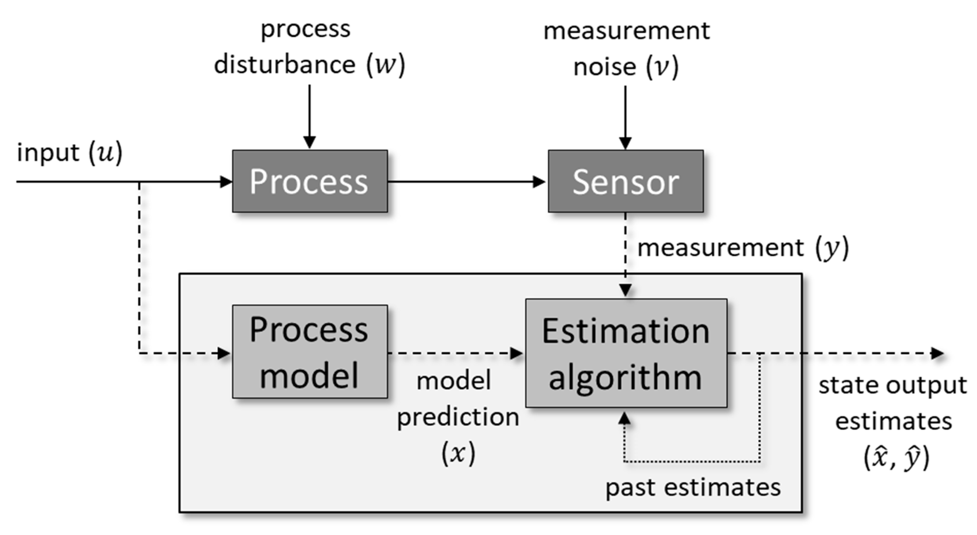
Figure 1. Schematic diagram of state estimation. The solid lines indicate system connections, while the dashed and dotted lines refer to information signals.
Processes 08 01462 g001
Figure 2. General classification of the main nonlinear state estimators used for chemical and biochemical systems. Representative estimators are depicted in the brackets under each subgroup.
Processes 08 01462 g002
Figure 3. General approach for the design of nonlinear state estimators.
Processes 08 01462 g003
Figure 4. Schematic diagram of estimation procedure including hybrid state estimation, joint parameter and state estimation, and estimation based on multiple process models. The solid lines indicate system connections, and the dashed and dotted lines refer to information signals.
Processes 08 01462 g004
Figure 5. Concentration profiles considering a variety of k2 values. The solid lines correspond to the plant model results from ode15s and the markers correspond to the measurement/simulated plant data.
Processes 08 01462 g005
Figure 6. Extended Kalman filter (EKF) implementation profiles considering a variety of ideal k2 values. The markers correspond to the simulated measurements or the real state values using the real k2 values, and the dashed lines correspond to the EKF estimates.
Processes 08 01462 g006
Figure 7. EKF implementation profiles using nonlinear forecasting considering a variety of ideal k2 values. The markers correspond to the simulated measurements or the real state values using the real k2 values and the dashed lines correspond to the EKF estimates.
Processes 08 01462 g007
Figure 8. Moving horizon estimation (MHE) profiles considering a variety of k2 values using linear forecasting and an N of 30. The markers correspond to the simulated measurements or the real state values using the real k2 values and the dashed lines correspond to the MHE estimates.
Processes 08 01462 g008
Figure 9. MHE profiles considering a variety of k2 values and an N of 30 using nonlinear forecasting and modSQP. The markers correspond to the simulated measurements or the real state values using the real k2 values, and the dashed lines correspond to the MHE implementation.
Processes 08 01462 g009
Table 1. Mean squared error (MSE) values for EKF variations.
k2 = 1k2 = 10k2 = 100
EKF, Linear Forecasting0.04400.002040.00125
EKF, Nonlinear Forecasting0.002560.001610.00125
Table 2. MSE values for MHE variations.
k2 = 1k2 = 10k2 = 100
MHE, Linear Forecasting0.007010.002770.00408
MHE, Nonlinear Forecasting0.001250.0007320.000839
Table 3. EKF computational times.
Trialk2 = 1k2 = 10k2 = 100Average Time Per Step
Linear Forecasting0.0181 s0.00816 s0.00572 s8.88∙10−5 s
Nonlinear Forecasting0.0642 s0.0676 s0.0778 s5.82∙10−4 s
Table 4. MHE computational times for different formulations.
Trialk2 = 1k2 = 10k2 = 100Average Time Per Step
n = 30, linear forecasting, fmincon610 s400 s399 s5.22 s
n = 30, nonlinear forecasting, fmincon3966 s4499 s4027 s46.2 s
n = 30, nonlinear forecasting, modSQP458 s172 s159 s2.92 s
n = 20, nonlinear forecasting, modSQP193 s80.8 s67.7 s1.26 s
Publisher’s Note: MDPI stays neutral with regard to jurisdictional claims in published maps and institutional affiliations.