1. Introduction
The last decades have witnessed great research progress in the field of fault detection and diagnosis using multivariate statistical process control techniques (MSPC). Among all MSPC techniques, traditional methods such as principal component analysis (PCA) [
1,
2,
3], principal component regression (PCR) [
4,
5], and partial least squares (PLS) [
6,
7] are perhaps the most popular. One of the limitations of traditional methods is that they are designed for Gaussian processes, while it is commonly acknowledged that industrial systems are generally non-Gaussian or even nonlinear. To deal with non-Gaussian or nonlinear processes, different kinds of independent component analysis (ICA) [
8,
9,
10,
11,
12,
13] based approaches have been proposed. The basic idea of ICA based approaches is to decompose the process data into independent components so that non-Gaussian and Gaussian components can be separated. By considering statistical independence of the extracted components, ICA involves higher order statistics of process data implicitly.
More recently, He and Wang [
14] suggested the use of statistical pattern analysis to monitor non-Gaussian batch processes and further extended it to the monitoring of continuous process. Unlike ICA based approaches, the SPA framework considers high order statistics of process data explicitly. It examines change in the variance-covariance (e.g., mean, variance, cross-correlation, autocorrelation etc.) as well other higher order statistics of the process data using a window based approach. These statistics are called statistical patterns (SPs). It is assumed that the considered SPs followed a Gaussian distribution so that PCA could be applied to determine whether there was a faulty condition. The advantages of SPA are obvious: it does not employ a data preprocessing step and by using various statistics of process variables, it can capture different process characteristics. However, since the SPA framework uses the statistics of process variables explicitly, a large number of statistics may be required to fully capture the process characteristics; hence, significantly increasing the scale and dimensionality of the problem. As a result, it is not suitable for the monitoring of complex multivariate processes because the monitoring sensitivity will be reduced by considering a large number of statistics.
In this work, we proposed monitoring the statistics of process variables with the same order using empirical likelihood [
15] to increase sensitivity and reduce the dimensionality of the SP matrix. Empirical likelihood is a nonparametric method used to construct confidence regions for finite-dimensional parameters [
16]. It is widely used to test, for example, symmetry about zero, change in distribution, independence, etc. [
17]. By considering the change in statistics with the same order, it is possible to know which kind of characteristics have changed in the process variables and hence reveal more information about the potential process faults.
The rest of the paper is organized as follows. The next section presents the basic idea of statistical pattern analysis based monitoring strategy. In
Section 3, empirical likelihood is introduced.
Section 4 proposes the improved SPA monitoring strategy, followed by a demonstration of the application of the methodology in
Section 5. Finally, a concluding summary is given in
Section 6.
2. Statistical Pattern Analysis Based Monitoring Strategy
The rationale of SPA based monitoring strategy is that statistics of process variables under abnormal conditions will be different from those under normal operational conditions. Hence, process faults can be detected by considering the statistics of process variables instead of the process variables themselves. The SPA based monitoring strategy consists of two steps: construction of statistical patterns, and quantification of dissimilarity. A statistical pattern is a statistic calculated from a consecutive set of process measurements through a window based strategy. These statistics include the mean value, variance, and skewness, which capture the characteristics of individual variables; correlation coefficient that captures the interactions among variables as well as autocorrelation and cross-correlation that captures the process dynamics. In other words, statistics that capture different kinds of characteristics of complex multivariate processes can be considered.
Generation of statistical patterns can be achieved by a moving window approach. Denote the process measurement at time instance
k by
,where
m is the number of process variables, and a window of process measurements can be generated as
where
is the window length and
is the most recent measurement of
. The statistical patterns are generated from Equation (1). The authors in [
14,
15] considered four sets of process statistics
In Equation (2),
relates to variable means, or first order statistics, which are calculated from Equation (1) as
where
M1 is the number of first order statistics. On the other hand,
represents the second order statistics including variance
, correlation
, autocorrelation
, and cross correlation
. These statistics can be computed as
where
d is the time lag between variables and
M2 is the number of second order statistics.
Finally,
represents the third order statistics like skewness
and
relates to the fourth order statistics like kurtosis
, which can be calculated as
where
M3 and
M4 are the numbers of the third and fourth order statistics. Statistics higher than four orders can also be considered, however, for the sake of simplicity, only the above statistics were considered here. With different statistics calculated, a statistical pattern vector can be obtained by putting together all the statistical patterns in a row vector. The row vector reflects the statistical properties of process variables at the window from
k-w + 1 to
k, so that an SP matrix can be obtained as
, where
M is the number of SPs and
.
By inspecting the statistical pattern vector at different windows using principal component analysis, the fault can be detected. The SPA monitoring framework considers the statistics quantifying the non-Gaussianity and nonlinearity of process data; it is capable of monitoring non-Gaussian and nonlinear processes. However, for complex multivariate processes, there is a large number of variables. Using the SPA framework may lead to consideration of too many statistics. For example, for a six variable process, considering the statistics listed from Equations (3)–(9) may involve six mean values, 21 variance and covariance components, six skewness values, and six kurtosis values. There was a total of 39 statistics, not to mention other terms like autocorrelation and cross correlation terms. To simplify the monitoring task, we used empirical likelihood to monitor changes in statistics with the same order, so that only four monitoring statistics were needed.
3. Empirical Likelihood
Empirical likelihood is a nonparametric approach used to define confidence regions for omnibus hypothesis testing. As a nonparametric approach, it is distribution free; the error of the confidence region obtained by empirical likelihood is Bartlett correctable [
16].
As pointed out in
Section 2, as there were too many statistics considered in the original SPA framework, we considered monitoring the change in statistics with the same order using empirical likelihood. Assume we have
N normal data samples and the statistical pattern matrix
has been calculated from the original data. As a new data sample
arrives, a moving window approach can be used to obtain the SP vector by considering the statistics of
, denoted as
. Take the first order statistic, for example, to monitor the change in first order statistics
, another moving window approach should be considered (i.e.,
). Denote the probability density function of
as
, and the following hypothesis test can be constructed
where
is the mean value of
and
is the length of the sliding window. If the alternative hypothesis holds, then the new data sample
is a faulty sample with a fault in the first order statistics.
With the hypothesis test in Equation (10), it is possible to detect fault in the first order statistics. However, the hypothesis test cannot be used only when the confidence limit is available, which can be obtained by maximizing the following empirical likelihood function
subject to the following constraints
where
is the probability of
. The maximum can be reached if and only if
for all
, so that the null hypothesis
holds. Otherwise,
holds and faults in the first order statistic can be observed.
To obtain the probability
, consider the following log-likelihood ratio
subject to the constraints in Equation (12).
Using the Lagrange multiplier, we have
Differentiating Equation (14) and setting it to be zero, the probability
can be obtained as
where
is the solution of the following equation
Equation (16) can be solved using gradient search as follows
where
and
are the values of
λ at the
t-th and (
t + 1)-th iteration of the gradient search;
is the learning rate;
is the derivative of
at
and can be obtained as
Combining Equations (17) and (18), the updating formula of
in the gradient search can be obtained as follows.
Once is determined, the probability and hence the log-likelihood ratio can be computed from Equations (13) and (15). Similar procedures can be employed for second order statistics and higher order statistics .
4. Process Monitoring Strategy Based on Improved Statistical Pattern Analysis
With the statistical patterns obtained in
Section 2, process monitoring can be performed by constructing monitoring plots using the empirical likelihood method in
Section 3. Assume a statistical pattern matrix
has already been obtained using the
N training data samples by a moving window approach (with the window length of
w). When a new data sample
arrives, another statistical pattern vector
can be obtained based on
and its previous
s-1 samples. The statistical pattern vector is then augmented with the previous
w-1 vectors to form a new statistical pattern matrix
. Empirical likelihood can then be performed between
and
. Here, we performed a total of four empirical likelihood tests on the SP matrices, corresponding to the first, second, third, and fourth order statistical patterns. With the log-likelihood ratios estimated, fault detection can then be performed.
The process monitoring strategy can be divided into an offline training stage and an online monitoring stage, which are illustrated in
Section 4.1 and
Section 4.2.
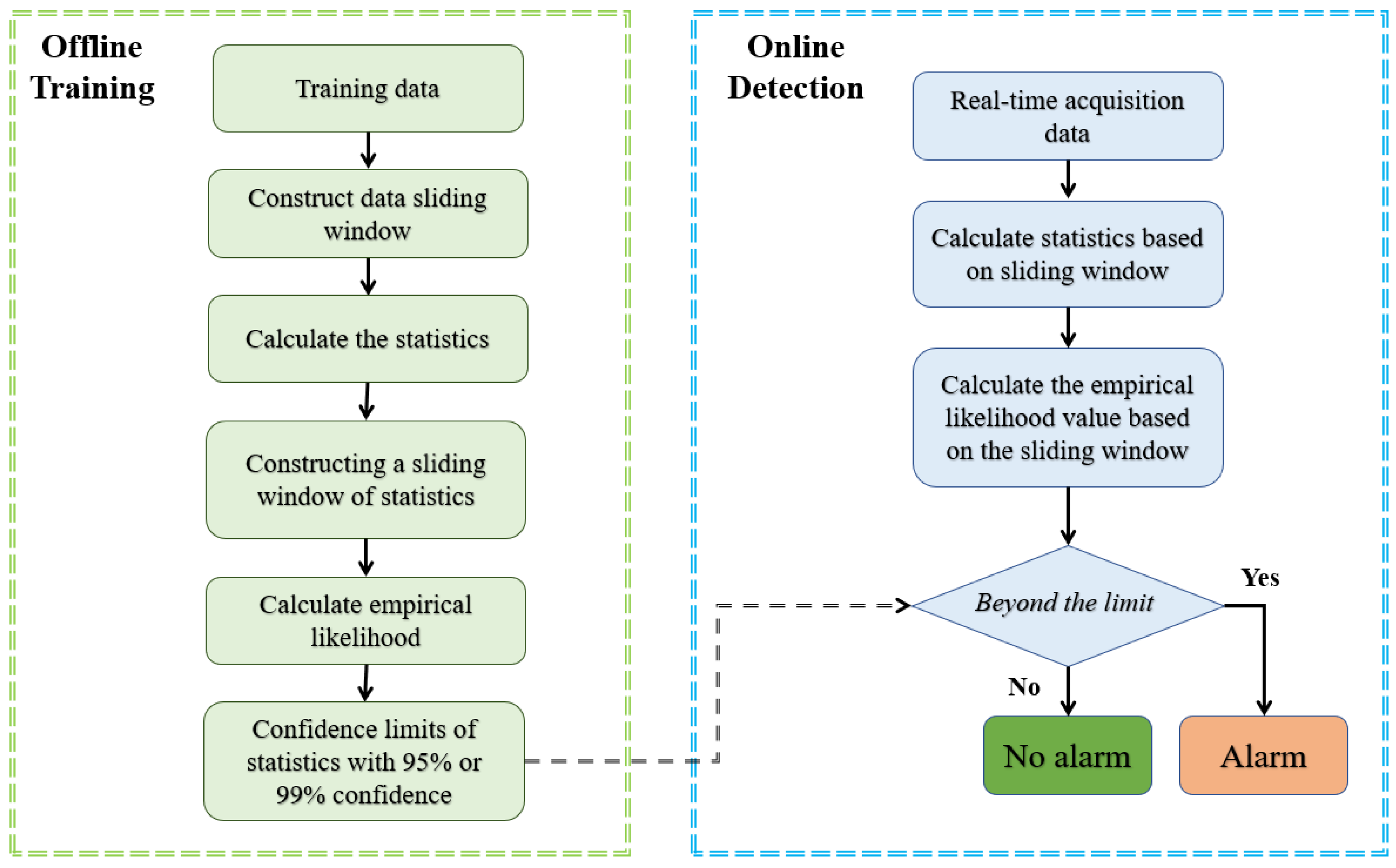
Figure 1 shows the flowchart of the process monitoring strategy.
4.1. Offline Training Stage
The offline training stage can be summarized as follows.
Step 1: Collect N normal samples under normal conditions, set the lengths of the two sliding windows as s and w.
Step 2: Perform the first moving window processing based on the normal samples, construct groups of measurement matrices using Equation (1). Calculate the first order, second order, third order, and fourth order statistics from the samples in each sub-window to form the statistical pattern matrix based on Equations (3)–(9).
Step 3: Divide the statistical patter matrix into two parts with equal length, and . Let , use as the base SP matrix, and divide into a series of submatrices with the length of s using the moving window approach.
Step 4: Perform empirical likelihood tests between the four sets of statistics in and those in the series of submatrices of . Since and contain SPs corresponding to the first-, second-, third-, and fourth-order statistics, a total of four sets of log-likelihood ratios, defined as , can be obtained. For each set of log-likelihood ratios, determine its confidence limit using methods like kernel density estimation, or simply using the 95% or 99% quantiles as the confidence limits.
4.2. Online Monitoring Stage
Once the confidence limits for the four SPs have been obtained, it is now possible to perform online monitoring on new data samples. For a new sample
, a new SP vector can be obtained as
can be estimated. Based on
and its previous
w-1 SP vectors, four SP matrices corresponding to the first-, second-, third-, and fourth-order statistics can be obtained, following the moving window approach discussed in
Section 3.
Empirical likelihood tests are then performed between the SP matrices corresponding to the new data sample and those in to get the log-likelihood ratios of , which are used as monitoring statistics. If either of the four log-likelihood ratios exceed the confidence limit, a fault is detected and an alarm is triggered.
The advantages of the proposed empirical likelihood based monitoring strategy are double folded. In addition to reducing the size of the problem, it can provide a better understanding of the process changes. For example, if a change in first-order statistical patterns is detected, then the mean values of the variable is abnormal. If the second-order statistical patterns change, the fault causes an anomaly in variances or correlation structure. Third-order statistical patterns such as skewness are used to measure the degree of skewness of the data. If an anomaly occurs, it indicates that the process variables do not follow Gaussian distribution. Fourth-order statistical patterns such as kurtosis can be used to test the nonlinearity of the process data. If there is a violation, it indicates that the process becomes nonlinear.
5. Application Study
This section examines the performance of the improved statistical pattern analysis method on fault detection of the Tennessee Eastman (TE) process. The TE process is a simulation of a chemical process that has been widely used to test the performance of fault diagnosis and process control technologies. It was initially published by the Tennessee Eastman company [
18] for academic research. The process contains 12 manipulated variables and 41 measured variables. There are four main operation units: reactor, condenser, compressor, and product separator. Four reactants labeled as Feed A, Feed C, Feed D, and Feed E were fed into the process and two products were produced. In addition, the process defines different constraints, process disturbances, and operating modes.
Figure 2 presents a simplified diagram of the process.
Following the recommendation of [
19], 22 measured variables and 11 manipulated variables were selected for process monitoring, as listed in
Table 1.
For the purpose of fault detection, a normal dataset containing 500 samples was generated. A typical fault (i.e., fault 5) was considered and tested, which contained 960 samples. Fault 5 involves a step change in the condenser cooling water inlet temperature, which was introduced after the 160th sample. During the fault, the cooling ability was influenced and hence a change in the vapor–liquid ratio of the input flow separator was observed.
For the purpose of fault detection, both window lengths of
w,
s were set as 50. Statistical pattern matrices involving mean value, variance, skewness, and kurtosis were constructed. Empirical likelihood was then used to construct the monitoring statistic for each of the pattern matrices and four statistics
were then constructed. The monitoring results are shown in
Figure 3.
In
Figure 3,
is the monitoring statistic for the first order statistics (mean value);
is for the second order statistics (variance);
is for the third order statistics (skewness); and
is for the fourth order statistics (kurtosis). It should be noted that due to the introduction of two moving windows, the length of the monitoring statistics was reduced from 960 to 860, indicating that if correctly detected, the fault will cause violations in the statistics of
Figure 3 after the 60th sample. From
Figure 3, it can be seen that some violations could be observed for
and
after the 60th sample. At a later time, the fault becomes more severe and a significant number of violations were observed for
, especially after the 250th sample. Hence, the fault was successfully detected by the statistic
, which indicates that the fault influences both the mean values of process variables, resulting in a certain degree of nonlinearity in the process data. It should also be noted that the monitoring statistic
becomes a constant in the later stage. This was due to the fact that at the later stage, the impact of the fault on the mean values becomes so severe that the estimated log-likelihood values become very great. Hence, a cut-off line was introduced.
On the other hand, the second order statistic and third order statistic could hardly detect any violation, indicating no change happened in the second and third order statistical patterns. In addition, fault 5 also influenced the fourth order statistic , indicating that the fault introduced some kinds of process nonlinearity. This can be explained as step change in the cooling water inlet temperature may influence the process setpoint and introduce process nonlinearity.
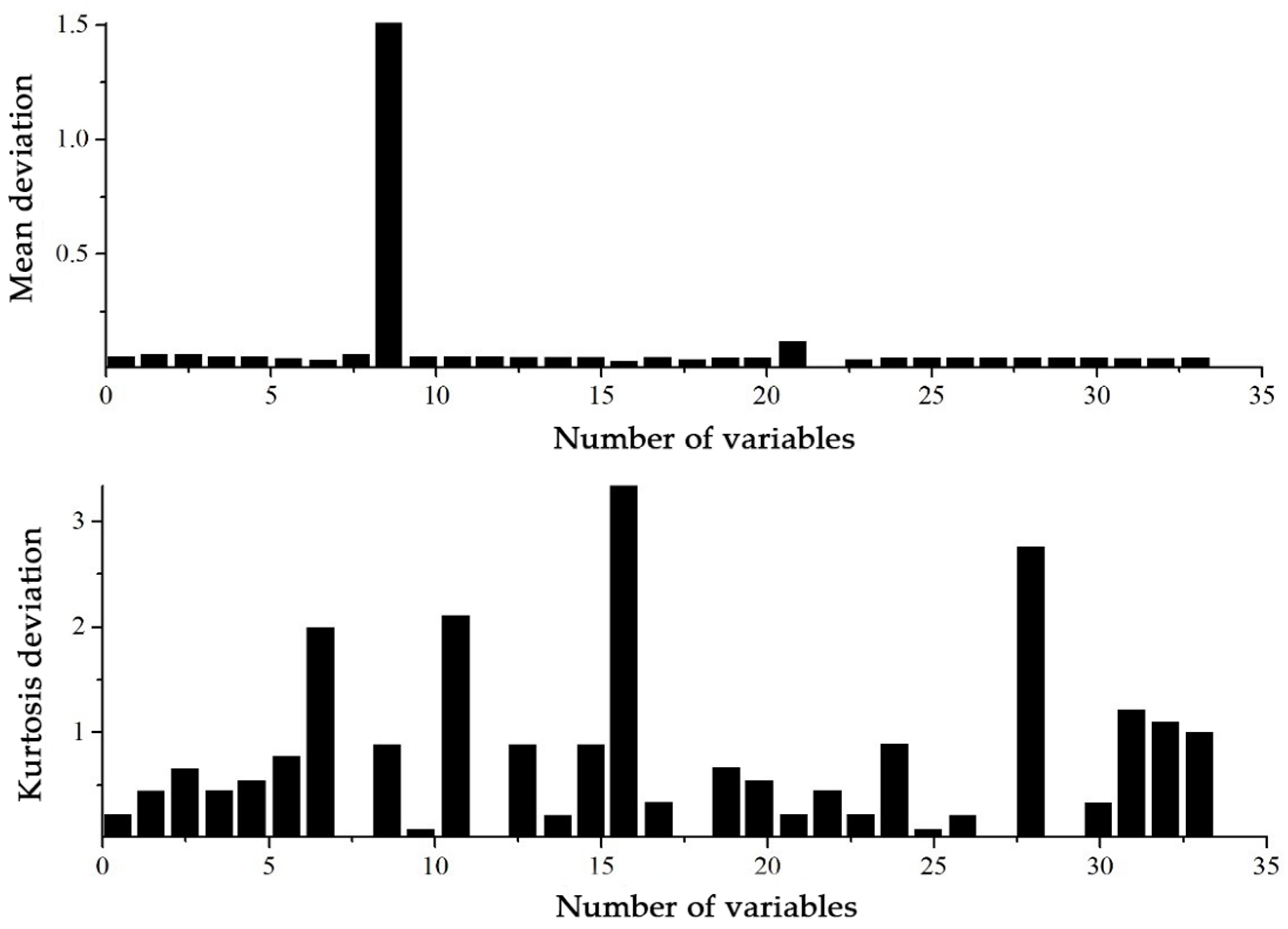
After the fault is detected, it is important to isolate which variable is affected by the fault. Since few violations are detected in the skewness and kurtosis in this monitoring model, they are not considered in fault isolation. The deviations of mean values and kurtoses between normal and faulty samples for the 33 variables are shown in
Figure 4. For a clearer inspection,
Table 2 presents the variables with the most significant deviations in mean values and kurtoses due to the fault.
It can be seen from
Table 2 that the variables
x9,
x21,
x16,
x11,
x7,
x31,
x32, and
x33 had significant deviations. This can be explained as fault 5 involves a step change in the inlet temperature of the condenser cooling water, so the reactor cooling water outlet temperature
x21 of the cooling water of the separator will be affected. In addition, since the gas flow is cooled by the condenser and fed into the separator, it will cause the product separator temperature
x11, the separator cooling water flow
x33, and the separator pot liquid flow
x29.The separated steam is recycled into the reactor through the compressor, causing changes in the reactor temperature
x9, reactor cooling water flow rate
x32, and reactor cooling water outlet temperature
x21.
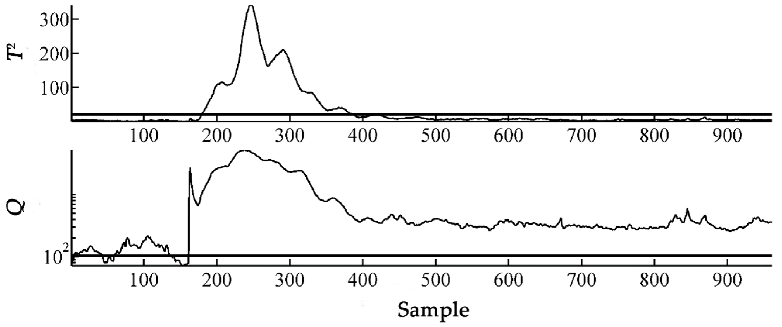
For comparison, the SPA monitoring method proposed in [
14] was also tested. In SPA monitoring, four sets of statistical patterns (i.e., mean, variance, skewness and kurtosis) are considered and a SP matrix with 132 statistical patterns was obtained by setting the window length as 50. It was found that retaining eight principal components was sufficient to capture 95.3% variance. Hence, the number of principal components was set as eight. The monitoring results are shown in
Figure 5. It can be seen from
Figure 5 that the fault was successfully detected by the T
2 and Q statistics of SPA monitoring, however, it did not reveal any information on fault type. Furthermore, the SP matrix included a total of 132 patterns, which may cause difficulties in subsequent fault isolation.
It can be seen from
Figure 3 and
Figure 5 that the improved statistical pattern analysis based on empirical likelihood not only successfully detected the fault, but could also learn the type of fault and the specific information of faulty variables while reducing the scale of the monitoring model, leading to a simple and parsimonious model. Although the SPA monitoring method in [
14] also successfully detected the step fault, it could not provide any further fault information. Therefore, the improved statistical pattern analysis based on empirical likelihood is more effective and comprehensive than the SPA monitoring method. One additional issue about the proposed method is that it involves a solution of an optimization problem for each online sample, resulting in greater computation load. In this case study, the average computation time for the empirical likelihood method was 0.0325s on a personal computer with the configuration of an Intel (R) Core (TM) i7-6700 CPU @ 3.40 GHz, RAM: 8.0 GB, which is acceptable for online application. Hence, the computation load does not pose a serious problem for our method.


