Abstract
In this paper we have considered a staggered cavity. It is equipped with purely viscous fluid. The physical design is controlled through mathematical formulation in terms of both the equation of continuity and equation of momentum along with boundary constraints. To be more specific, the Navier-Stokes equations for two dimensional Newtonian fluid flow in staggered enclosure is formulated and solved by well trusted method named finite element method. The novelty is increased by considering the motion of upper and lower walls of staggered cavity case-wise namely, in first case we consider that the upper wall of staggered cavity is moving and rest of walls are kept at zero velocity. In second case we consider that the upper and bottom walls are moving in a parallel way. Lastly, the upper and bottom walls are considered in an antiparallel direction. In all cases the deep analysis is performed and results are proposed by means of contour plots. The velocity components are explained by line graphs as well. The kinetic energy examination is reported for all cases. It is trusted that the findings reported in present pagination well serve as a helping source for the upcoming studies towards fluid flow in an enclosure domains being involved in an industrial areas.
1. Introduction
The field of fluid mechanics deals with the flow of fluids and forces us to understand the underlying physics. To study the fluids flow one needs mathematical treatment as well as experimentations. Owing theoretical frame it is well consensus that to study the fluids flow field the simplest mathematical model is Navier-Stokes equations. The both compressible and incompressible flow fields can be studied by coupling the Navier-Stokes equation with stress tensors of concerned fluid models. In this direction, the simpler classical problem of viscous fluid model in two dimensional space was developed by Crane [1]. The analytical solution was proposed for this problem. Since then many investigations in similar manner were carried to inspect the flow field properties of both Newtonian and non-Newtonian fluid models like Devi et al. [2] studied flow due to stretched surface in three dimensional frame. An exact solution of Navier-Stokes equations subject to stretched surface was proposed by Smith [3]. Pop and Na [4] extended the study by considering time dependent flow field. The mathematical equations were developed by assuming that the viscous fluid flow is attain due to stretching sheet. Later, the developed partial differential equations were converted into ordinary differential equations and power series solution was exercised. The mathematical model for two dimensional stagnation point flow in the presence of heat transfer aspects was proposed by Chaim [5]. In this attempt it is assumed that the surface was stretched linearly. The numerical solution via shooting method was proposed in this paper. The electrically conducting fluid flow along with convective heat transfer individualities was studied by Vajravelu and Hadjinicolaou [6]. In this problem they assumed linear stretching of an isothermal sheet. The rest of physical effects includes heat absorption, heat generation and natural convection. The flow field is controlled mathematically in terms of partial differential equations. To narrate flow field characteristic the numerical solution was proposed. Chamkha [7] mathematically formulated the flow over a non-isothermal stretching sheet manifested with unsteady hydrodynamic and porous medium. The both heat generation and heat absorption effects were carried in a magnetized flow field and numerical solution was reported for this attempt. The mathematical model was constructed for viscoelastic fluid model in the presence of heat transfer aspects by Sarma and Nageswara [8]. The flow was developed by stretching surface. It is important to note that the power-law surface heat flux was taken along with heat generation, heat absorption and viscous dissipation effects. The asymptotic outcomes were enclosed for temperature. The additional effect of porous medium for the viscoelastic fluid flow along with heat transfer properties was taken by Subhas and Veena [9]. The heat generation, heat absorption and frictional heating were additional physical effects in this analysis. The developed flow narrating differential system was solved case-wise namely wall heat flux and prescribed surface temperature. Vajravelu and Roper [10] investigated flow field properties of second grade fluid model in the presence of heat transfer characteristics. The flow was developed via stretching of sheet. The numerical solution was offered for developed fourth order non-linear equations. Yürüsoy and Pakdemirli [11] found the exact solution for boundary layer equations against non-Newtonian fluid flow due to stretching surface. The third grade fluid model was used as non-Newtonian fluid model. The solution was proposed by using Lie group analysis. One can find the concluding past and recent mathematical study of flow fields subject to various geometric illustration in references [12,13,14,15,16,17,18,19,20,21,22,23,24,25,26,27,28,29,30,31,32]. Over the last few decades the interpretation of the dynamics of lid driven enclosure is topic of great interest for the researchers. In this direction, the numerical solution is the mainstays. One can assessed the motivation towards study of flow fields in cavities in References. [33,34,35,36,37,38,39]. Owning such motivation the novelty of our problem includes:
- Staggered cavity
- Newtonian fluid model
- Upper wall is moving (Case-I)
- Both upper and lower walls are moving parallel (Case-II)
- Both upper and lower walls are moving antiparallel (Case-III)
- Kinetic energy evaluation
- Hybrid meshing
The geometry of problem is shown in Figure 1. The design of present article is carried in such a way: the limited literature survey of mathematical analysis on flow filed via Navier-Stokes equations is reported in Section 1. The mathematical formulation for purely viscous fluid flow towards staggered cavity is provided in Section 2. The directory for numerical scheme is offered in Section 3. The detail analysis for obtained results for each case is reported in Section 4. The key assumptions are added as Section 5.
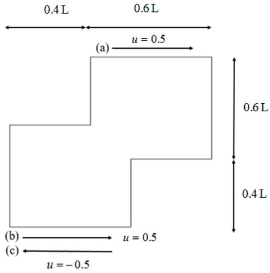
Figure 1.
Geometry of problem.
2. Mathematical Modeling
The physical illustration can be controlled through mathematical model. The subjects in which the mathematical model is used are computer science, political science, electrical engineering, chemistry, physics, biology, sociology, psychology and many more. The structuring mathematical model is known as mathematical modeling. The continuity equation and Navier-Stokes equations are generally acceptable differential equations for the field of Newtonian fluid rheology. To investigate flow field in staggered cavity the mathematics is reviewed as follows:
2.1. Continuity Equation
The general form of continuity equation is as follows:
the Equation (1) can be expressed alternatively as follows:
When the fluid flow is assumed to be two dimensional, steady and incompressible, than the Equation (2) reduces to
to obtain dimensionless form we have used
and hence the Equation (3) reduce to
2.2. Momentum Equation
The general vectorial notation of momentum equation can be written as:
In the absence of body force, for two dimensional, steady and an incompressible fluid flow, the component form of Equation (6) can be written as:
To achieve dimensionless system, we have used the following setup:
the governing Equations (7) and (8) reduce to
where, denotes Reynolds number.
2.3. Boundary Conditions
The left and right walls are manifested with no slip condition. The rest of boundary reading for each case is listing as follows:
| Case-I | (12) | |
| Upper wall velocity | ||
| Velocity of rest of walls | ||
| Case-II | (13) | |
| Upper wall velocity | ||
| Lower wall velocity | ||
| Velocity of rest of walls | ||
| Case-III | (14) | |
| Upper wall velocity | ||
| Lower wall velocity | ||
| Velocity of rest of walls | ||
3. Solution Procedure
It is important to note that one cannot find exact solution of Equations (10) and (11) along with boundary conditions provided in Equations (12)–(14), therefore, the finite element scheme is utilized to report the better approximation. A finite element method [39,40,41] is one of the most powerful numerical method and commonly used approach to solve the boundary value problems. This method has the application for the modeling and simulation of different physical phenomena in interconnect structures. For the finite element method the key six steps are
- Discretization of the domain.
- Establish simpler finite element equations.
- Assemble/Combine element equations.
- Incorporate the initial conditions or boundary constraints.
- Solve the developed equations.
- Post processing (Visualization).
To yield accuracy we discretize the computational domain with the help of both rectangular and triangular elements as hybrid meshing.
4. Analysis
The fluid flow narrating differential equations in a staggered enclosure are Equations (10) and (11) along with the boundary constraints provided in Equations (12)–(14) are solved numerically. For better novelty, the staggered cavity as a computational domain is discretized in nine different refinement levels. The lowest refinement level divide the cavity into 332 domain elements and 44 boundary elements.
The geometric illustration is offered in Figure 2. The level two in which the computational domain consists of 450 domain elements and 56 boundary elements is disclosed in Figure 3. The refinement level three is consists of 72 boundary elements and 724 domain elements is given in Figure 4. The four level consists of 108 boundary elements and 1272 domain elements and it is displayed in Figure 5. The Figure 6 shows that the level five consists of 1884 domain elements and 136 boundary elements. The six refinement level consists of 2950 domain elements and 172 boundary elements as illustrated in Figure 7. The level seven consists of 7248 domain elements and 340 boundary elements as shown in Figure 8. The Figure 9 depicts the level eight which consists of 18,664 domain elements and 652 boundary elements. Lastly, the highest level is the extremely fine which divides the cavity into 24,014 domain elements and 652 boundary elements is shown in Figure 10. The primitive variables namely, the velocity and pressure are evaluated at level-9 for all cases. The first case includes the motion of top wall with velocity and rest of walls are taken zero. The key to the graphs for this case are as follows: Figure 11 is velocity distribution at Re = 50. The velocity plot at Re = 100, Re = 400 and Re = 1000 are offered in Figure 12, Figure 13 and Figure 14 respectively. The pressure distribution at Re = 50, Re = 100, Re = 400 and Re = 1000 are provided in Figure 15, Figure 16, Figure 17 and Figure 18 respectively. For better insight the line graph study is executed to examine the u and v velocity profiles against variation in µ = 0.02 (Re = 25), µ = 0.01 (Re = 50), µ = 0.0025 (Re = 200), and µ = 0.001 (Re = 500). Such output is offered in Figure 19 and Figure 20. In detail, the velocity distribution in staggered cavity is examine at Re = 50 and the outcome is displayed in Figure 11. It is noticed that the streamlines near the top wall has maximum visibility and there are two secondary vortices appears in the left and right corners of the top wall. There is only one primary vortex appear at the center of upper region. Further, for Re = 100 there is a trifling change in the streamlines of the secondary vortices, see Figure 12. For Re = 400, the secondary vortex in right corner has prominent as compare to the secondary vortex in the left corner see Figure 13. The velocity distribution is examined at Re = 1000 and the one primary vortex is observed. The Figure 14 is plotted in this direction. One can note that the increase in Reynolds number cause prominence of secondary vortices. The corresponding pressure evaluation is recorded for Re = 50, Re = 100, Re = 400 and Re = 1000. In detail, Figure 15 is pressure distribution at Re = 50. It is noticed that the pressure seems maximum at corners of top wall. The Figure 16, Figure 17 and Figure 18 are pressure plots for Re = 100, Re = 400 and Re = 1000 respectively. It is noticed that the higher values of Reynolds number cause increase in pressure at top corners of staggered cavity.
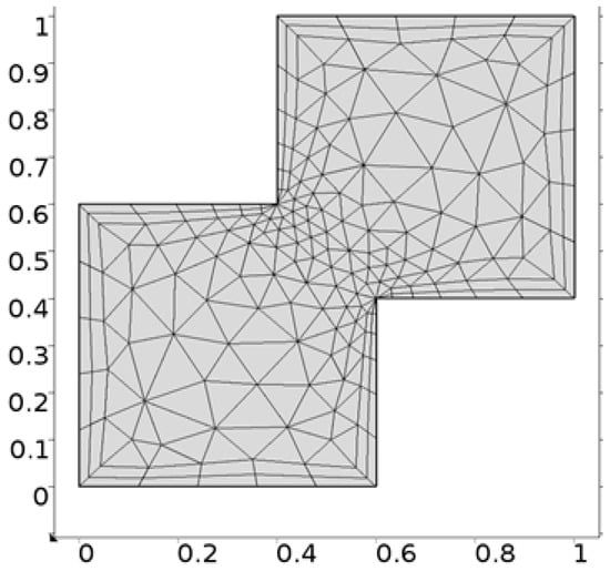
Figure 2.
Refinement level-1.
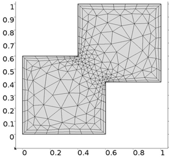
Figure 3.
Refinement level-2.

Figure 4.
Refinement level-3.
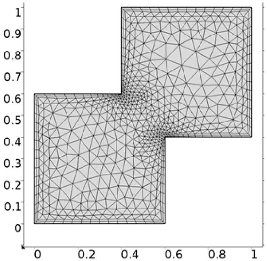
Figure 5.
Refinement level-4.

Figure 6.
Refinement level-5.
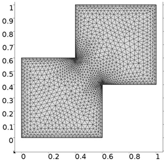
Figure 7.
Refinement level-6.

Figure 8.
Refinement level-7.
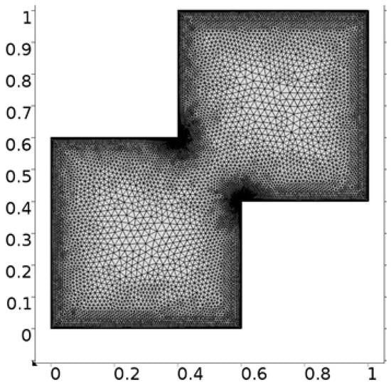
Figure 9.
Refinement level-8.
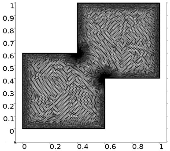
Figure 10.
Refinement level-9.
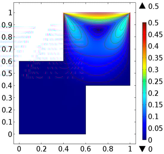
Figure 11.
Velocity distribution at Re = 50 for case-I.
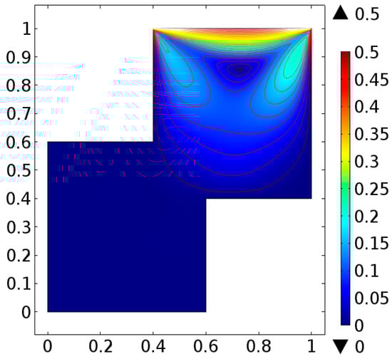
Figure 12.
Velocity distribution at Re = 100 for case-I.
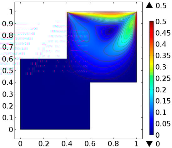
Figure 13.
Velocity distribution at Re = 400 for case-I.
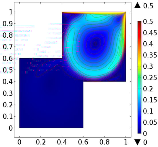
Figure 14.
Velocity distribution at Re = 1000 for case-I.
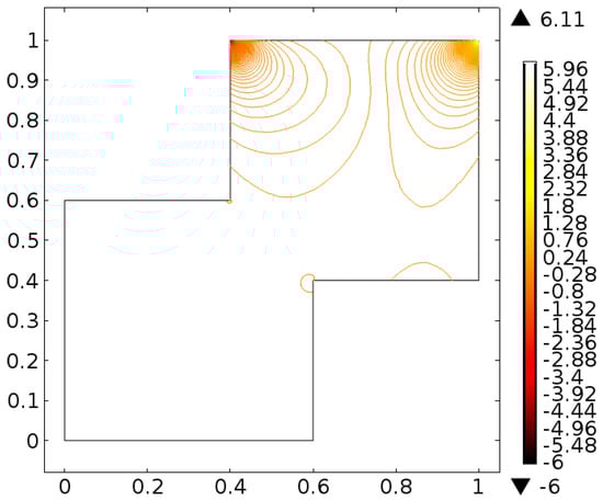
Figure 15.
Pressure distribution at Re = 50 for case-I.
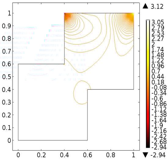
Figure 16.
Pressure distribution at Re = 100 for case-I.
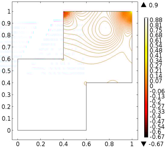
Figure 17.
Pressure distribution at Re = 400 for case-I.
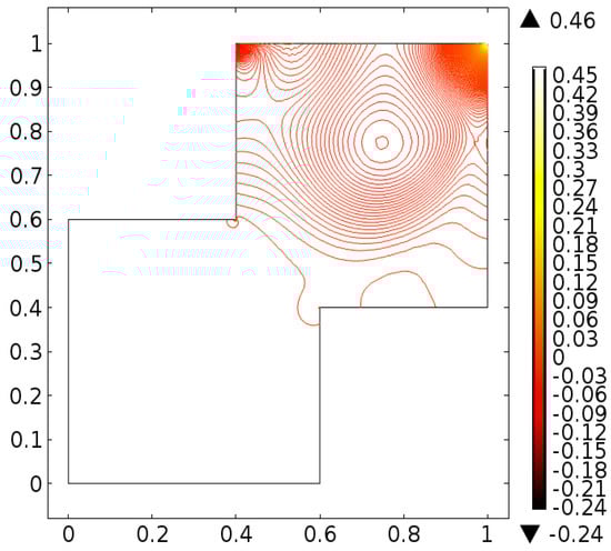
Figure 18.
Pressure distribution at Re = 1000 for case-I.
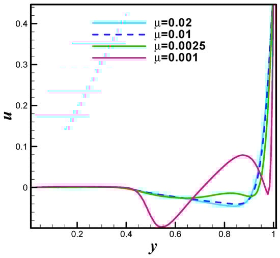
Figure 19.
The u-velocity profile for case-I.
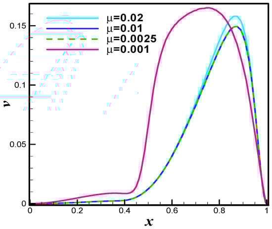
Figure 20.
The v-velocity profile for case-I.
The Figure 19 is u-velocity line graph at different values of µ = 0.02 (Re = 25), µ = 0.01 (Re = 50), µ = 0.0025 (Re = 200), and µ = 0.001 (Re = 500). The significant variation in the u-velocity is observed. Similar is the case for the v-velocity line graph see Figure 20. In case-II we assumed that the both top and bottom walls are moving in parallel with velocity and left and right walls are taken at rest. The velocity distribution is evaluated at level-9 for better accuracy. Figure 21 depicts the velocity distribution at Re = 50. Once can see that the uniform trends are observed in both upper and lower region of staggered cavity. The total of four secondary vortices in the left and right corners of the top and bottom wall and two primary vortices are appeared. The velocity distribution is inspected at Re = 100. The Figure 22 is evident in this direction. One can see that the secondary vortices becomes more visible. The velocity distribution at Re = 400 and Re = 1000 is examined and offered with the aid of Figure 23 and Figure 24 respectively. One can see that the increase in Reynolds cause significant deformation in primary and secondary vortices. The pressure distribution when upper and lower walls of staggered cavity are moving parallel is examined at various of Reynolds number. The adopted values of Reynolds number are Re = 50, Re = 100, Re = 400 and Re = 1000. To be more specific, the Figure 25 offers pressure plot at Re = 50. One can see that the pressure seems maximum at corns points of cavity. Figure 26, Figure 27 and Figure 28 are the pressure examination at Re = 100, Re = 400 and Re = 1000 respectively. It is observed that the higher values in Reynolds number results dense pressure at corns of staggered cavity. The Figure 29 is u-velocity line graph at different values of µ = 0.02 (Re = 25), µ = 0.01 (Re = 50), µ = 0.0025 (Re = 200), and µ = 0.001 (Re = 500). The significant variation in the u-velocity is observed while line graph study as v-velocity towards µ = 0.02 (Re = 25), µ = 0.01 (Re = 50), µ = 0.0025 (Re = 200), and µ = 0.001 (Re = 500) is offered in Figure 30. It is noticed that the v-velocity reflects inciting values towards higher values of Reynolds number. The case-III defines the antiparallel motion of the top and bottom wall with same velocity. The finite element simulation is performed by carrying hybrid meshing as a level-9. The primitive variables namely, the velocity and pressure are inspected towards higher values of Reynolds number. The adopted values of Reynolds number are Re = 50, Re = 100, Re = 400 and Re = 1000. In detail, the Figure 31 shows the velocity distribution at Re = 50 when the upper and lower walls are moving antiparallel. The primary and secondary vortices are formed in both upper and lower region of staggered cavity. The streamlines intersect at center region of cavity. The velocity distribution at Re = 100 is observed and offered in terms of graphical trend see Figure 32. One can see that the additional loop as a vortex is formed at the central region of staggered cavity.
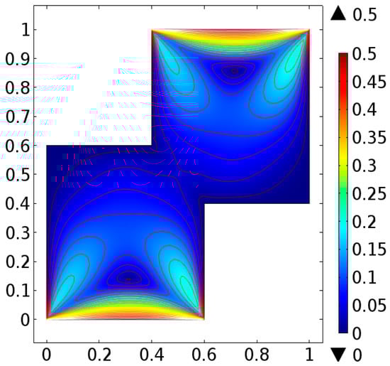
Figure 21.
Velocity distribution at Re = 50 for case-II.

Figure 22.
Velocity distribution at Re = 100 for case-II.
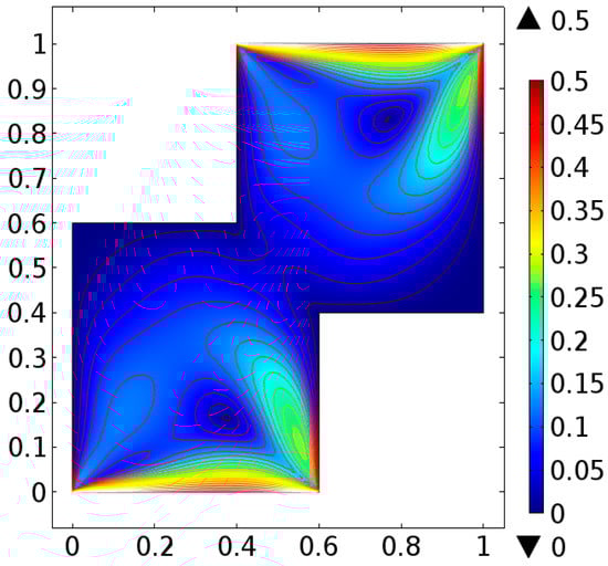
Figure 23.
Velocity distribution at Re = 400 for case-II.
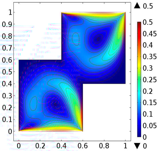
Figure 24.
Velocity distribution at Re = 1000 for case-II.
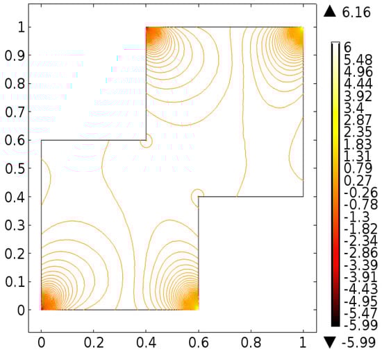
Figure 25.
Pressure distribution at Re = 50 for case-II.
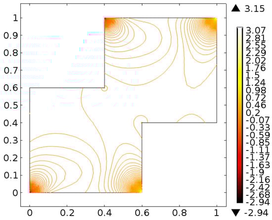
Figure 26.
Pressure distribution at Re = 100 for case-II.
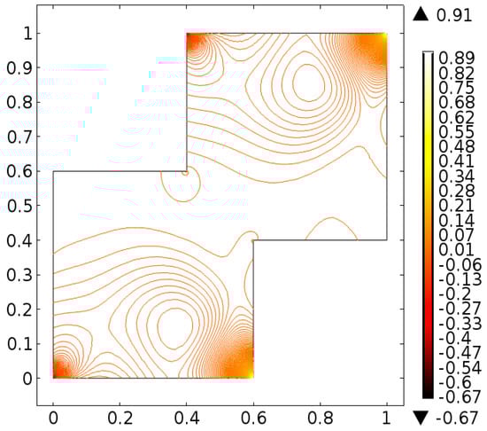
Figure 27.
Pressure distribution at Re = 400 for case-II.
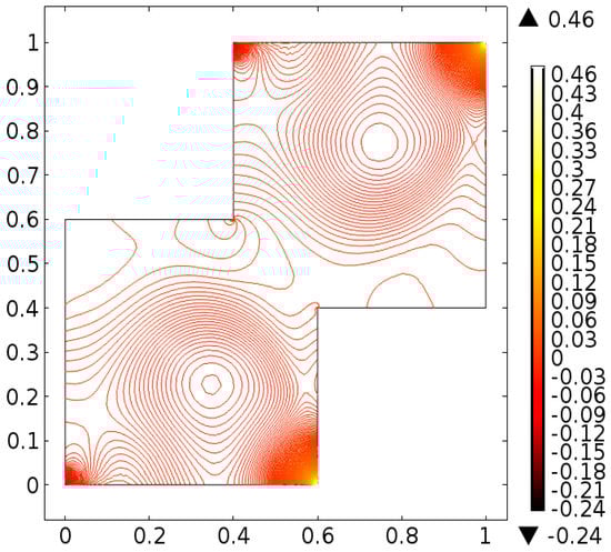
Figure 28.
Pressure distribution at Re = 1000 for case-II.
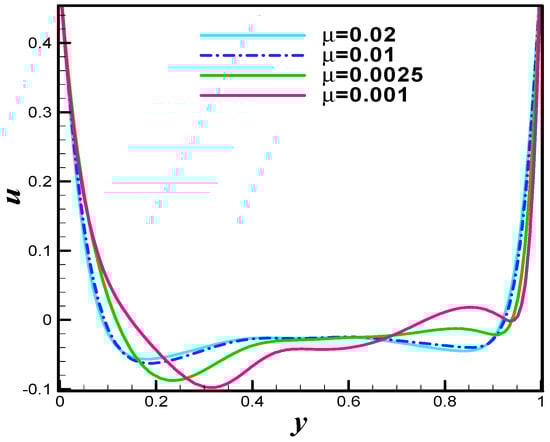
Figure 29.
The u-velocity profile for case-II.

Figure 30.
The v-velocity profile for case-I.
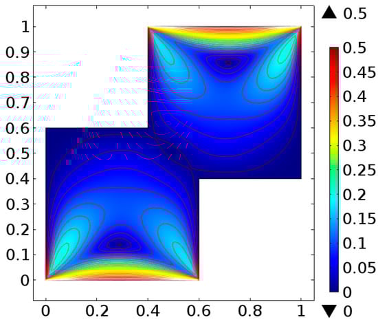
Figure 31.
Velocity distribution at Re = 50 for case-III.
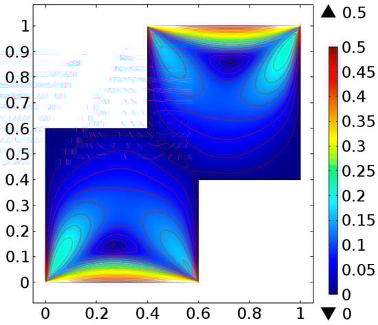
Figure 32.
Velocity distribution at Re = 100 for case-III.
The velocity distribution when top and bottom walls are moving antiparallel is observed at Re = 400 and Re = 1000. The Figure 33 and Figure 34 are plotted in this direction. It can be noticed from Figure 33 that the central region vortex shrinks by increasing Reynold number that is Re = 100. At Re = 1000, the primary vortices becomes dominant and vortex at central region of staggered shrinks significantly. The pressure plots when both walls namely upper and lower are moving antiparallel are offered at different values of Reynolds number that is Re = 50, Re = 100, Re = 400 and Re = 1000. Particularly, Figure 35 is pressure plot at Re = 50. Figure 36 is pressure plot at Re = 100 while the Figure 37 and Figure 38 are pressure distribution at Re = 400 and Re = 1000 respectively. Collectively, one can see that the pressure distribution becomes higher in strength against increasing values of Reynolds number. The line graph study of velocity distribution when walls are moving antiparallel is performed for both u and v components. In detail, the Figure 39 is u-velocity line graph at µ = 0.02 (Re = 25), µ = 0.01 (Re = 50), µ = 0.0025 (Re = 200), and µ = 0.001 (Re = 500) while Figure 40 offers the v-velocity line graph study towards µ = 0.02 (Re = 25), µ = 0.01 (Re = 50), µ = 0.0025 (Re = 200), and µ = 0.001 (Re = 500). The trifling sinusoid variation is observed for v-velocity. The kinetic energy is a very important benchmark quantity for the driven cavity flow problems which shows the momentum scale for the entire flow. It can be defined as
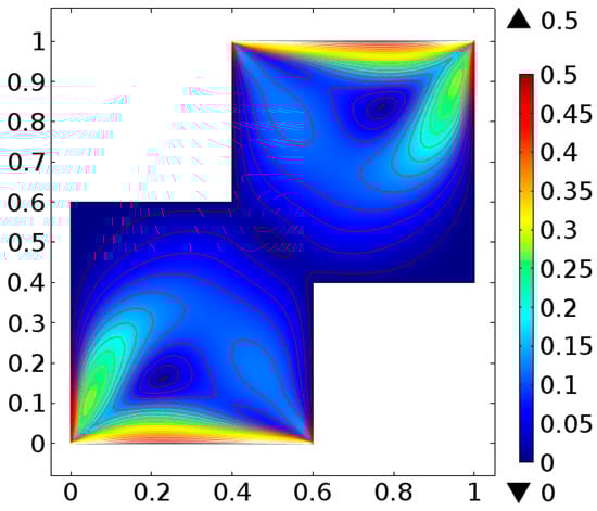
Figure 33.
Velocity distribution at Re = 400 for case-III.
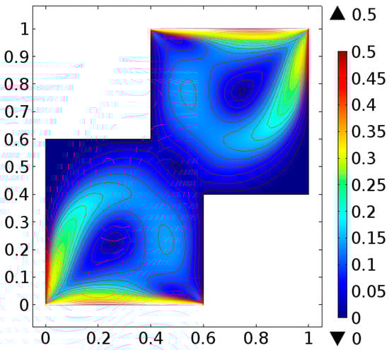
Figure 34.
Velocity distribution at Re = 1000 for case-III.
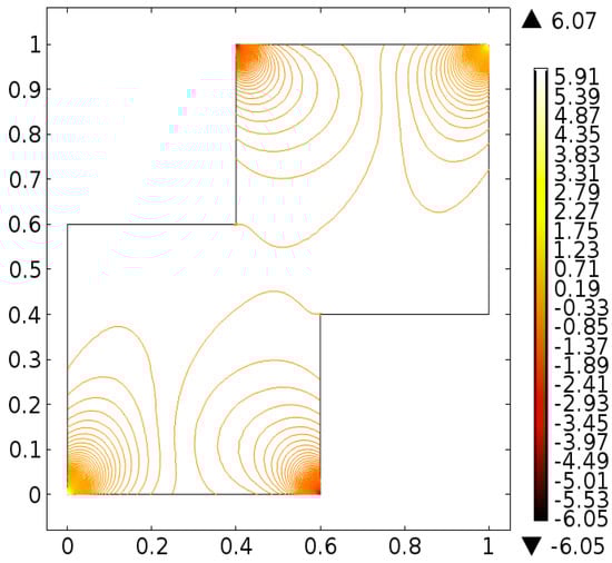
Figure 35.
Pressure distribution at Re = 50 for case-III.
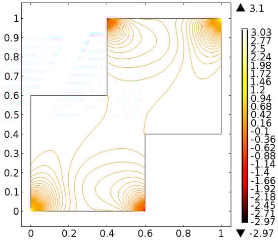
Figure 36.
Pressure distribution at Re = 100 for case-III.
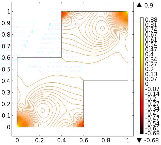
Figure 37.
Pressure distribution at Re = 400 for case-III.
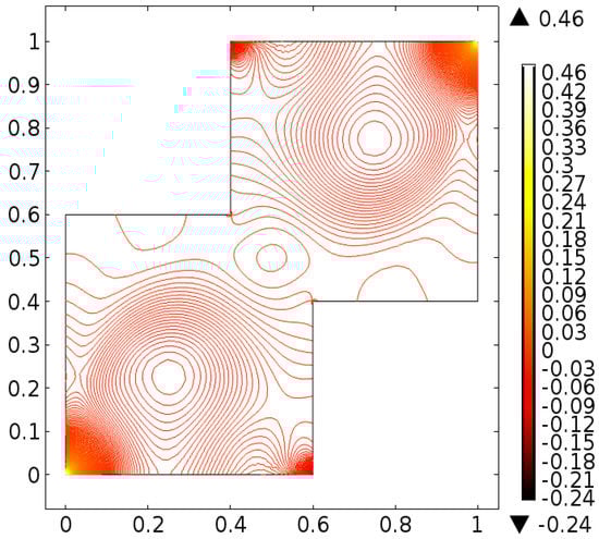
Figure 38.
Pressure distribution at Re = 1000 for case-III.
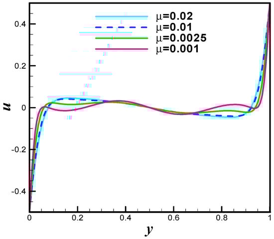
Figure 39.
The u-velocity profile for case-III.
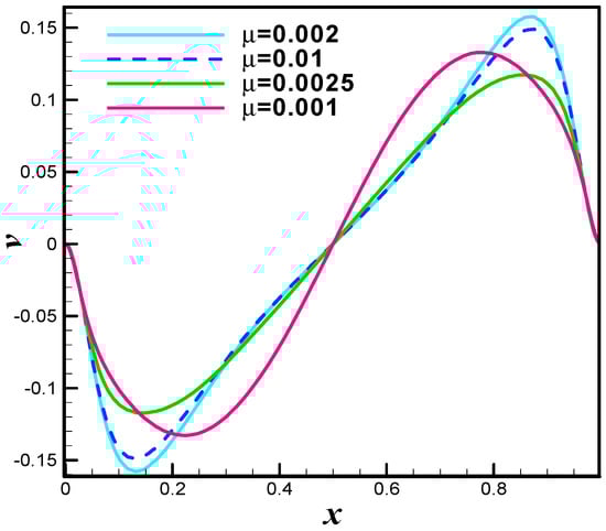
Figure 40.
The v-velocity profile for case-III.
To show the grid convergence, we tabulate the kinetic energy at different refinement levels at a fixed Re = 1000 shown in the Table 1. We can see that grid convergence is achieved for the kinetic energy at level 9. The variation in kinetic energy is recorded for case-I, case-II and case-III towards Reynolds number (by varying viscosity µ and fixing L = 1, U = 0.5). Table 2, Table 3 and Table 4 are plotted in this regard. In detail, Table 2 provides the value of kinetic energy when only the upper wall of staggered cavity is moving. The kinetic energy values when both the upper and lower walls are moving parallel are reported in Table 3. The values of kinetic energy in Table 4 are recorded when both upper and lower walls of staggered cavity are moving antiparallel.

Table 1.
Grid convergence for kinetic energy.
Table 2.
Kinetic energy values when only upper wall is moving.
Table 3.
Kinetic energy values when upper and lower walls are moving parallel.
Table 4.
Kinetic energy values when upper and lower walls are moving antiparallel.
5. Conclusions
The fluid equipped in staggered cavity is examined. The Newtonian fluid model is entertained. The detail analysis is performed for three different cases. The first includes the motion of upper wall of staggered cavity with uniform velocity. In second case both upper and lower walls are moving in parallel direction and in third case the walls namely upper and lower are moving in an antiparallel direction. The solution is obtained by finite element method and formulation of both the primary vortices, secondary vortices and kinetic energy variation are debated for each case. We trusted that this attempt will provide a directory for the investigators to handle unsolved problems in the field of enclosure having uses in an industry and engineering areas.
Author Contributions
K.U.R. and N.K. conceived and designed the experiments; N.F. performed the experiments; W.A.K. and N.K. analyzed the data; W.A.K. contributed reagents/materials/analysis tools; K.U.R. wrote the paper. All authors have read and agreed to the published version of the manuscript.
Funding
The authors received no financial support for the research, authorship and/or publication of this article.
Acknowledgments
The authors are very thankful for the anonymous referees whose suggestions and comments helped to improve the quality of the manuscript.
Conflicts of Interest
The authors declare no conflict of interest.
Nomenclature
| Dimensional space variables | |
| Dimensionless space variables | |
| Dimensional velocity field | |
| Dimensionless velocity field | |
| Fluid density | |
| Characteristic length | |
| Reference velocity | |
| Dimensional pressure | |
| Dimensionless pressure | |
| Reynolds number | |
| Dynamic viscosity | |
| Body force | |
| Del operator |
References
- Crane, L.J. Flow past a stretching plate. Z. Angew. Math. Phys. ZAMP 1970, 21, 645–647. [Google Scholar] [CrossRef]
- Devi, C.; Takhar, H.; Nath, G. Unsteady, three-dimensional, boundary-layer flow due to a stretching surface. Int. J. Heat Mass Transf. 1986, 29, 1996–1999. [Google Scholar] [CrossRef]
- Smith, S.H. An Exact Solution of the Unsteady Navier-Stokes Equations Resulting from a Stretching Surface. J. Appl. Mech. 1994, 61, 629–633. [Google Scholar] [CrossRef]
- Pop, I.; Na, T.-Y. Unsteady flow past a stretching sheet. Mech. Res. Commun. 1996, 23, 413–422. [Google Scholar] [CrossRef]
- Chiam, T. Heat transfer with variable conductivity in a stagnation-point flow towards a stretching sheet. Int. Commun. Heat Mass Transf. 1996, 23, 239–248. [Google Scholar] [CrossRef]
- Vajravelu, K.; Hadjinicolaou, A. Convective heat transfer in an electrically conducting fluid at a stretching surface with uniform free stream. Int. J. Eng. Sci. 1997, 35, 1237–1244. [Google Scholar] [CrossRef]
- Chamkha, A.J. Unsteady hydromagnetic flow and heat transfer from a non-isothermal stretching sheet immersed in a porous medium. Int. Commun. Heat Mass Transf. 1998, 25, 899–906. [Google Scholar] [CrossRef]
- Sarma, M.; Rao, B. Heat Transfer in a Viscoelastic Fluid over a Stretching Sheet. J. Math. Anal. Appl. 1998, 222, 268–275. [Google Scholar] [CrossRef]
- Subhas, A.; Veena, P. Visco-elastic fluid flow and heat transfer in a porous medium over a stretching sheet. Int. J. Non-linear Mech. 1998, 33, 531–540. [Google Scholar] [CrossRef]
- Vajravelu, K.; Roper, T. Flow and heat transfer in a second grade fluid over a stretching sheet. Int. J. Non-Linear Mech. 1999, 34, 1031–1036. [Google Scholar] [CrossRef]
- Yürüsoy, M.; Pakdemirli, M. Exact solutions of boundary layer equations of a special non-Newtonian fluid over a stretching sheet. Mech. Res. Commun. 1999, 26, 171–175. [Google Scholar] [CrossRef]
- Takhar, H.; Chamkha, A.; Nath, G. Flow and mass transfer on a stretching sheet with a magnetic field and chemically reactive species. Int. J. Eng. Sci. 2000, 38, 1303–1314. [Google Scholar] [CrossRef]
- Andersson, H.I.; Aarseth, J.B.; Dandapat, B.S. Heat transfer in a liquid film on an unsteady stretching surface. Int. J. Heat Mass Transf. 2000, 43, 69–74. [Google Scholar] [CrossRef]
- Vajravelu, K. Viscous flow over a nonlinearly stretching sheet. Appl. Math. Comput. 2001, 124, 281–288. [Google Scholar] [CrossRef]
- Abel, M.; Khan, S.K.; Prasad, K. Study of visco-elastic fluid flow and heat transfer over a stretching sheet with variable viscosity. Int. J. Non-Linear Mech. 2002, 37, 81–88. [Google Scholar] [CrossRef]
- Prasad, K.; Abel, S.; Datti, P. Diffusion of chemically reactive species of a non-Newtonian fluid immersed in a porous medium over a stretching sheet. Int. J. Non-Linear Mech. 2003, 38, 651–657. [Google Scholar] [CrossRef]
- Nazar, R.; Amin, N.; Filip, D.; Pop, I. Stagnation point flow of a micropolar fluid towards a stretching sheet. Int. J. Non-Linear Mech. 2004, 39, 1227–1235. [Google Scholar] [CrossRef]
- Mukhopadhyay, S.; Layek, G.; Samad, S. Study of MHD boundary layer flow over a heated stretching sheet with variable viscosity. Int. J. Heat Mass Transf. 2005, 48, 4460–4466. [Google Scholar] [CrossRef]
- Hsiao, K.-L. Conjugate heat transfer of magnetic mixed convection with radiative and viscous dissipation effects for second-grade viscoelastic fluid past a stretching sheet. Appl. Therm. Eng. 2007, 27, 1895–1903. [Google Scholar] [CrossRef]
- Abel, M.S.; Nandeppanavar, M.M. Heat transfer in MHD viscoelastic boundary layer flow over a stretching sheet with non-uniform heat source/sink. Commun. Nonlinear Sci. Numer. Simul. 2009, 14, 2120–2131. [Google Scholar] [CrossRef]
- Kelson, N.A. Note on similarity solutions for viscous flow over an impermeable and non-linearly (quadratic) stretching sheet. Int. J. Non-Linear Mech. 2011, 46, 1090–1091. [Google Scholar] [CrossRef]
- Ganga, B.; Saranya, S.; Ganesh, N.V.; Hakeem, A.K.A.; Vishnu, G.N.; Abdul, H.A. Effects of space and temperature dependent internal heat generation/absorption on MHD flow of a nanofluid over a stretching sheet. J. Hydrodyn. 2015, 27, 945–954. [Google Scholar] [CrossRef]
- Bilal, S.; Rehman, K.U.; Jamil, H.; Malik, M.Y.; Salahuddin, T. Dissipative slip flow along heat and mass transfer over a vertically rotating cone by way of chemical reaction with Dufour and Soret effects. AIP Adv. 2016, 6, 125125. [Google Scholar] [CrossRef]
- Seth, G.S.; Mishra, M. Analysis of transient flow of MHD nanofluid past a non-linear stretching sheet considering Navier’s slip boundary condition. Adv. Powder Technol. 2017, 28, 375–384. [Google Scholar] [CrossRef]
- Rehman, K.U.; Khan, A.A.; Malik, M.; Ali, U. Mutual effects of stratification and mixed convection on Williamson fluid flow under stagnation region towards an inclined cylindrical surface. MethodsX 2017, 4, 429–444. [Google Scholar] [CrossRef]
- Awais, M.; Rehman, K.-U.; Malik, M.Y.; Hussain, A.; Salahuddin, T. A computational analysis subject to thermophysical aspects of Sisko fluid flow over a cylindrical surface. Eur. Phys. J. Plus 2017, 132, 392. [Google Scholar] [CrossRef]
- Rehman, K.U.; Malik, A.A.; Malik, M.; Hayat, T. Generalized Lie symmetry analysis for non-linear differential equations: A purely viscous fluid model. Results Phys. 2017, 7, 3537–3542. [Google Scholar] [CrossRef]
- Bibi, M.; Rehman, K.-U.; Malik, M.Y.; Tahir, M. Numerical study of unsteady Williamson fluid flow and heat transfer in the presence of MHD through a permeable stretching surface. Eur. Phys. J. Plus. 2018, 133, 154. [Google Scholar] [CrossRef]
- Rehman, K.U.; Alshomrani, A.S.; Malik, M.; Zehra, I.; Naseer, M. Thermo-physical aspects in tangent hyperbolic fluid flow regime: A short communication. Case Stud. Therm. Eng. 2018, 12, 203–212. [Google Scholar] [CrossRef]
- Rehman, K.U.; Shahzadi, I.; Malik, M.; Al-Mdallal, Q.M.; Zahri, M. On heat transfer in the presence of nano-sized particles suspended in a magnetized rotatory flow field. Case Stud. Therm. Eng. 2019, 14, 100457. [Google Scholar] [CrossRef]
- Jalili, B.; Sadighi, S.; Jalili, P.; Ganji, D.D. Characteristics of ferrofluid flow over a stretching sheet with suction and injection. Case Stud. Therm. Eng. 2019, 14, 100470. [Google Scholar] [CrossRef]
- Ali, U.; Rehman, K.U.; Malik, M.Y. The influence of MHD and heat generation/absorption in a Newtonian flow field manifested with a Cattaneo-Christov heat flux model. Phys. Scr. 2019, 94, 085217. [Google Scholar] [CrossRef]
- Patil, D.; Lakshmisha, K.; Rogg, B.; Patil, D. Lattice Boltzmann simulation of lid-driven flow in deep cavities. Comput. Fluids 2006, 35, 1116–1125. [Google Scholar] [CrossRef]
- Dos Santos, D.D.; Frey, S.; Naccache, M.F.; Mendes, P.D.S.; Mendes, P.D.S. Numerical approximations for flow of viscoplastic fluids in a lid-driven cavity. J. Non-Newton. Fluid Mech. 2011, 166, 667–679. [Google Scholar] [CrossRef]
- ElShehabey, H.M.; Ahmed, S.E. MHD mixed convection in a lid-driven cavity filled by a nanofluid with sinusoidal temperature distribution on the both vertical walls using Buongiorno’s nanofluid model. Int. J. Heat Mass Transf. 2015, 88, 181–202. [Google Scholar] [CrossRef]
- Gutt, R.; Grosan, T. On the lid-driven problem in a porous cavity. A theoretical and numerical approach. Appl. Math. Comput. 2015, 266, 1070–1082. [Google Scholar] [CrossRef]
- Ding, P. Solution of lid-driven cavity problems with an improved SIMPLE algorithm at high Reynolds numbers. Int. J. Heat Mass Transf. 2017, 115, 942–954. [Google Scholar] [CrossRef]
- Indukuri, J.V.; Maniyeri, R. Numerical simulation of oscillating lid driven square cavity. Alex. Eng. J. 2018, 57, 2609–2625. [Google Scholar] [CrossRef]
- Templeton, J.A.; Jones, R.E.; Lee, J.W.; Zimmerman, J.A.; Wong, B.M. A Long-Range Electric Field Solver for Molecular Dynamics Based on Atomistic-to-Continuum Modeling. J. Chem. Theory Comput. 2011, 7, 1736–1749. [Google Scholar] [CrossRef]
- Mahmood, R.; Kousar, N.; Rehman, K.U.; Mohasan, M. Lid driven flow field statistics: A non-conforming finite element Simulation. Phys. A Stat. Mech. Appl. 2019, 528, 121198. [Google Scholar] [CrossRef]
- Liu, X.; Liu, L. An immersed transitional interface finite element method for fluid interacting with rigid/deformable solid. Eng. Appl. Comput. Fluid Mech. 2019, 13, 337–358. [Google Scholar] [CrossRef]


© 2020 by the authors. Licensee MDPI, Basel, Switzerland. This article is an open access article distributed under the terms and conditions of the Creative Commons Attribution (CC BY) license (http://creativecommons.org/licenses/by/4.0/).