Evaluation of the Turbulence Model Influence on the Numerical Simulation of Cavitating Flow with Emphasis on Temperature Effect


1
Institute for Energy Research, Jiangsu University, 301 Xuefu Road, Zhenjiang 212013, China
2
Research Center of Fluid Machinery Engineering and Technology, Jiangsu University, 301 Xuefu Road, Zhenjiang 212013, China
*
Author to whom correspondence should be addressed.
Processes 2020, 8(8), 997; https://doi.org/10.3390/pr8080997
Submission received: 20 July 2020
/
Revised: 9 August 2020
/
Accepted: 13 August 2020
/
Published: 17 August 2020
(This article belongs to the Section Chemical Processes and Systems)
Abstract
:The aim of this paper is to investigate the influence of different turbulence models (, RNG , and SST ) on the numerical simulation of cavitating flow in thermosensitive fluid. The filter-based model and density correction method were employed to correct the turbulent viscosity of the three turbulence models. Numerical results obtained were compared to experimental ones which were conducted on the NACA0015 hydrofoil at different temperatures. The applicability of the numerical solutions of different turbulence model was studied in detail. The modified RNG model has higher accuracy in the calculation of cavitating flow at different temperatures.
1. Introduction
Cavitation is an important issue that affects the operation and working life of fluid machinery. Cavitation refers to the process of the formation, development, and collapse of vapor cavities in the liquid or at the liquid–solid interface when the local pressure in the liquid decreases [1]. The pressure reduction and unsteady characteristics of the cavitation area usually lead to mechanical vibration and noise, resulting in negative effects such as equipment surface fatigue damage, fracture, and mechanical performance degradation [2,3,4].
When cavitation occurs, the fluid medium will absorb heat from the surrounding fluid due to the latent heat of vaporization during the transition from the liquid phase to the vapor phase, resulting in a decrease in the temperature of the cavitation zone—that is, the thermal effect on cavitation [5]. At normal temperature, the cavitation of water can ignore the influence of thermodynamic effects—that is, when the cavitation occurs, it is assumed that the temperature of the cavitation area does not change [6,7]. However, the physical properties of thermosensitive fluid such as liquid hydrogen, liquid nitrogen, and liquid oxygen are sensitive to temperature changes. During the cavitating flow, the thermodynamic effect is significant, which causes the temperature of the cavitation region to change, which changes the cavitating flow field dramatically [8,9,10].
Fluids such as liquid hydrogen and liquid oxygen are often used as propellants for liquid carrier rocket engines. Because the weight and size of the engine turbo pump are subject to strict design requirements, it is necessary to increase the engine thrust by increasing the power density of the turbo pump. At the same time, in order to ensure effective carrying capacity, reducing the volume of the propellant container will cause the pressure at the entrance of the inducer to decrease. Under the conditions of high-speed rotation and lower inlet pressure, cavitation can easily occur around the blade of the inducer, making its internal flow field unstable and causing strong mechanical vibration, thereby reducing the reliability and stability of the rocket engine. Therefore, in-depth research on the cavitating flow characteristics of thermosensitive fluids has important theoretical value and engineering application significance [11,12].
Under the thermodynamic effect, cavitating flow is a complex fluid dynamics problem involving phase transition, turbulence, heat transfer, and other phenomena. In the early stage, the process of cavitation flow under thermodynamic effects was mainly observed and analyzed by experimental research. Hord [13,14] conducted experimental research about the cavitating flow around hydrofoils and ogives. The liquid hydrogen and liquid nitrogen were employed as the working fluid. The cavity length and the pressure and temperature distributions were obtained under different working conditions. The experimental results have been widely used as a verification standard to evaluate the correctness of different cavitation models. Due to the difficulty of conducting experimental research in related aspects and the limited measurement of flow field data in the cavitation area, numerical simulation technology has gradually become an important alternative to study the cavitating flow behavior.
From the perspective of computational fluid dynamics (CFD), turbulence model and cavitation model play significant roles in the numerical simulation of cavitating flow in thermosensitive fluids. For the cavitation model, a modified Merkle cavitation model has been demonstrated to be effective in simulating cryogenic fluids [15]. For the turbulence model, the prediction and solution of turbulent flow in numerical calculation are mainly divided into three categories: direct numerical simulation (DNS), large eddy simulation (LES), and Reynolds-averaged Navier–Stokes simulation (RANS).
The DNS method [16,17] obtains turbulent flow in all time and space scales in the flow field by directly solving the Navier–Stokes equation. Although this method is the most accurate method for simulating turbulent flow in the flow field, it has extremely high requirements on computer performance. It is also still difficult to solve complex engineering problems. The LES method [18,19] uses low-pass filtering on the Navier–Stokes equation to reduce the solution on the space and time scales, thereby directly solving large-scale vortices in turbulent flow, and making model assumptions on the motion of small-scale vortices. The calculation accuracy of the LES method is high [20,21]. Although a large amount of calculation resources is still required, it is also increasingly used in actual engineering calculations. The RANS method [22,23] uses the time average method to decompose the flow into time average flow and instantaneous pulsating flow, and solves them separately. This method avoids directly solving the Navier–Stokes equation, saving a lot of computing resources while ensuring the calculation accuracy, and has achieved good results in practical applications. Therefore, this article uses the RANS method to solve the problem of cavitation flow under thermodynamic effect. However, the overestimate of the eddy viscosity restricts the use of the RANS method in accurate simulation of cavitating flow. For the above reason, many researchers focused on the correction of eddy viscosity such as the density-corrected model (DCM) [24,25] and filter-based model (FBM) [26,27]. Due to the significant change in density ratio, the DCM primarily amends the viscosity corresponding to the highly compressible area, while FBM pays attention to enhance the resolution to capture finer flow characteristics.
The purpose of this paper is to excavate an effective turbulence model for simulating cavitating flow considering thermosensitive fluids. Various turbulence models, including the standard model, RNG (re-normalization group) model, and SST (shear-stress transport) model, were modified by the density-corrected model and filter-based model. The numerical simulations were performed around a three-dimensional NACA (National Advisory Committee for Aeronautics) 0015 hydrofoil with the commercial CFD code ANSYS CFX. The pressure coefficients at different temperatures were investigated numerically and experimentally. The simulation results are used to assess the applicability and feasibility of different turbulence models for the simulation of cavitating flow in cryogenic fluids.
2. Mathematical Formation
2.1. Governing Equations
The thermosensitive cavitating flow is treated as the homogeneous multiphase flow. The continuity, momentum, and energy equations in the Cartesian coordinates are shown as follows:
where is the density of multiphase flow, subscripts v and l mean vapor phase and liquid phase, respectively; subscripts i and j represent the coordinates in the Cartesian coordinate system; is the volume fraction; u is the flow velocity; p is the pressure in the flow field; μm is the dynamic viscosity; μt is the turbulent dynamic viscosity; is the effective thermal conductivity; T is temperature; is specific heat; and L is the latent heat.
2.2. Turbulence Model
For the turbulence model, how to predict the turbulent eddy viscosity in the cavitation area is a key problem, affecting the accuracy of numerical simulation results. In this study, DCM and FBM are employed to modify the turbulent eddy viscosity for three turbulence models (, RNG , and SST ). The implementation in detail is shown below.
2.2.1. Turbulence Model
This model is a classic two-equation turbulence model with good applicability and high utilization frequency. It has been embedded in many CFD solvers. The specific form of the equation is as follows:
For the turbulent kinetic energy equation,
For the turbulent dissipation rate equation,
For the turbulent viscosity,
In the formula, , , , , and are all empirical coefficients, taking the values of 1.44, 1.92, 1.0, 1.3, and 0.09, respectively. Pkb and Pεb are the influence source terms of buoyancy, and Pk is the turbulent kinetic energy generation term.
2.2.2. RNG Turbulence Model
When there is a strong vortex motion and a large fluid pressure gradient in the flow field, the prediction accuracy of k-ε turbulence model is limited. Compared with the k-ε turbulence model, the RNG k-ε model considers the rotating flow. The time-averaged strain rate is also considered in the turbulent energy dissipation rate equation.
For the turbulent kinetic energy equation,
For the turbulent dissipation rate equation,
In the formula, the value of each constant is: Cε2RNG = 1.68, βRNG = 0.012, CμRNG = 0.085.
2.2.3. SST Turbulence Model
The standard k-ε model and its improved RNG k-ε model have higher simulation accuracy for the turbulent flow that has been fully developed on the far wall surface, but the accuracy of flow simulation with flow separation phenomena and large backpressure gradients needs to be improved. Menter [28] proposes a two-equation SST k-ω model, which is obtained by modifying the (baseline) BSL k-ω model. The simulation accuracy of separated flow and strong curvature flow is greatly improved, but there are problems such as high requirements on grid resolution, difficulty in convergence, and sensitivity to boundary conditions. The equation expression is as follows:
For the turbulent kinetic energy equation,
For the turbulence frequency equation,
For the turbulent viscosity equation,
where is the turbulent kinetic energy term produced by buoyance; is the turbulent kinetic energy term produced by viscous force; F1 and F2 are the blending functions; and S is the shear tensor. The constant coefficients are taken separately: a1 = 0.31, σk = 2, β’ = 0.09, σω = 2, α = 5/9, β = 0.075, and σω2 = 1/0.856.
The expressions of F1 and F2 are as follows:
where V is kinematic viscosity.
2.2.4. Modification of Turbulence Model
Considering the influence of turbulence scale and the compressibility of gas–liquid mixed phase, the filter-based model and density correction method are employed to modify the turbulent viscosity of three turbulence models, which was used for the following numerical study:
where C3 is the empirical coefficients, which is assigned to be 1.0.
2.3. Cavitation Model for Thermosensitive Fluids
With the evolution of the cavitation process, the mass transfer rate between liquid phase and vapor phase is controlled by the combination of source term m+ and sink term m−, respectively. To capture the cavitation characteristics, liquid volume fraction and vapor volume fraction needs to be obtained. A representative method is to employ a transport equation to determine the liquid volume fraction and vapor volume fraction, respectively. For the Merkle cavitation model [29], the transfer rate between the liquid phase and vapor phase is supposed to be proportional to the local pressure difference. The governing equation for the Merkle cavitation model is shown below:
where and are the characteristic constant coefficients for the evaporation and condensation, respectively; is the reference speed at infinity; is the reference time; and pv is the saturated vapor pressure. The default values for and are listed as follows:
The original Merkle cavitation model [29] is established based on the isothermal assumption. The saturated vapor pressure in the model is a fixed value, while the saturated vapor pressure of thermosensitive fluid is actually a function of temperature. In our previous study, the B-factor theory and Antoine equation were taken into consideration. Considering the influence of turbulent kinetic energy on the saturated vapor pressure, the modified source term is shown as follows:
For the implementation of the corrected turbulence model and cavitation model in the numerical simulation, the CEL language assembly function is employed to embed them in CCL files into the CFX software.
3. Numerical Setup and Validation
The numerical results were validated by a recognized cavitation experiment conducted by Cervone et al. [30]. Water at different temperatures around the NACA0015 hydrofoil were investigated experimentally in the Cavitating Pump Rotordynamic Test Facility (CPRTF) laboratory. The influence of thermodynamic effect on the cavitation performance was analyzed. The experimental data was published in the American Society of Mechanical Engineers (ASME) journal, which attracted great attention from the research community.
3.1. NACA0015 Hydrofoil Geometry Model
The structure of NACA0015 hydrofoil used in the experiment is shown in Figure 1. The hydrofoil chord has a length of 115 mm and a width of 80 mm. The attack angle of the experimental hydrofoil ranges from 4° to 8°. There are three holes for pressure measurement at the inlet and outlet of the experimental section, ten holes for pressure measurement along the suction surface of the hydrofoil, and two holes for pressure measurement along the pressure surface of the hydrofoil. The model is built using the UG software. The 3D model of NACA0015 hydrofoil is shown in Figure 2.
3.2. Mesh Implementation
The ICEM CFD software is employed to mesh the NACA0015 hydrofoil into a hexahedral structured grid. The mesh grid around the NACA0015 hydrofoil is shown in Figure 3. The mesh quality of the boundary layer around the hydrofoil has a great influence on the accuracy of numerical simulation results. The y+ value is usually employed to judge the mesh quality [31,32]. There is no specific range for the distribution of the y+ value for different turbulence models. The y+ value is usually maintained under 60 to keep the accuracy of the simulation results in the research community. In order to improve the quality of the mesh grid, a refined C-shaped structure grid is used around the leading edge and trailing edge of the hydrofoil. The distribution of the y+ value on the upper and lower surfaces of the hydrofoil is shown in Figure 4.
3.3. Boundary Conditions
The boundary conditions for the numerical setup is shown in Figure 2. The inlet is set to be the velocity inlet boundary condition, the outlet is set to be the pressure outlet boundary condition, and the wall is set to be the non-slip boundary condition. The specific values at different temperatures are listed in Table 1.
3.4. Mesh Independence Study
Three sets of meshes with different densification levels, namely mesh 1, mesh 2, and mesh 3, are employed to perform the mesh independence study. The mesh information is shown in Table 2. To facilitate comparison and verification, the dimensionless pressure coefficient is defined as follows:
where is pressure at outlet; is speed at inlet; and is the density of the working fluid.
The number of grids in the three sets (mesh 1, mesh 2 and mesh 3) are 1.1 million, 2.85 million, and 4.56 million, respectively. As shown in Figure 5, the simulated pressure coefficients along the upper surface of NACA0015 hydrofoil match well with the experimental results. Taking the calculation cost into consideration, mesh 2 is selected in the numerical simulation.
4. Results and Discussion
4.1. Influence of Different Turbulence Models on NACA0015 at 25 °C
Using three turbulence models and their corresponding modified turbulence models, the numerical simulation about the cavitating flow around the NACA0015 hydrofoil is performed. The distribution of pressure coefficient along the suction side of the NACA0015 hydrofoil is obtained as shown in Figure 6. The results show that there is a certain difference between the simulated pressure coefficient and experimentally measured pressure coefficient in the low-pressure area of the first 30% of the hydrofoil length. At the last 70% of the hydrofoil length, the calculation results of the RNG k-ε and SST k-ω turbulence models are closer to the experimental values, and the simulation results of the k-ε model differ greatly from the experimental results. Based on the modified turbulence model, the simulation results of the revised RNG k-ε model and the revised SST k-ω showed significant improvement, which is closer to the experimental value. The simulation results of the revised k-ε model are significantly smaller than that of the uncorrected turbulence model. The correction effect is obvious.
The root-mean-square (RMS) error and maximum deviation of the pressure coefficient for the numerical and the experimental results were analyzed to demonstrate the improvement of the calculation results of the three turbulence models and their modified turbulence models. The RMS error and the maximum deviation are shown in Figure 7. The results showed that the RMS error and the maximum deviation of the RNG k-ε model and the SST k-ω model are less than that of the k-ε model; meanwhile, the RMS error and the maximum deviation of the modified turbulence model showed good improvement.
At room temperature, the distribution of vapor volume fractions on the surface of NACA0015 hydrofoil is shown in Figure 8. The results showed that the k-ε model has a large-scale vortex at the tail of the cavity, and the development process of the cavitation core area is longer. Meanwhile, the development process of RNG k-ε model and SST k-ω model in the cavitation core area is shorter. The modified k-ε model eliminates the vortex at the tail of the cavity, but the cavitation core area is significantly shorter. The cavitation area is significantly expanded based on the modified RNG k-ε model and the modified SST k-ω model and the vapor volume fraction in the cavitation core area is larger.
4.2. Influence of Different Turbulence Models on NACA0015 at 50 °C
Through the discussion in Section 4.1, the modified RNG k-ε model and the modified SST k-ω model show good applicability. This section focuses on the modified RNG k-ε model and the SST k-ω model for the numerical simulation of cavitating flow around the NACA0015 hydrofoil at 50 °C and compares it with the experimental results.
At 50 °C, the pressure coefficient distribution of the NACA0015 hydrofoil suction surface simulated by the modified RNG k-ε model and the modified SST k-ω model is shown in Figure 9. The revised RNG k-ε model calculates the low-pressure region in a small range, while the revised SST k-ω model calculates the low-pressure region in a large range. The RMS error and the maximum deviation are shown in Figure 10. The results show that at 50 °C, the RMS error and maximum deviation of the modified SST k-ω model are both less than that of the modified RNG k-ε model.
4.3. Influence of Different Turbulence Models on NACA0015 at 70 °C
Figure 11 shows the distribution of the pressure coefficient along the suction surface of the NACA0015 hydrofoil simulated by the modified RNG k-ε model and the modified SST k-ω model at 70 °C. The results show that the simulation using revised RNG k-ε model matches well with the experimental results. The modified SST k-ω model has a longer cavitation development process. Figure 12 shows that the RMS error and maximum deviation of the modified RNG k-ε model are less than that of the modified SST k-ω model. The corrected RNG k-ε model is more accurate at 70 °C.
4.4. Influence of Modified RNG k-ε Model on NACA0015 Hydrofoil at Different Temperatures
Figure 13 shows the vapor volume fraction distribution on the surface of NACA0015 hydrofoil calculated by the modified RNG k-ε model at different water temperatures. The results show that as the temperature increases, the vapor volume fraction decreases, the cavity area decreases, and the vapor–liquid interface becomes blurred. The water vapor content decreases with the increase of temperature.
5. Conclusions
This paper carries out numerical investigation of different turbulence model effect on the cavitating flow around NACA0015 hydrofoil with water at different temperatures. The k-ε, RNG k-ε, and SST k-ω turbulence model and their revised turbulence model are studied systematically. The following conclusions can be drawn from this research paper:
- (1)
- At 25 °C, the correction effect is significant for the modified k-ε model, and the vortex is eliminated in the closed area of the cavity tail. The simulation results obtained from the modified RNG k-ε model and the SST k-ω model showed reasonably good agreement with the experimental results.
- (2)
- At 50 °C, the modified RNG k-ε model and the modified SST k-ω model have a small difference between numerical results and experimental results for the RMS error and the maximum deviation.
- (3)
- At 70 °C, the modified RNG k-ε model is smaller than the result of the modified SST k-ω model in terms of the RMS error and the maximum deviation. The turbulent kinetic energy of the modified SST k-ω model near the wall is significantly larger than that obtained by the modified RNG k-ε model, and the cavitation is more serious, which is quite different from the experimental results.
- (4)
- The feasibility of the modified RNG k-ε turbulence model is demonstrated using this model to simulate cavitating flow around the NACA0015 hydrofoil at different temperatures of water.
Author Contributions
Conceptualization, F.W.; formal analysis, F.W.; funding acquisition, Y.D. and B.X.; investigation, J.F.; methodology, B.X.; project administration, B.X.; software, J.F.; validation, X.S.; visualization, X.S.; writing—original draft, Y.D. and F.W.; and writing—review and editing, Y.D. All authors have read and agreed to the published version of the manuscript.
Funding
This research work is supported by the China Postdoctoral Science Foundation (Grant No. 2019M651716), Senior Talent Foundation of Jiangsu University (Grant No. 18JDG033, 18JDG034), Jiangsu Planned Projects for Postdoctoral Research Fund (Grant No. 2018K102C).
Acknowledgments
Yilin Deng and Bin Xu extend sincere appreciation to Jiangsu Province’s Program for High-Level Innovative and Entrepreneurial Talents Introduction.
Conflicts of Interest
On behalf of all authors, the corresponding author states that there is no conflict of interest.
References
- Wang, Y.; Zhang, M.; Chen, T.; Huang, B. Effects of thermodynamic on unsteady cavitation flow of liquid hydrogen. Hangkong Dongli Xuebao/J. Aerosp. Power 2018, 33, 2866–2876. [Google Scholar] [CrossRef]
- Liu, H.; Zhang, T.; Kang, C. Evaluation of cavitation erosion resistance of copper alloy in different liquid media. Mater. Corros. 2018, 69, 917–925. [Google Scholar] [CrossRef]
- Bai, L.; Zhou, L.; Jiang, X.; Pang, Q.; Ye, D. Vibration in a Multistage Centrifugal Pump under Varied Conditions. Shock Vib. 2019, 2019, 2057031. [Google Scholar] [CrossRef]
- Wang, L.; Liu, H.; Wang, K.; Zhou, L.; Jiang, X.; Li, Y. Numerical simulation of the sound field of a five-stage centrifugal pump with different turbulence models. Water 2019, 11, 1777. [Google Scholar] [CrossRef] [Green Version]
- Watanabe, S.; Hidaka, T.; Horiguchi, H.; Furukawa, A.; Tsujimoto, Y. Analysis of thermodynamic effects on cavitation instabilities. J. Fluids Eng. Trans. ASME 2007, 129, 1123–1130. [Google Scholar] [CrossRef]
- Wang, D.-X.; Naranmandula. Theoretical study of coupling double-bubbles ultrasonic cavitation characteristics. Wuli Xuebao/Acta Phys. Sin. 2018, 67, 037802. [Google Scholar] [CrossRef]
- Wang, S.; Zhu, J.; Xie, H.; Zhang, F.; Zhang, X. Studies on thermal effects of cavitation in LN2 flow over a twisted hydrofoil based on large eddy simulation. Cryogenics 2019, 97, 40–49. [Google Scholar] [CrossRef]
- Zhang, W.; Li, X.; Zhu, Z. Quantification of wake unsteadiness for low-Re flow across two staggered cylinders. Proc. Inst. Mech. Eng. Part C 2019, 233, 6892–6909. [Google Scholar] [CrossRef]
- Zhang, S.; Li, X.; Hu, B.; Liu, Y.; Zhu, Z. Numerical investigation of attached cavitating flow in thermo-sensitive fluid with special emphasis on thermal effect and shedding dynamics. Int. J. Hydrog. Energy 2019, 44, 3170–3184. [Google Scholar] [CrossRef]
- Li, X.; Li, B.; Yu, B.; Ren, Y.; Chen, B. Calculation of cavitation evolution and associated turbulent kinetic energy transport around a NACA66 hydrofoil. J. Mech. Sci. Technol. 2019, 33, 1231–1241. [Google Scholar] [CrossRef]
- Chang, H.; Xie, X.; Zheng, Y.; Shu, S. Numerical study on the cavitating flow in liquid hydrogen through elbow pipes with a simplified cavitation model. Int. J. Hydrog. Energy 2017, 42, 18325–18332. [Google Scholar] [CrossRef]
- Jin, T.; Tian, H.; Gao, X.; Liu, Y.; Wang, J.; Chen, H.; Lan, Y. Simulation and performance analysis of the perforated plate flowmeter for liquid hydrogen. Int. J. Hydrog. Energy 2017, 42, 3890–3898. [Google Scholar] [CrossRef]
- Hord, J. Cavitation in Liquid Cryogens-2. Hydrofoil; NASA Contractor Reports, (CR-2156); National Bureau of Standards: Boulder, CO, USA, 1973.
- Hord, J. Cavitation in Liquid Cryogens-3. Ogives; NASA Contractor Reports, (CR-2242); National Bureau of Standards: Boulder, CO, USA, 1973.
- Xu, B.; Feng, J.; Wan, F.; Zhang, D.; Shen, X.; Zhang, W. Numerical investigation of modified cavitation model with thermodynamic effect in water and liquid nitrogen. Cryogenics 2020, 106, 103049. [Google Scholar] [CrossRef]
- Christopher, N.; Peter, J.M.F.; Kloker, M.J.; Hickey, J.-P. DNS of turbulent flat-plate flow with transpiration cooling. Int. J. Heat Mass Transf. 2020, 157, 119972. [Google Scholar] [CrossRef]
- Noormohammadi, A.; Wang, B.-C. DNS study of passive plume interference emitting from two parallel line sources in a turbulent channel flow. Int. J. Heat Fluid Flow 2019, 77, 202–216. [Google Scholar] [CrossRef]
- Alfonsi, G.; Ferraro, D.; Lauria, A.; Gaudio, R. Large-eddy simulation of turbulent natural-bed flow. Phys. Fluids 2019, 31, 085105. [Google Scholar] [CrossRef]
- Hu, W.-C.; Yang, Q.-S.; Zhang, J. Les study of turbulent boundary layers over three-dimensional hills. Gongcheng Lixue/Eng. Mech. 2019, 36, 72–79. [Google Scholar] [CrossRef]
- Cheng, H.Y.; Bai, X.R.; Long, X.P.; Ji, B.; Peng, X.X.; Farhat, M. Large eddy simulation of the tip-leakage cavitating flow with an insight on how cavitation influences vorticity and turbulence. Appl. Math. Model. 2020, 77, 788–809. [Google Scholar] [CrossRef]
- Ghorbani, M.; Yildiz, M.; Gozuacik, D.; Kosar, A. Cavitating nozzle flows in micro- and minichannels under the effect of turbulence. J. Mech. Sci. Technol. 2016, 30, 2565–2581. [Google Scholar] [CrossRef]
- Miltner, M.; Jordan, C.; Harasek, M. CFD simulation of straight and slightly swirling turbulent free jets using different RANS-turbulence models. Appl. Therm. Eng. 2015, 89, 1117–1126. [Google Scholar] [CrossRef]
- You, B.-H.; Jeong, Y.H.; Addad, Y. RANS simulation of turbulent swept flow over a wire in a channel for core thermal hydraulic design using K-Epsilon turbulence models. In Proceedings of the 16th International Topical Meeting on Nuclear Reactor Thermal Hydraulics (NURETH 2015), Chicago, IL, USA, 30 August–4 September 2015; pp. 2972–2983. [Google Scholar]
- Liu, T.-T.; Wang, G.-Y.; Duan, L. Assessment of a modified turbulence model based experiment results for ventilated supercavity. Beijing Ligong Daxue Xuebao/Trans. Beijing Inst. Technol. 2016, 36, 247–251. [Google Scholar] [CrossRef]
- Sun, L.G.; Guo, P.C.; Zheng, X.B.; Yan, J.G.; Feng, J.J.; Luo, X.Q. Numerical investigation into cavitating flow around a NACA66 hydrofoil with DCM models. In Proceedings of the 29th IAHR Symposium on Hydraulic Machinery and Systems (IAHR 2018), Kyoto, Japan, 16–21 September 2018. [Google Scholar]
- Gao, Y.; Liu, Q.; Chen, Y. Numerical simulation on cavitating flow around hydrofoil with filter-based turbulence model. Harbin Gongcheng Daxue Xuebao/J. Harbin Eng. Univ. 2013, 34, 92–97. [Google Scholar] [CrossRef]
- Huang, B.; Wang, G.; Zhang, B.; Yu, Z. Evaluation and application of filter based turbulence model for computations of cloud cavitating flows. Jixie Gongcheng Xuebao/J. Mech. Eng. 2010, 46, 147–153. [Google Scholar] [CrossRef]
- Menter, F. Two equation k-turbulence models for aerodynamic flows. In Proceedings of the 23rd Fluid Dynamics, Plasmadynamics, and Lasers Conference, Orlando, FL, USA, 6–9 July 1993; p. 2906. [Google Scholar]
- Merkle, C.L. Computational modelling of the dynamics of sheet cavitation. In Proceedings of the 3rd International Symposium on Cavitation, Grenoble, France, 7–10 April 1998. [Google Scholar]
- Cervone, A.; Bramanti, C.; Rapposelli, E.; D’Agostino, L. Thermal cavitation experiments on a NACA 0015 hydrofoil. J. Fluids Eng. Trans. ASME 2006, 128, 326–331. [Google Scholar] [CrossRef]
- Coates, M.S.; Fletcher, D.F.; Chan, H.-K.; Raper, J.A. Effect of design on the performance of a dry powder inhaler using computational fluid dynamics. Part 1: Grid structure and mouthpiece length. J. Pharm. Sci. 2004, 93, 2863–2876. [Google Scholar] [CrossRef] [PubMed]
- Li, X.; Shen, T.; Li, P.; Guo, X.; Zhu, Z. Extended compressible thermal cavitation model for the numerical simulation of cryogenic cavitating flow. Int. J. Hydrog. Energy. 2020, 45, 10104–10118. [Google Scholar] [CrossRef]
Figure 1.
Schematic illustration of the experimental section.
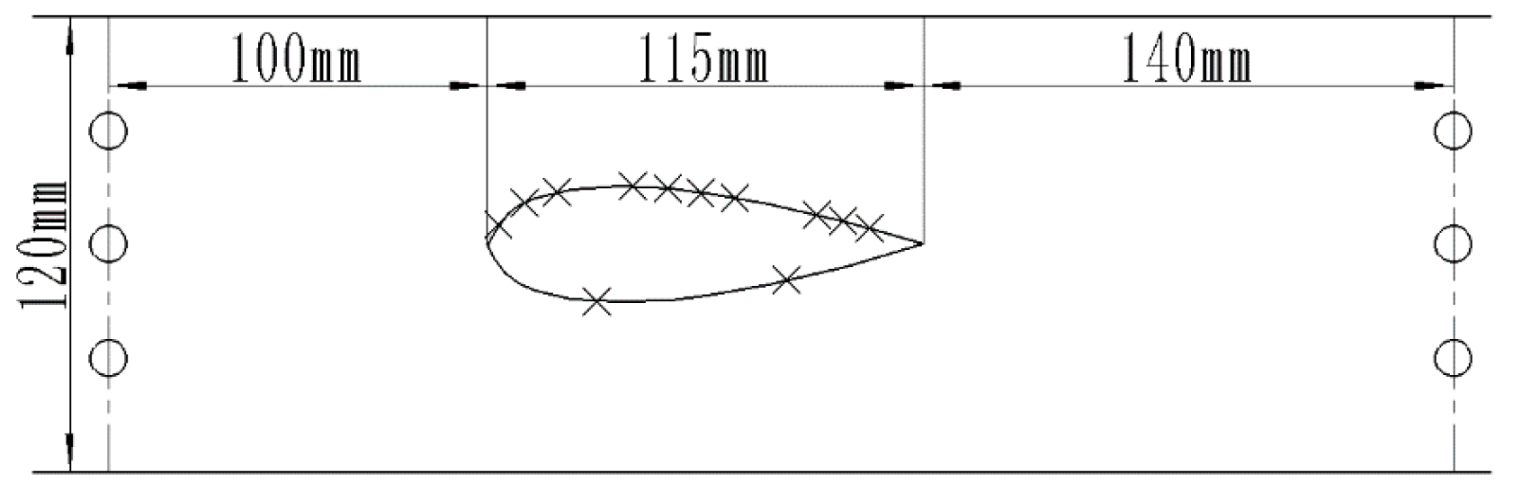
Figure 2.
3D model of the NACA0015 hydrofoil.
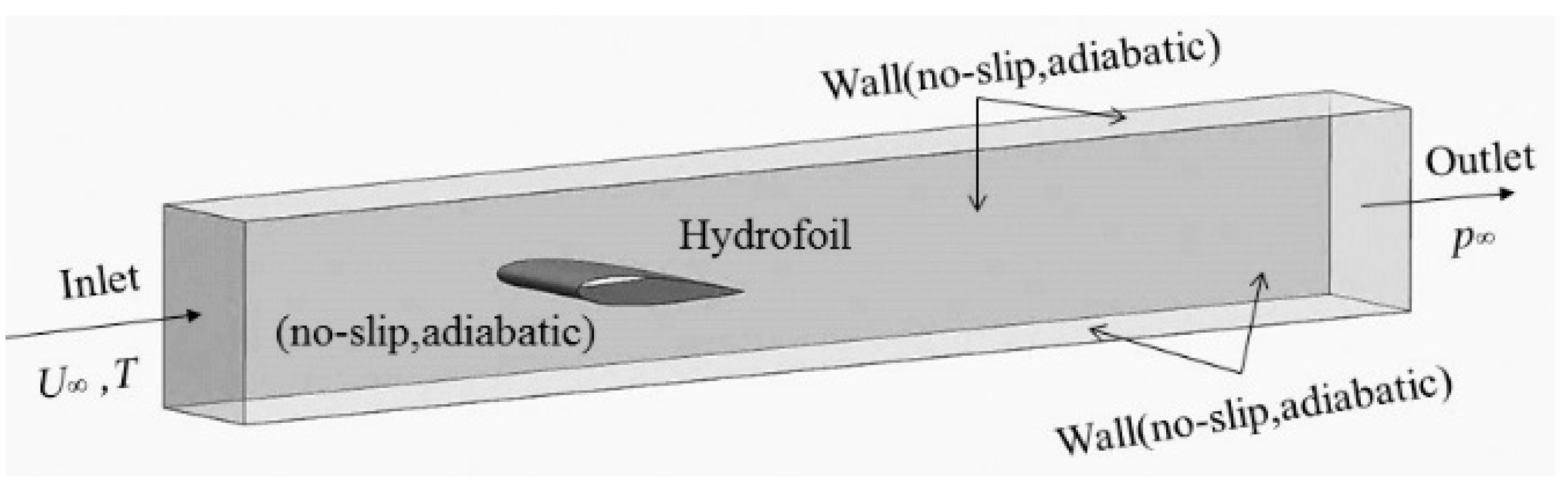
Figure 3.
Mesh implementation around the hydrofoil. (a) Mesh around leading edge, (b) Mesh around trailing edge.
Figure 3.
Mesh implementation around the hydrofoil. (a) Mesh around leading edge, (b) Mesh around trailing edge.
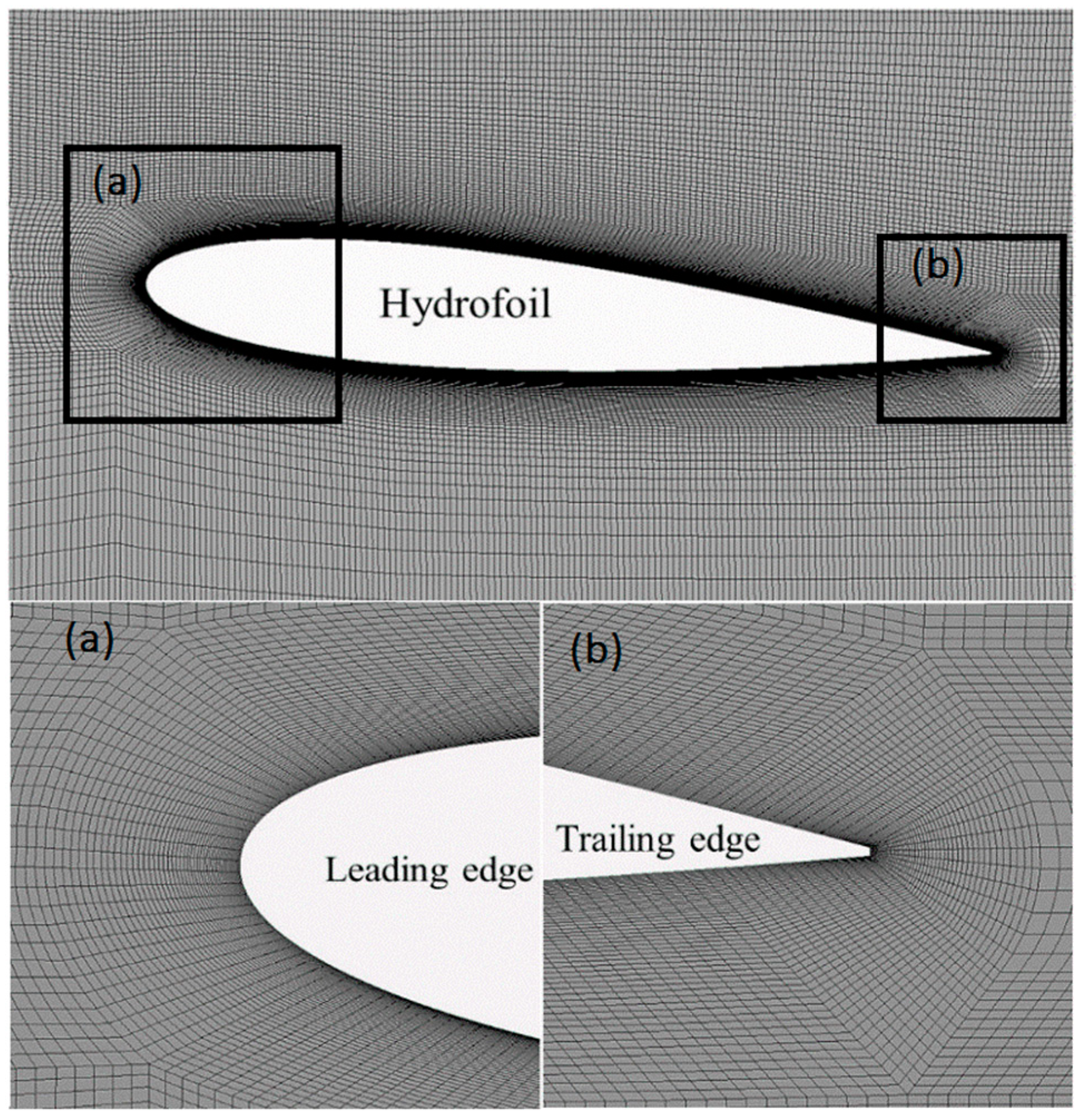
Figure 4.
y+ distribution along the upper surface and lower surface of the hydrofoil.

Figure 5.
Mesh independence study.

Figure 6.
Pressure coefficient distribution of the NACA0015 hydrofoil at 25 °C.
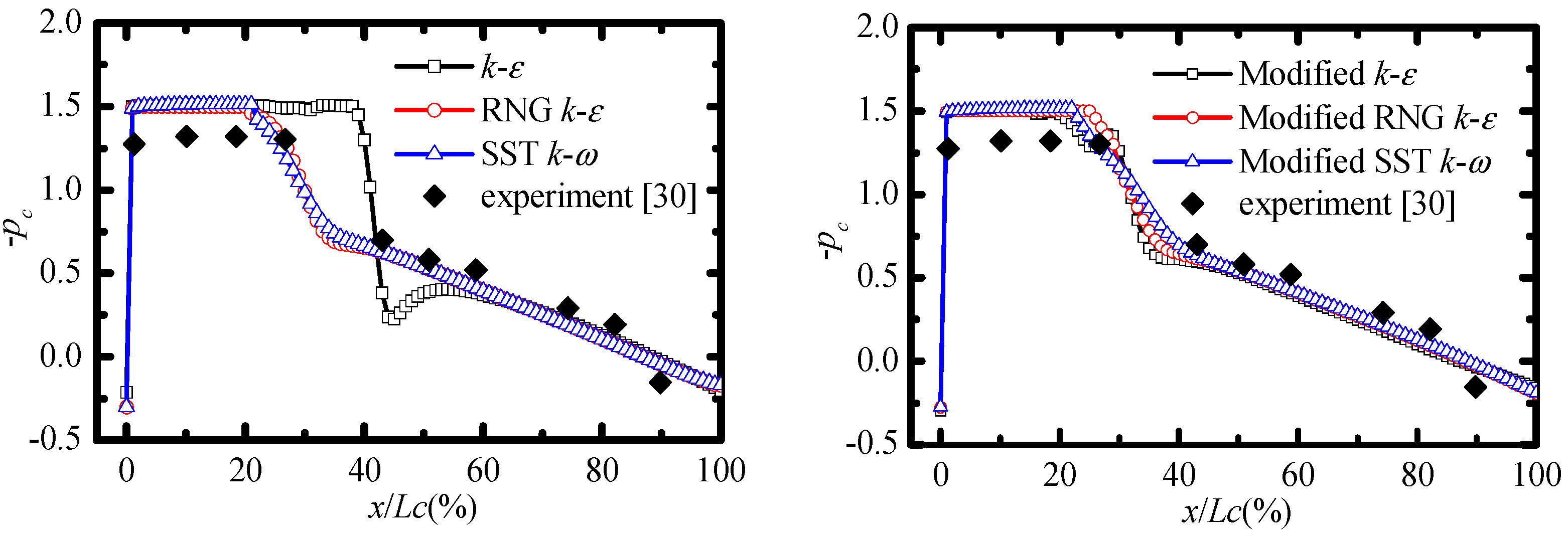
Figure 7.
Error analysis at 25 °C.
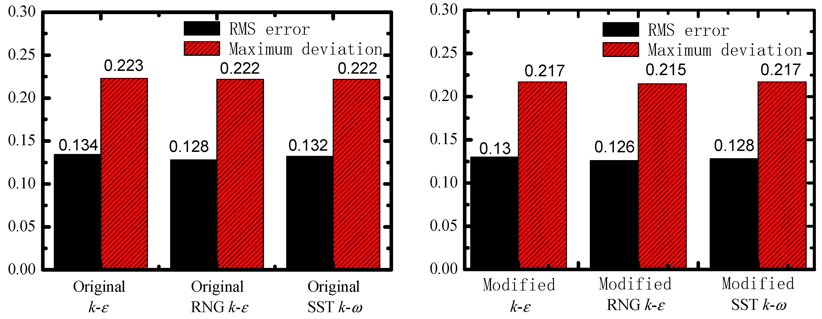
Figure 8.
Vapor volume fraction distribution on the surface of the NACA0015 hydrofoil.

Figure 9.
Pressure coefficient distribution of the NACA0015 hydrofoil at 50 °C.

Figure 10.
Error analysis at 50 °C.
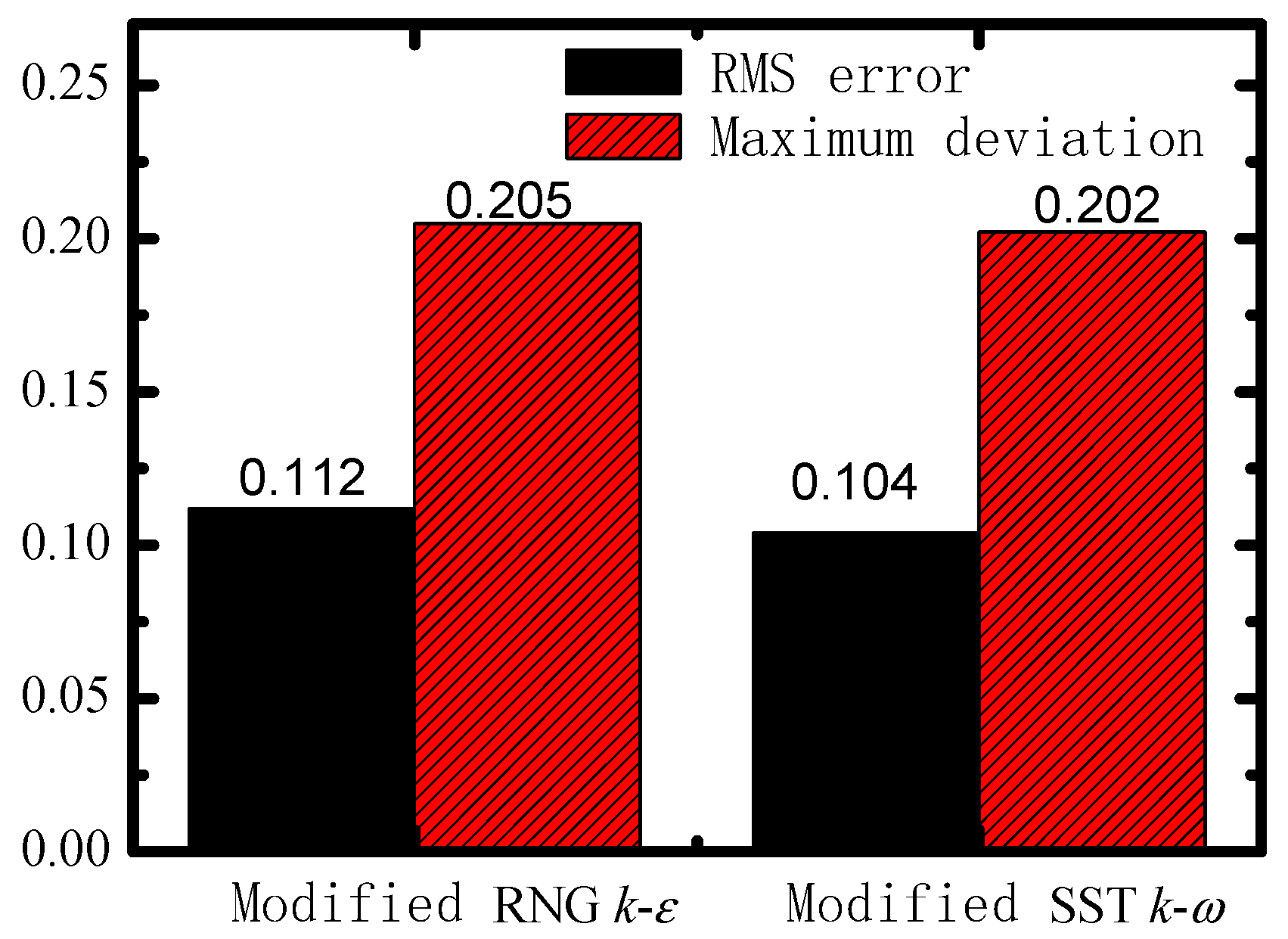
Figure 11.
Pressure coefficient distribution of the NACA0015 hydrofoil at 70 °C.
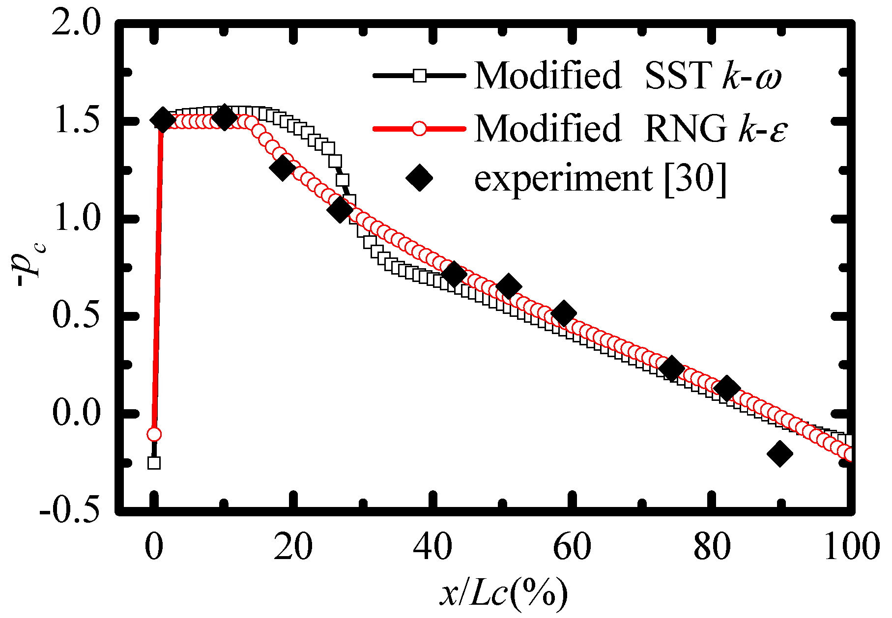
Figure 12.
Error analysis at 70 °C.
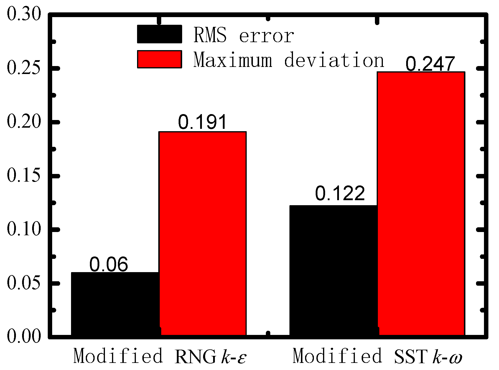
Figure 13.
Vapor volume fraction distribution on the surface of the NACA0015 hydrofoil.


Table 1.
Parameter setting at different temperatures.
| Fluid | Temperature T∞ (K) | Inlet Speed uin (m/s) | Outlet Pressure pout (Pa) |
|---|---|---|---|
| Water | 298 (25 °C) | 8 | 51,025 |
| Water | 323 (50 °C) | 8 | 59,768 |
| Water | 343 (70 °C) | 8 | 78,110.4 |
Table 2.
Mesh information.
| Mesh | Mesh Nodes | Min Angle | Max Aspect Ratio | Min Determinant | Min Quality |
|---|---|---|---|---|---|
| 1 | 1,138,840 | 46.08 | 145 | 0.794 | 0.72 |
| 2 | 2,847,100 | 46.08 | 56.1 | 0.794 | 0.72 |
| 3 | 4,555,360 | 46.08 | 34.8 | 0.794 | 0.72 |
© 2020 by the authors. Licensee MDPI, Basel, Switzerland. This article is an open access article distributed under the terms and conditions of the Creative Commons Attribution (CC BY) license (http://creativecommons.org/licenses/by/4.0/).
Share and Cite
MDPI and ACS Style
Deng, Y.; Feng, J.; Wan, F.; Shen, X.; Xu, B. Evaluation of the Turbulence Model Influence on the Numerical Simulation of Cavitating Flow with Emphasis on Temperature Effect. Processes 2020, 8, 997. https://doi.org/10.3390/pr8080997
AMA Style
Deng Y, Feng J, Wan F, Shen X, Xu B. Evaluation of the Turbulence Model Influence on the Numerical Simulation of Cavitating Flow with Emphasis on Temperature Effect. Processes. 2020; 8(8):997. https://doi.org/10.3390/pr8080997
Chicago/Turabian StyleDeng, Yilin, Jian Feng, Fulai Wan, Xi Shen, and Bin Xu. 2020. "Evaluation of the Turbulence Model Influence on the Numerical Simulation of Cavitating Flow with Emphasis on Temperature Effect" Processes 8, no. 8: 997. https://doi.org/10.3390/pr8080997
Note that from the first issue of 2016, this journal uses article numbers instead of page numbers. See further details here.