Article

Analysis of a Thermal Energy Storage Tank in a Large District Cooling System: A Case Study

Department of Mechanical Engineering, Universiti Teknologi PETRONAS, Seri Iskandar 32610, Perak, Malaysia
*
Author to whom correspondence should be addressed.
Processes 2020, 8(9), 1158; https://doi.org/10.3390/pr8091158
Submission received: 11 May 2020 / Revised: 14 July 2020 / Accepted: 20 July 2020 / Published: 16 September 2020
(This article belongs to the Section Energy Systems)

Abstract

:
This study’s primary goal is to evaluate the performance of a large thermal energy storage tank installed in a Gas District Cooling (GDC) plant. The performance parameters considered in this study include thermocline thickness (WTc), Cumulated Charge (Qcum), and Half Figure of Merit (½ FOM). The operation sensor data of a large Thermal Energy Storage (TES) tank was acquired for this analysis. The recorded temperature sensor from the 1st to 7th January and from 12th to 17th October 2019 was considered in this research. GraphPad prism computer software was deployed for analyses, and the temperature distribution data were analyzed to determine the four temperature parameters (hot water temperature (Th), cool water temperature (Tc), cool water depth (C), and slope gradient (S)) using a non-linear regression curve fitting technique and sigmoid Dose Responses function as integrated with the software. At the end of this research, the relationship between the growth of the determined performance parameter with charging hours was analyzed and presented. The research results proved the ability of GraphPad Prism software to assess the temperature distribution in the TES tank and also the corresponding effects on the overall Tank performance. The software offers better advantages in evaluating the performance parameter of the TES tank accurately.

1. Introduction

District Cooling System (DCS) is a smart solution that provides cooling energy within a centralized region. Thermal Energy Storage (TES) tank with Absorption Chillers (AC) and electrically driven Vapor Compression Chillers (VCC) are used to generate chilled water, which is transported to meet the substantial cooling demands for large spaces such as industrial facilities, universities, airports, and even residential areas [1]. The TES tank usage in GDC helps reduce capital cost, energy cost, carbon emissions, and equipment size, and makes for an improved chillers operation.
The help of the TES tank reduces the use of chillers during peak hours, thereby making it feasible for a higher chiller efficiency to be utilized, removing the disparity between demand and supply of energy [2,3]. In order to optimize energy saving and reduce the cost of TES operation, an optimal chiller plant strategy is developed [4]. In cases of increasing demand for refrigeration during peak hours, the additional chillers were switched over automatically [5].
Hasnain [6] reported that the most sophisticated and cost-efficient system in load management had been the resurgence of cool storage technology. The cooling system can be operated during off-peak night-time hours at low cooling loads using cold ambient temperature. Instead of using a compressor, cooling may be provided during the day at high peak by the circulation of the coolant medium [7].
The simplest form of cool TES makes use of chilled water as the storage medium [8]. TES tank has a distinct separation mechanism between cold and warm water, which is obtained either by providing physical barriers in tanks or by using natural stratification [9]. Physical barrier separation has been implemented with the labyrinth, baffle, and membrane based on the maze mechanism. In contrast, the natural process is achieved in thermally stratified systems, which permit the warm water to float on the top of cold water [10].
Naturally stratified tanks are less complicated, lower in cost, and equal or superior in thermal efficiency compared to other conventional forms of storage, making it a preferable option for TES designs [9]. Charging is done by introducing cool water into the lower nozzle, while warm water is removed from the upper nozzle of the TES tank [11]. Contrarily, discharging is carried out by the removal of cold water from the lower nozzle, while warm water is introduced from the upper nozzle. Both scenarios are pictorially explained in Figure 1.
In a stratified TES tank, warm water settles above cold water without any physical barrier. The separation of the two segments is preserved by the natural density difference between the warm water and cool water known as the thermocline.
Temperature distribution in the TES tank can be used to observe stratified TES tanks for several purposes. These include performance evaluations, parametric studies, and characterization of the determination of mixing effects [12]. The stratification of the TES tank enables cold water to distinctively settle in the bottom layer, while warm water occupies the upper layer of the TES tank, forming an S-curve demarcation where the thermocline is created. The boundary limit between cold and warm water volume is located at the midpoint of thermocline thickness known as the thermocline position C.
Various studies related to the analysis of temperature distribution of stratified TES tanks have been carried out by researchers. Temperature distribution can be used to determine various TES performance parameters [13].
Musser and Bahnfleth [11,14] used the temperature profile of a full-scale stratified chilled water TES tank for determining thermocline thickness at various charging and discharging flow rates. TES tank performance based on evaluating the half-cycle Figure of Merit was also conducted in the study. Musser and Bahnfleth [15] used a dimensionless cut-off temperature on each edge of the profile to bind the region in which most of the overall temperature change occurs. They suggested that the amount of the temperature profile to be discarded should be large enough to eliminate the effects of small temperature fluctuation at the thermocline’s extremes but small enough to capture most of the temperature change.
Bahnfleth, et al. [16] used temperature distribution to evaluate thermocline thickness on a full-scale stratified TES tank with slotted pipe diffuser.
Bahnfleth and Jing Song [17], in their study, researched the charging characterization of chilled water TES tank using a pair of ring octagonal slotted pipe diffusers in its configuration. This research was conducted at a constant flow rate. The initial temperature distribution was at a relatively uniform temperature after being fully discharged. In this research, the performance was quantified using thermocline thickness and a half-cycle Figure of Merit.
Walmsley et al. [18] used the siphoning method to manage thermocline thickness in an experimental stratified TES tank. The water temperature distribution was used to evaluate the effect of the re-established method on stratified TES tank operations. Joko [12], in his research, accurately determined the performance parameters of a hot stratified Thermal Energy Storage tank by using the temperature distribution profile of an operating TES tank. Joko’s analysis was based on a mathematical formulation that utilized the sigmoid Dose–Response equation. He concluded that the significant performance parameters, which include thermocline thickness, half-cycle Figure of Merit, and cumulative cooling capacity, could be accurately determined during the charging cycle of the TES tank. Majid et al. [19] analyzed in their study the thermal energy storage tank performance using thermocline thickness and half-cycle Figure of Merit. They obtained a temperature profile from simulating temperature as distributed in a TES tank by using a non-linear regression curve function and sigmoid Dose–Response. They concluded that based on the values they obtained on performance analysis the chilled water, TES Tank was undergoing degradation.
In this study, an approach for deriving the TES performance parameters, namely thermocline thickness, Half Figure of Merit, and the Accumulative Charge (Qcum), was established. GraphPad prism computer software was used to process the temperature distribution data using a non-linear regression technique to determine the hot water temperature (Th), cool water temperature (Tc), cool water depth (C), and slope gradient (S) parameter. These determined parameters representing the S-curve temperature profile were used to analyze the TES tank’s performance during the charging cycle [12,20]. Data used for the analysis in this research were acquired from a large district gas cooling plant with a remote sensor interval distance that records data every second. This study is a continuation of the research work outlined in the literature. The novelty of this research presents a computerized technique used to understand and compare the performance of a large full-scale TES tank over several months (10 months) of active operation. This study presents a unique and less ambiguous approach with a broader scope as compared to other related research.

System Overview

The GDC plant is installed with two TES tanks with a total holding capacity of 50,000 RTh (Refrigeration Ton-hour (RTh) is the of heat removal rate needed to freeze a metric ton (1000 kg) of water at 0 °C in 24 h) and the dimension of 24.5 m in diameter and 27.8 m in height. Data for analysis in this paper were taken from the daily operations of the Electric Chillers ECC and the TES tank as recorded.
In Figure 2, a block diagram represents the whole configuration of the Chiller plant as integrated into the District cooling plant operation. The set-up consists of four electric chillers, three cooling towers, and two air conditioners. The chillers’ heat is disposed of by the cooling towers as the chillers function to supply chilled water to charge the TES tank during low load periods.
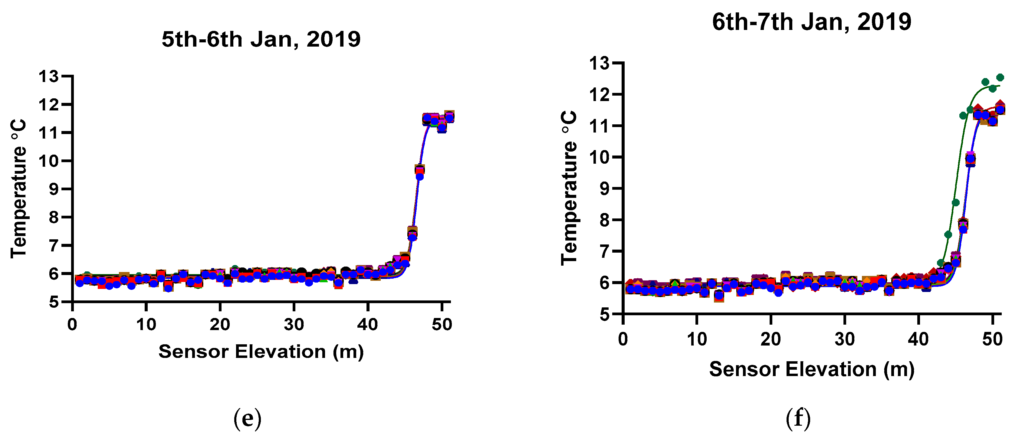
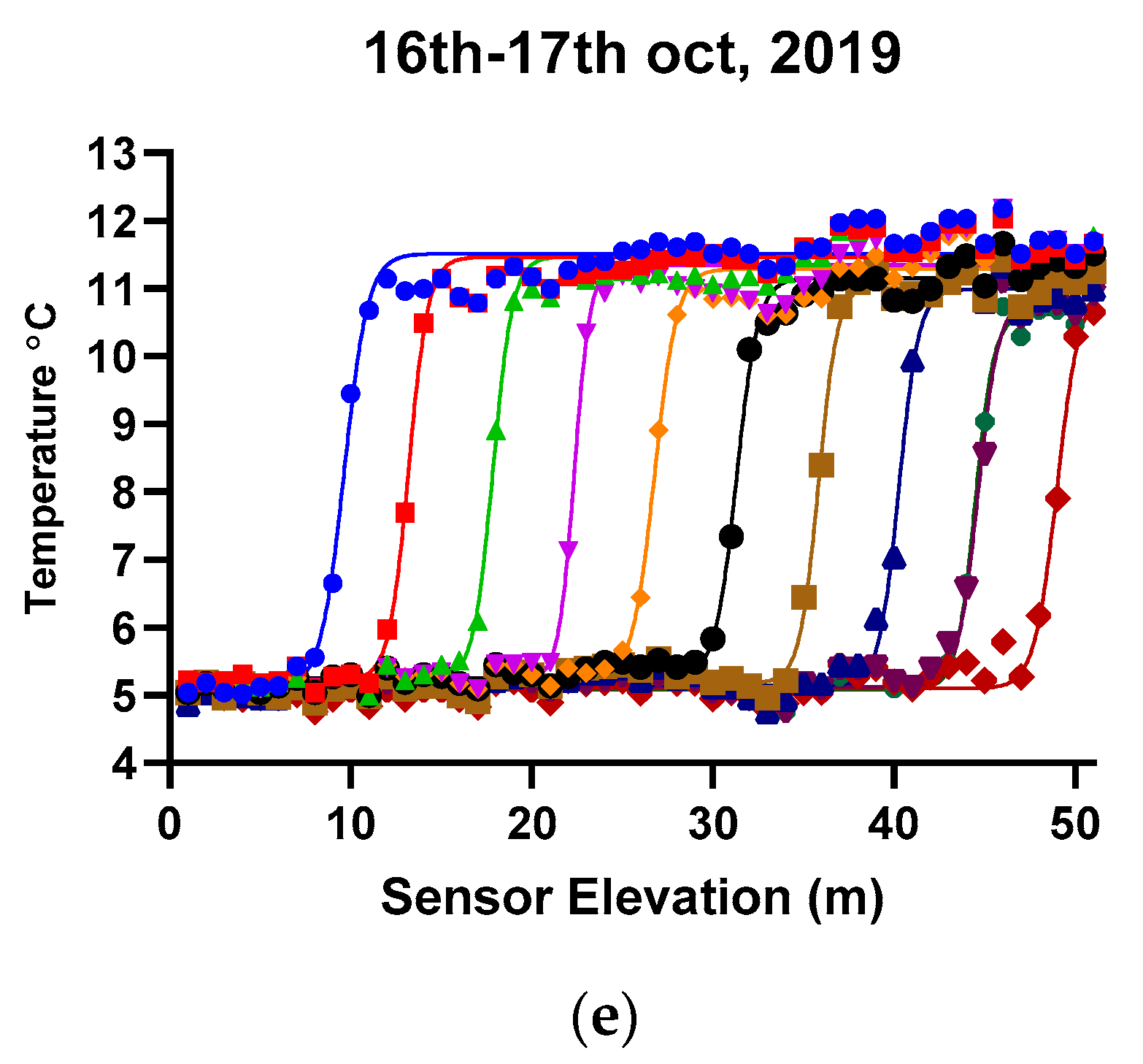
An hourly temperature dataset of the TES plant, from 1st to 7th January and from 12th to 15th October 2019, was used for the performance analysis. The data were used to obtain a temperature profile used in evaluating the performance parameters of the thermal storage tank. Performance parameters of the TES determined in this study include thermocline thickness, the half figure of performance, and cumulative cooling capacity.

2. Methodology

Usually, the water temperature distributional layout in the stratified TES tank is made up of 3 regions, namely,
  • warm water at the top (Th),
  • cold water at the bottom (Tc), and
  • thermocline region in the middle (WTc)
The water temperature profile forms an S-curved shape in which two asymptotes are present in its makeup. The average cold and warm water temperatures are formed by the asymptote values of the cold temperature (Tc) and hot temperature (Th) in the TES tank. The thermocline position (C) defines the boundary line between the cold Tc and warm Th fluid portion of the tank. Therefore, the region limited by the edges of the asymptote curve is referred to as Thermocline thickness.
Sigmoid Dose–Respond SDR function is denoted by Equation (1):
T(x) = T(C) + (Th − TC)/(1 + 10(C−X) S)
The GraphPad computer software uses the sigmoid Dose function technique in analyzing the temperature distribution to produce accurate values for function parameters (Tc, Th, C, and S).

2.1. Performance Parameters

The performance parameters analyzed in this study are thermocline thickness, half-cycle Figure of Merit (FOM) and accumulating charge capacity. These three parameters were employed in evaluating the performance of the TES tank of the DC plant.

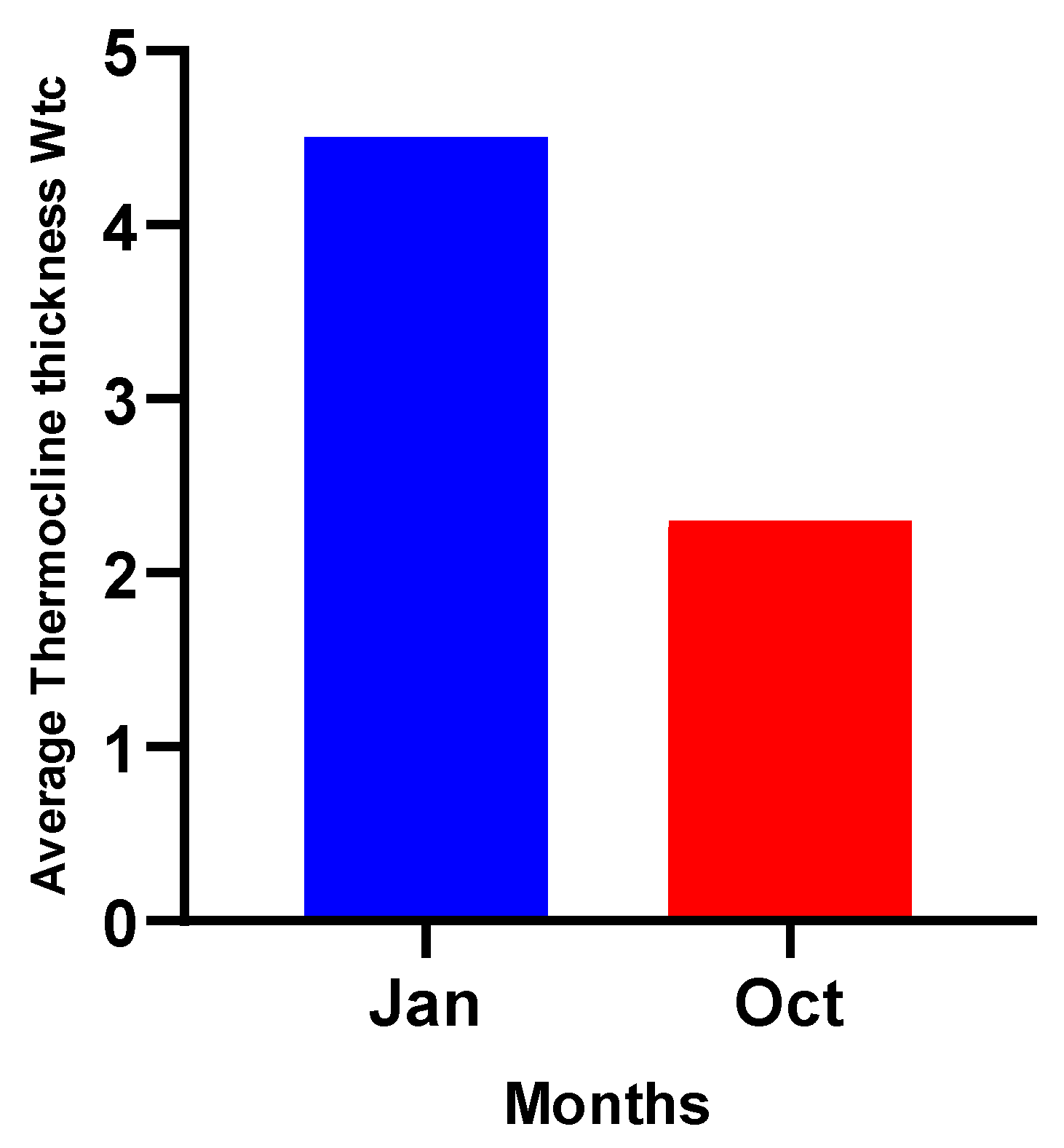
2.1.1. Determination of Thermocline thickness

Joko and Amin [21] formulated a mathematical relationship for determining thermocline thickness. Thermocline thickness was formulated based on the function relationship by identifying the function of the temperature profile. The concept for determining thermocline thickness was achieved by rearranging the equation into the form;
Th Tc T Tc = 1 + 10 ( c x ) s
Using dimensionless cut-off temperature in Equation (3)
Ө   =   ( T Tc ) ( Th Tc )
Re-arranging and stating the limit point of the thermocline thickness Equation (4) is derived;
1 Ө = 1 + 10 ( c x ) s
From Equation (4), making C − X the subject of formulae, we have;
C X = log ( 1 Ө 1 ) S
Distance from C to X denotes half the thermocline thickness;
C X = W t c 2
Therefore, from Equations (5) and (6), thermocline thickness can be expressed as;
W t c = ( log (   1 Ө 1 ) S )
Musser, A. and W.P. Bahnfleth [11] established that the dimensionless cut-off ratio Ө values range from 0 to 0.5, covering minimum and maximum thermocline thickness. Ө = 0 indicates that the thermocline edges profile is located at Tc, and Th therefore gives a maximum thickness. With Ө = 0.5, the limit points are at the midpoint of the thermocline region, resulting in zero values of the thickness. Moreover, with Ө equal to 0 and 0.5, it revealed ∞ and 0, respectively. The mixing area measured from its edge is known as the thermocline thickness. The edge of the thermocline is referred to as dimensionless cut-off temperature Ө stated in Equation (3).

2.1.2. Determination of Half Figure of Merit FOM

Figure of Merit (FOM) is the ratio of integrated discharge capacity for a given volume to the ideal capacity that could have been achieved without mixing and losses to the environment. Although FOM seems straightforward in its definition, it may be challenging to evaluate its parameter in the field because most chilled water storage cannot perform full cycle tests spanning for 24 h or longer. It is therefore desirable to analyze the “half-cycle” performance of tanks over Half Figure of Merit. Half FOM is consequently defined as the ratio of integrated capacity (capacity useful energy stored in TES tank) to the theoretical capacity (capacity of cooling energy stored in the absence of losses) [15].
Half FOM is given as
½   F O M   =   Cint Cmax
where
C i n t = A . ρ . C p . ( Th Tc ) S   ( log ( 1 + 10 s c )     log 2 )
C m a x = ρ . A . C p . C ( Th Tc )
Therefore,
Closs = CmaxCint

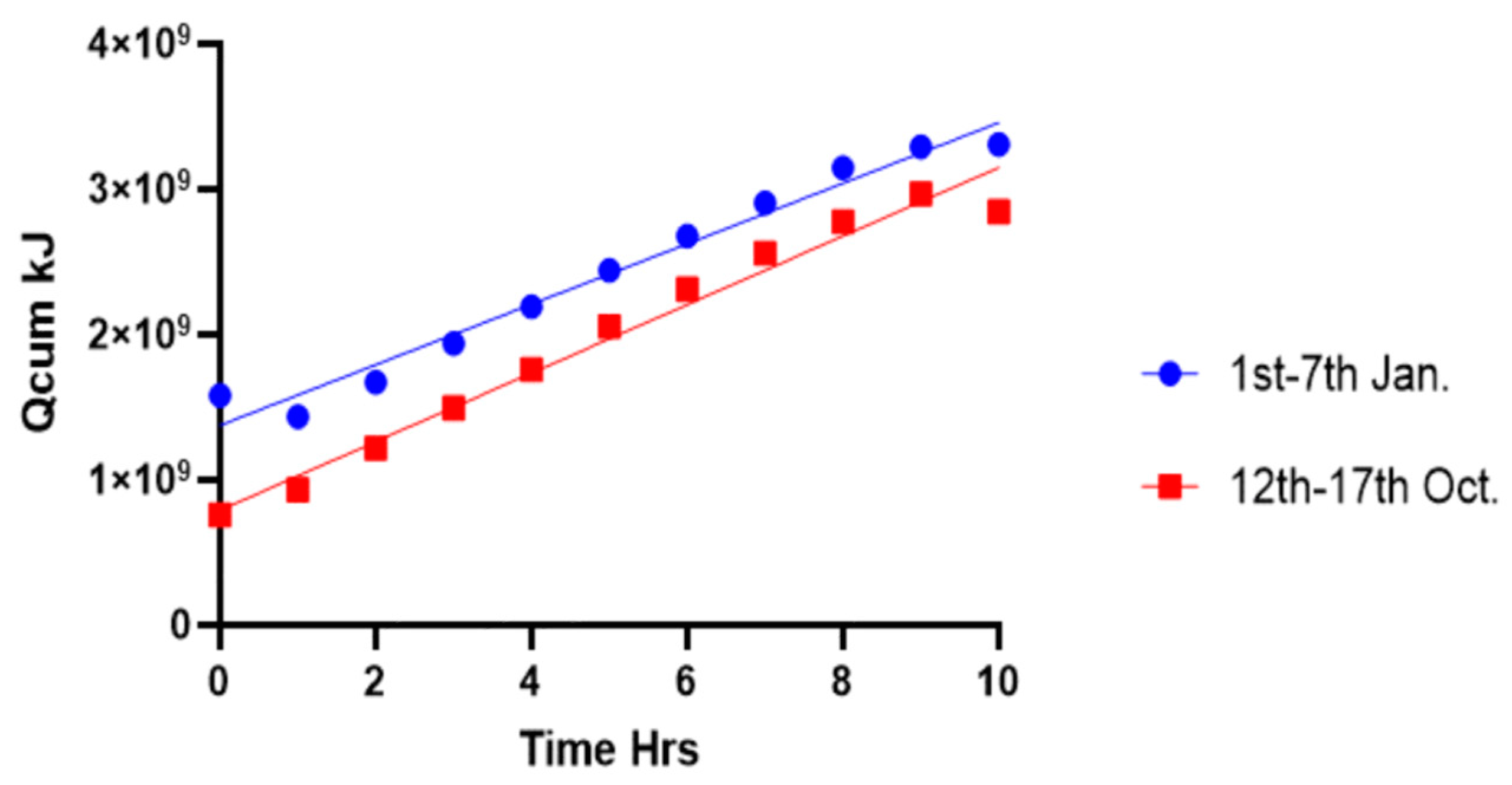
2.1.3. Determination of Cumulative Cooling Capacity Qcum

This describes the capacity of stored energy during the charging cycle of a stratified thermal storage tank. Joko Waluyo [12] in his research formulated a mathematical expression (in Equation (12)) to calculate the cumulative cooling capacity of a TES tank.
Q c u m = A . ρ . C p . ( Th Tc ) S ( log ( 1 + 10 s c )     log ( 1 + 10 S ( C H ) ) )
  • where A = Area of circular Tank (m2)
  • ρ = Water density (kg/m3) and
  • Cp is the specific heat of the water at average temperature (kJ/kg °C).

3. Results and Discussion

3.1. Data Acquisition

The data acquired comprise readings of tank datasheets, daily production reports, and the temperature for every layer in the stratified thermal energy storage tank. Data on the TES tank specification and the plant operations were extracted from the datasheet. Temperature distribution and the holding capacity of thermal energy storage were also extracted from the daily TES tank report for January 2019 to October 2019, while for the data of the production of the chilled water were taken from the daily electrical chiller report for January 2019 to October 2019. Table A1 presented in Appendix A shows a sample of the temperature distribution data for the 1st–2nd January 2019.

3.2. Plotting the Temperature Distribution on GraphPad Prism Software (Fitting Profile of Temperature Distribution)

Curve fitting was employed to find the set of parameter values of the function that best approaches the collected data. This thus minimizes the deviation between the observed and expected temperature values of each sensor. For this purpose, the commercial software GraphPad prism was used for its analysis. Hourly plots of different times of the year (1st–7th January to 12th–19th October 2019), which represent the fitting profile of the temperature distribution of the charging cycle, were analyzed on the software and are presented in Figure 3a–f and Figure 4a–f.
GraphPad Prism visual plots in Figure 3 and Figure 4 show that the temperature distribution is well fitted, and it followed a regular charging trend. Streams of charge on every hour assumed the S-curve shape on every instance as charging starts from 10 p.m. and ends at 8 a.m. each day.

3.3. Obtaining Curve Fitting and Performance Parameters

After plotting the temperature distribution profile, the metric that best fits the function would then be determined. In this study, parameters Tc, Th, C, and S were generated using the commercial software GraphPad Prism 8. Table 1 and Table A2, Table A3, Table A4, Table A5 and Table A6 contain parameter data from 1st to 7th January 2019, while Table A7, Table A8, Table A9, Table A10, Table A11 and Table A12 contain parameter data from 12th to 17th October 2019. Table A2, Table A3, Table A4, Table A5, Table A6, Table A7, Table A8, Table A9, Table A10, Table A11 and Table A12 are presented in Appendix A.
The parameter data analysis, as presented in Table 1 and Table A2, Table A3, Table A4, Table A5, Table A6, Table A7, Table A8, Table A9, Table A10, Table A11 and Table A12, provides complete information regarding curve fitting temperature parameters and the performance parameter during the hourly charging cycle of the TES tank. The coefficient of determination R2 reveals that the correlation between experimental and obtained values in the curve fitting evaluation is well fitted as they all approached the value 1.
Figure 5 shows the plot of the average thermocline position C as against the charging time. As displayed on the chart, the result reveals that the position of thermocline changes with respect to hours of charging, as charging of the thermal energy storage tank proceeds the position of thermocline tends to move upward from the bottom of the tank until charging ends.
For thermocline thickness WTC evaluation, the growth of thermocline thickness with charging time is revealed in Table 1 and Table A2, Table A3, Table A4, Table A5, Table A6, Table A7, Table A8, Table A9, Table A10, Table A11 and Table A12, with the dimensionless cut-off temperature Ө set at 0.1.
The overall results, as shown in Figure 6 and Table 1 and Table A2, Table A3, Table A4, Table A5, Table A6, Table A7, Table A8, Table A9, Table A10, Table A11 and Table A12, revealed that thermocline thickness was mostly constant throughout the charging time. The maximum thermocline thickness was observed at the lower part of the storage tank as a result of the position near the inlet diffuser, where the mixing has a more substantial influence. As the thermocline position moves further away from the inlet diffuser towards the top, improved quality of thermocline was recorded during charging. This was a result of the reduced mixing that occurred within the tank as the cold mixture moves towards the outlet diffuser. The average thermocline thickness from 1st–7th January was 4.5 m and from 12th–17th October was 2.3 m; this means a 48.9% decrease in thermocline thickness between these months, as revealed in Figure 7. This means there was improved performance of the TES plant in terms of the thermocline.
Results, as shown in Figure 8, reveal that charging started at 10 p.m. and ended at 8 a.m. The cumulative charge was observed to increase with the charging duration. It is also worthy to note that the average cumulative charge capacity (Qcum) dropped between these months as presented in Figure 9. There was a 16.9% drop in the average cumulative charge from January to October 2019 in the TES performance operation.
The result, as shown in Figure 10, reveals that ½ FOM increased as the charging process was initiated as suggested in past literature [12,15,22], and it assumed a steady value (near 1) moments into the charging process. This scenario occurs due to the decrease in the thermocline thickness as the thermocline position C moves upwards towards the top of the stratified TES tank where there is less mixing of cold and warm regions of fluids. Figure 11 reveals that the average half FOM as evaluated from 1st to 7th January was 0.96, and from 12th to 17th October was 0.98. This means that there was a 2.16% increase in the average half FOM in between these months, showing improved performance of the TES tank operation. This implies that the thermal efficiency of the tank improved as there was less conduction loss and mixing occurring in the tank during operation.
Based on the result, a higher temperature difference between the hot and cold regions of the tank makes for a thinner thermocline thickness, thereby improving the efficiency of the tank. Since temperature distribution is significantly affected as a result of mixing near the inlet nozzles [11,13], it is recommended that the designers install appropriate and more efficient diffusers at the nozzle connection [11].
This research further provides keen insight on TES operations for researchers, designers, and maintenance experts. It helps relate the temperature distribution trend in a large full-scale TES tank with various performance parameters over time. This approach provides practitioners with just enough information necessary to understand the internal workings of a large full-scale TES system based on the output temperature sensor readings at each time of operation.

4. Conclusions

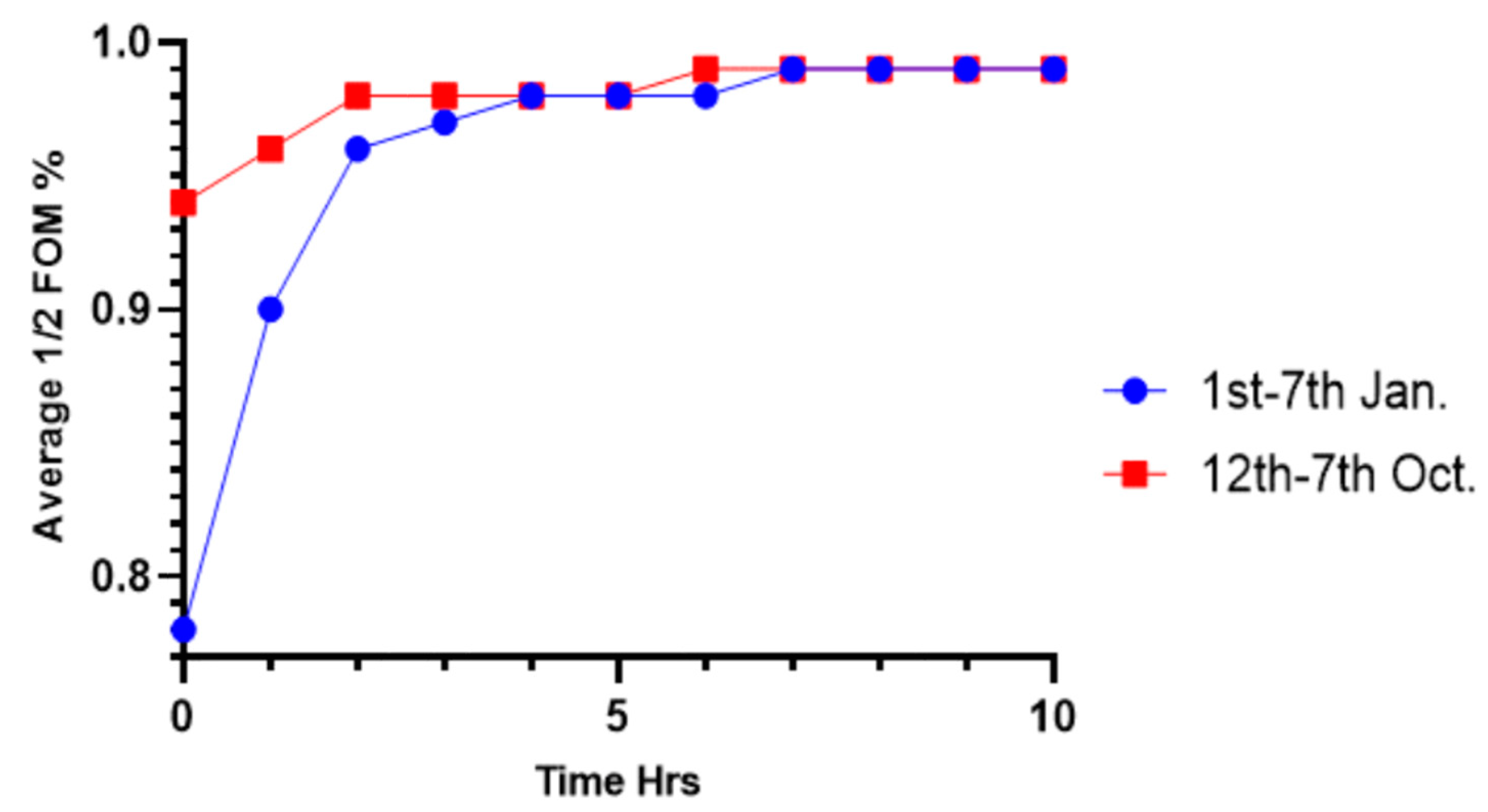
Data from the operation of a full-scale Large District Cooling Plant were used for this study. Hourly temperature readings of 51 sensors as installed in the TES tank were acquired for analysis. The charging cycle from 1st to 7th January and from the 12th to 17th October 2019 was used in this analysis and comparison. GraphPad prism computer software was deployed for processing and analyzing the temperature distribution data using a non-linear regression curve fitting technique and a sigmoid Dose–Responses SDR function to determine the four-temperature parameter, namely hot water temperature (Th), cool water temperature (Tc), cool water depth (C), and slope gradient (S). These four parameters were used to determine the performance parameters (WTc, ½ FOM, and Qcum) of the TES tank through established mathematical formulations. Based on the values of the average thermocline thickness and Half Figure of Merit from the results, it was observed that the stratified chilled water TES tank experienced an upgrade in its performance from the month of January to October 2019. Analysis of the operation of the plant revealed that there was a 48.9% decrease in the average thermocline thickness and a 2.16% increase on the average half FOM for the period of January through October 2019. This reveals that the stratified TES tank experienced an upgrade in its performance efficiency. This upgrade might have resulted from an improved general operation of the DGC plant or the replacement or servicing of components like the chillers. It can be suggested that the decrease in thermocline thickness may be as a result of less mixing in the hot and cold region of the fluid, thereby improving the quality of stored energy in the TES tank. The substantial decrease of thermocline thickness led to an increase in the tank’s half FOM because a thinner thermocline thickness translates to the less fluid mixture in the stratified tank, which results in a higher 1/2 FOM.
Based on the result, it can be concluded that GraphPad Prism software provides a less ambiguous technique with less computational time in understanding the behavior of the temperature profile of a full-scale TES tank at any time of operation.
The characterization of various performance parameters based on the behavior of the temperature profile as revealed in this research will further provide designers, maintenance experts, and researchers more useful insight on the working of a large TES plant during its charging cycle. It helps relate the temperature distribution trend in a large full-scale TES tank with various performance parameters over time. Although the scope of this research is broader in terms of TES size and the time considered in performance comparison, the conclusion made correlates with findings in other literature work that made use of various techniques in understanding the temperature distribution in the TES tank.

Author Contributions

M.A.A.M.: Supervision, methodology, and revision. M.M.: Data acquisition and revision. C.C.H.: Main manuscript drafting, data analysis, conceptualization and editing. A.B.A.: Supervision. All authors have read and agreed to the published version of the manuscript.

Funding

Authors wish to acknowledge Universiti Teknologi PETRONAS for support of this research and financial support of (British Council) Grant cost centre 015ME-015 for this research.

Conflicts of Interest

The authors declare no conflict of interest.

Nomenclatures

SymbolsDescriptionUnits
CThermocline position m
CintIntegrated capacitykJ
ClostLost capacitykJ
CmaxTheoretical capacitykJ
CpSpecific heat of waterkJ
FoMFigure of Merit%
½ FoMHalf Figure of Merit%
HTank water depthm
QcumCumulative charge kJ
SSlope of GradientDimensionless
TcCold water temperature°C
ThHot water temperature°C
WTcThermocline thicknessm
Greek Symbols Units
ӨDimensionless temperature Dimensionless
ρDensitykg/m3
AbbreviationDescription
ACAbsorption Chiller
ECCElectric Chiller
GDCGas District Cooling
HVACHeat Vapour Air Conditioning
RThRefrigeration Ton-hour
VCCVapour Compression Chiller

Appendix A

Table A1. Sample of Sensor temperature Readings in a DC plant (for 1st–2nd October 2019).
Temperatures (°C) at Various Charging Time
Sensor Elevation22:00 p.m.0:00 a.m.2:00 a.m.4:00 a.m.6:00 a.m.8:00 a.m.
5111.5411.6911.6211.6911.149.12
5011.6411.6411.6611.6411.129.06
4911.5911.5811.5411.5810.556.92
4811.5611.7111.611.567.615.35
4711.0911.1911.1611.035.745.04
4611.4311.4511.4711.255.565.4
4511.2511.3711.2911.095.355.22
4411.4411.511.4411.255.485.4
4311.2811.2911.2710.915.45.22
4211.4311.4311.4311.095.45.23
4111.1511.211.1410.725.125.09
4011.6111.5811.5310.915.45.22
3911.5111.5411.438.165.225.08
3811.5811.5811.46.085.225.22
3711.4511.4511.125.435.095.09
3611.6411.6411.35.435.355.07
3511.6411.6411.35.385.35.08
3411.4811.4811.125.25.124.94
3311.4811.4811.095.135.124.99
3211.611.6111.15.35.175.06
3111.1211.1110.554.914.964.73
3011.6111.619.875.195.275.19
2911.3511.26.615.075.074.88
2811.5811.35.775.135.225.06
2711.5111.25.455.145.174.99
2611.3211.045.1955.074.94
2511.6411.225.435.255.35.08
2411.6411.125.435.255.385.23
2311.6411.125.435.255.35.12
2211.3510.865.145.15.154.96
2110.8810.034.74.644.684.61
2010.946.654.754.754.764.75
1910.765.534.864.684.74.7
1810.64.914.734.674.584.55
1710.654.944.784.784.784.78
1610.654.944.784.74.714.66
1510.424.834.74.584.74.65
1410.654.944.784.784.784.78
1310.64.794.784.784.784.78
1210.424.834.74.74.734.7
118.414.784.784.624.684.62
106.314.944.934.834.844.78
95.144.814.814.814.834.78
84.834.654.654.654.684.56
74.684.684.684.684.74.68
64.84.664.574.624.574.62
55.014.874.784.834.784.83
44.934.84.684.814.684.62
34.934.864.684.814.854.75
24.884.814.624.74.624.7
14.74.624.624.74.624.56
Table A2. 2nd–3rd January 2019 Curve Fitting and Performance Parameter analysis.
HoursӨTh (°C)Tc (°C)C(m)SR2WtcQcum (kJ)½ FOM
22:000.110.089.885~11.75~27480.1059---
23:000.110.095.7323.0551.1630.95511.64101.72 × 1080.915308
0:000.110.085.5137.3581.5880.98591.20184.34 × 1080.974237
1:000.110.125.32511.52.1750.99230.87757.13 × 1080.987965
2:000.110.095.20616.171.0590.99231.80221.02 × 1090.982421
3:000.110.095.15120.551.1490.99451.66101.31 × 1090.987251
4:000.110.065.16625.171.3340.99271.43061.59 × 1090.991035
5:000.110.055.14629.61.050.99381.81761.88 × 1090.990314
6:000.110.185.16734.261.2620.99471.51232.22 × 1090.993038
7:000.110.025.0938.531.1230.99371.69952.45 × 1090.993043
8:000.110.235.11540.331.0630.99081.79542.67 × 1090.992978
Table A3. 3rd–4th January 2019 Curve Fitting and Performance Parameter analysis.
HoursӨTh (°C)Tc (°C)C(m)SR2WtcQcum (kJ)½ FOM
22:000.111.665.1648.7970.28420.9686.71537.39 × 1080.880141
23:000.111.635.39611.590.29630.9766.44119.34 × 1080.912388
0:000.111.575.33915.970.31510.97916.05681.29 × 1090.940179
1:000.111.415.33920.470.40090.98334.76051.61 × 1090.963318
2:000.111.275.3324.710.50430.98473.78441.9 × 1090.975843
3:000.111.395.27129.550.26130.98527.30382.34 × 1090.961014
4:000.111.065.31433.830.56560.98993.37432.51 × 1090.984267
5:000.110.985.25638.150.58650.98883.25402.82 × 1090.986546
6:000.110.655.25542.461.0460.98281.82462.96 × 1090.993222
7:000.110.245.22246.940.5770.96933.30763.04 × 1090.988885
8:000.110.95.16547.320.95850.98021.99113.51 × 1090.993363
Table A4. 4th–5th January 2019 Curve Fitting and Performance Parameter analysis.
HoursӨTh (°C)Tc (°C)C (m)SR2WtcQcum (kJ)½ FOM
22:000.111.545.1519.870.67190.99442.84048.15 × 1080.954607
23:000.111.615.21613.430.65020.99372.93521.11 × 1090.965526
0:000.111.615.20418.090.93470.99562.04181.5 × 1090.982197
1:000.111.515.14522.620.72240.99582.64191.86 × 1090.981578
2:000.111.465.17427.10.83820.99312.27692.2 × 1090.986748
3:000.111.535.11831.60.64340.99592.96622.62 × 1090.985194
4:000.111.515.11336.040.85080.99672.24322.98 × 1090.990183
5:000.111.385.11940.540.67740.99512.81743.28 × 1090.989038
6:000.111.275.13444.810.60970.98983.13023.55 × 1090.988982
7:000.110.955.10648.990.85350.97452.23613.7 × 1090.992801
8:000.110.715.06645.231.3220.98741.44363.3 × 1090.994966
Table A5. 5th–6th January 2019 Curve Fitting and Performance Parameter analysis.
HoursӨTh (°C)Tc (°C)C (m)SR2WtcQcum (kJ)½ FOM
22:000.111.515.1029.6350.66430.98362.87297.98 × 1080.952968
23:000.111.465.22113.190.80070.99092.38351.06 × 1090.971497
0:000.111.475.21317.850.80190.99022.38001.44 × 1090.978969
1:000.111.345.23322.340.99460.99041.91881.76 × 1090.986452
2:000.111.295.23726.770.70570.99122.70442.09 × 1090.984065
3:000.111.155.25531.290.73610.99482.59272.38 × 1090.98693
4:000.111.075.17735.830.82620.99542.31002.73 × 1090.989831
5:000.110.995.14140.270.79120.99322.41213.04 × 1090.990552
6:000.110.845.12144.630.76950.98942.48023.3 × 1090.991235
7:000.111.025.09648.990.69650.97022.74013.75 × 1090.991178
8:000.110.625.08644.480.84650.99282.25463.18 × 1090.992005
Table A6. 6th–7th January 2019 Curve Fitting and Performance Parameter analysis.
HoursӨTh (°C) Tc (°C)C (m)SR2WtcQcum (kJ)½ FOM
22:000.111.515.28.3291.3810.99051.38206.79 × 1080.973829
23:000.111.475.25612.531.6560.98971.15251.01 × 1090.985492
0:000.111.475.1916.961.10.991.73501.38 × 1090.983864
1:000.111.455.16321.621.0690.991.78531.76 × 1090.986975
2:000.111.335.15925.991.0770.99021.77202.07 × 1090.989246
3:000.111.295.18730.531.4120.98961.35162.41 × 1090.993017
4:000.111.35.15535.051.1320.98891.68592.78 × 1090.992413
5:000.111.125.14439.481.4150.99111.34883.05 × 1090.994611
6:000.111.025.10643.81.0320.98971.84933.35 × 1090.99334
7:000.110.875.11148.41.1830.98941.61333.6 × 1090.994742
8:000.110.125.11548.442.0520.99150.93013.13 × 1090.996971
Table A7. 12th–13th October 2019 Curve Fitting and Performance Parameter analysis.
HoursӨTh (°C) Tc (°C)C (m)SR2WtcQcum (kJ)½ FOM
22:000.110.415.21212.380.85510.99412.23198.32 × 1080.971564
23:000.110.395.40714.011.0180.99451.87479.02 × 1080.978893
0:000.110.375.2618.770.9840.99591.93951.24 × 1090.983701
1:000.110.375.23224.081.0580.99461.80391.6 × 1090.988184
2:000.110.345.17228.980.78940.99322.41761.94 × 1090.986841
3:000.110.385.21633.980.85910.99182.22152.27 × 1090.989688
4:000.110.385.174390.75270.98812.53552.62 × 1090.989745
5:000.110.265.159440.89330.98632.13642.9 × 1090.992341
6:000.110.435.22549.260.7290.93312.61793.31 × 1090.991617
7:000.1~19135.022~91.630.077860.786224.5118--
8:000.110.825.10447.70.86410.97562.20863.52 × 1090.992697
Table A8. 13th–14th October 2019 Curve Fitting and Performance Parameter analysis.
HoursӨTh (°C) Tc (°C)C (m)SR2WtcQcum (kJ)½ FOM (%)
22:000.111.2411.0817.59~55.240.2325---
23:000.111.245.6371.350.31790.9136.00341.29 × 1080.618802
0:000.111.296.5026.5070.36450.98245.23594.03 × 1080.873856
1:000.111.345.50910.930.30560.99386.24508.24 × 1080.909936
2:000.111.35.26715.710.29350.99516.50251.22 × 1090.934715
3:000.111.35.1820.730.2820.99556.76771.64 × 1090.948506
4:000.111.35.16825.690.2830.9966.74382.04 × 1090.958594
5:000.111.315.14730.650.2670.99517.14792.44 × 1090.963215
6:000.111.265.14135.840.2710.99347.04242.83 × 1090.969006
7:000.111.235.16540.10.29040.99196.57193.14 × 1090.97415
8:000.111.215.16637.190.28280.9956.74852.9 × 1090.971378
Table A9. 14th–15th October 2019 Curve Fitting and Performance Parameter analysis.
HoursӨTh (°C) Tc (°C)C (m)SR2WtcQcum (kJ)½ FOM
22:000.111.878.424-0.85780.074590.824225.58631.61 × 1080.481601
23:000.111.726.2376.0260.57450.96833.32204.27 × 1080.913089
0:000.111.765.84210.90.51590.98383.69938.34 × 1080.946468
1:000.111.735.67715.650.51930.99123.67511.22 × 1090.962959
2:000.111.695.65620.920.60960.99373.13071.63 × 1090.976395
3:000.111.685.63225.820.53050.99363.59752.02 × 1090.978023
4:000.111.555.62930.850.57410.99343.32432.36 × 1090.983003
5:000.111.455.59836.040.66390.99362.87472.73 × 1090.987419
6:000.111.315.57640.840.61980.99063.07923.03 × 1090.988108
7:000.111.195.50644.480.57140.98043.34003.27 × 1090.988156
8:000.111.435.55241.630.61990.98693.07873.16 × 1090.988335
Table A10. 15th–16th October 2019 Curve Fitting and Performance Parameter analysis.
HoursӨThTcCSR2WtcQcum (KJ)½ FOM
22:000.111.878.424-0.85780.074590.824225.58631.61 × 1080.481601
23:000.111.726.2376.0260.57450.96833.32204.27 × 1080.913089
0:000.111.765.84210.90.51590.98383.69938.34 × 1080.946468
1:000.111.735.67715.650.51930.99123.67511.22 × 1090.962959
2:000.111.695.65620.920.60960.99373.13071.63 × 1090.976395
3:000.111.685.63225.820.53050.99363.59752.02 × 1090.978023
4:000.111.555.62930.850.57410.99343.32432.36 × 1090.983003
5:000.111.455.59836.040.66390.99362.87472.73 × 1090.987419
6:000.111.315.57640.840.61980.99063.07923.03 × 1090.988108
7:000.111.195.50644.480.57140.98043.34003.27 × 1090.988156
8:000.111.435.55241.630.61990.98693.07873.16 × 1090.988335
Table A11. 16th–17th October 2019 Curve Fitting and Performance Parameter analysis.
HoursӨTh (°C) Tc (°C)C (m)SR2WtcQcum (kJ)½ FOM
22:000.111.55.83746.60.76490.98782.49513.41 × 1090.991555
23:000.111.525.86346.560.76110.98942.50753.4 × 1090.991505
0:000.111.525.88346.560.74780.98752.55213.39 × 1090.991354
1:000.111.65.88846.560.73620.98772.59233.44 × 1090.991218
2:000.111.585.8946.580.75360.98852.53253.42 × 1090.991424
3:000.111.565.92246.550.73470.98812.59763.39 × 1090.991198
4:000.111.585.90446.510.69240.98942.75633.41 × 1090.990652
5:000.111.435.90846.520.81130.99082.35243.32 × 1090.992024
6:000.111.595.9146.510.71650.98932.66363.41 × 1090.990967
7:000.111.565.90946.520.73630.98932.59203.4 × 1090.991211
8:000.111.625.94846.570.71380.98882.67373.41 × 1090.990944
Table A12. 18th–19th October 2019 Curve Fitting and Performance Parameter analysis.
HoursӨTh (°C) Tc (°C)C (m)SR2WtcQcum (kJ)½ FOM
22:000.111.455.88146.360.67080.99052.84513.34 × 1090.99032
23:000.111.455.89746.380.67260.98972.83753.33 × 1090.99035
0:000.111.475.92146.340.63650.992.99843.32 × 1090.989794
1:000.111.455.91446.310.65390.992.91863.31 × 1090.990059
2:000.111.435.9346.340.67560.99022.82493.29 × 1090.990385
3:000.111.475.92646.320.6240.98963.05853.32 × 1090.989585
4:000.111.415.9446.320.65960.98892.89343.27 × 1090.990147
5:000.111.465.93546.370.64370.99112.96493.31 × 1090.989915
6:000.111.465.98946.320.62550.98973.05113.27 × 1090.98961
7:000.111.615.96846.330.6020.98943.17023.38 × 1090.989207
8:000.112.285.95745.040.49340.99153.86803.68 × 1090.986454

References

  1. Sarbu, I.; Sebarchievici, C. A comprehensive review of thermal energy storage. Sustainability 2018, 10, 191. [Google Scholar] [CrossRef] [Green Version]
  2. Tay, N.; Liu, M.; Belusko, M.; Bruno, F. Review on transportable phase change material in thermal energy storage systems. Renew. Sustain. Energy Rev. 2017, 75, 264–277. [Google Scholar] [CrossRef]
  3. Wu, Y.; Chen, C.; Jia, Y.; Wu, J.; Huang, Y.; Wang, L. Review on electrospun ultrafine phase change fibers (PCFs) for thermal energy storage. Appl. Energy 2018, 210, 167–181. [Google Scholar] [CrossRef]
  4. Kapoor, K.; Powell, K.M.; Cole, W.J.; Kim, J.S.; Edgar, T.F. Improved large-scale process cooling operation through energy optimization. Processes 2013, 1, 312–329. [Google Scholar] [CrossRef] [Green Version]
  5. Yau, Y.; Rismanchi, B. A review on cool thermal storage technologies and operating strategies. Renew. Sustain. Energy Rev. 2012, 16, 787–797. [Google Scholar] [CrossRef]
  6. Hasnain, S.M. Review on sustainable thermal energy storage technologies, Part I: Heat storage materials and techniques. Energy Convers. Manag. 1998, 39, 1127–1138. [Google Scholar] [CrossRef]
  7. Chen, S.-L.; Chen, C.L.; Tin, C.C.; Lee, T.S.; Ke, M.C. An experimental investigation of cold storage in an encapsulated thermal storage tank. Exp. Therm. Fluid Sci. 2000, 23, 133–144. [Google Scholar] [CrossRef]
  8. Rutberg, M.; Hastbacka, M.; Cooperman, A.; Bouza, A. Thermal energy storage. ASHRAE J. 2013, 55, 62. [Google Scholar]
  9. Karim, A.; Burnett, A.; Fawzia, S. Investigation of stratified thermal storage tank performance for heating and cooling applications. Energies 2018, 11, 1049. [Google Scholar] [CrossRef] [Green Version]
  10. Alva, G.; Lin, Y.; Fang, G. An overview of thermal energy storage systems. Energy 2018, 144, 341–378. [Google Scholar] [CrossRef]
  11. Musser, A.; Bahnfleth, W.P. Field-Measured performance of four full-scale cylindrical stratified chilled-water thermal storage tanks. ASHRAE Trans. 1999, 105, 218. [Google Scholar]
  12. Waluyo, J. Determination of Performance Parameters of Hot Stratified Thermal Energy Storage Tank. In Proceedings of the 2016 6th International Annual Engineering Seminar, Yogyakarta, Indonesia, 1–3 August 2016. [Google Scholar]
  13. Waluyo, J.W. Simulation Models for Single and Two-Stage Charging of Stratified Thermal Energy Storage. Ph.D. Thesis, Universiti Teknologi Petronas, Seri Iskandar, Malaysia, 5 June 2012. [Google Scholar]
  14. Musser, A.; Bahnfleth, W.P. Evolution of temperature distributions in a full-scale stratified chilled-water storage tank with radial diffusers. ASHRAE Trans. 1998, 104, 55. [Google Scholar]
  15. Bahnfleth, W.P.; Musser, A. Thermal performance of a full-scale stratified chilled-water thermal storage tank. Trans. Am. Soc. Heat. Refrig. Air Cond. Eng. 1998, 104, 377–388. [Google Scholar]
  16. Bahnfleth, W.P.; Song, J.; Cimbala, J.M. Measured and modeled charging of a stratified chilled water thermal storage tank with slotted pipe diffusers. HVAC R Res. 2003, 9, 467–491. [Google Scholar] [CrossRef]
  17. Bahnfleth, W.P.; Song, J. Constant flow rate charging characteristics of a full-scale stratified chilled water storage tank with double-ring slotted pipe diffusers. Appl. Therm. Eng. 2005, 25, 3067–3082. [Google Scholar] [CrossRef]
  18. Walmsley, M.R.; Atkins, M.J.; Riley, J. Thermocline Management of Stratified Tanks for Heat Storage; AIDIC Servizi S.r.l.: Rome, Italy, 2009; pp. 231–236. [Google Scholar]
  19. Majid, M.A.A.; Yamin, M.F. Study on the performance analysis of stratified thermal energy storage system of a district cooling plant. In AIP Conference Proceedings; AIP Publishing LLC: Seri Iskandar, Malaysia, 2018. [Google Scholar]
  20. Karim, M. Performance evaluation of a stratified chilled-water thermal storage system. World Acad. Sci. Eng. Technol. 2009, 53, 326–334. [Google Scholar]
  21. Waluyo, J.; Majid, M.A.A.; Amin, M. Temperature profile and thermocline thickness evaluation of a stratified thermal energy storage tank. Int. J. Mech. Mechatron. Eng. 2010, 1, 7–12. [Google Scholar]
  22. Majid, M.A.A.; Nasir, M.; Waluyo, J. Operation and performance of a thermal energy storage system: A case study of campus cooling using cogeneration plant. Energy Procedia 2012, 14, 1280–1285. [Google Scholar] [CrossRef] [Green Version]
Figure 1. Charging and discharging scenario in the Thermal Energy Storage (TES) tank: (a) Charging, (b) Discharging.
Processes 08 01158 g001
Figure 2. Configuration of 4 chillers at a large Gas District Cooling plant using the block diagram.
Processes 08 01158 g002
Figure 3. Temperature distribution plot for 1st–7th of January 2019 on GraphPad prism software (af).
Processes 08 01158 g003aProcesses 08 01158 g003b
Figure 4. Temperature distribution plot for 12th–17th of October 2019 on GraphPad prism software (ae).
Processes 08 01158 g004aProcesses 08 01158 g004b
Figure 5. Average Thermocline Position (C) with Time.
Processes 08 01158 g005
Figure 6. Average thermocline thickness (WTc) with time.
Processes 08 01158 g006
Figure 7. Average thermocline thickness trend between January and October 2019.
Processes 08 01158 g007
Figure 8. Average cumulative charge over time.
Processes 08 01158 g008
Figure 9. Average cumulative charge with month.
Processes 08 01158 g009
Figure 10. The plot of average Half Figure of Merit (½ FOM) with charging hours.
Processes 08 01158 g010
Figure 11. The average ½ FOM trend between January and October 2019.
Processes 08 01158 g011
Table 1. 1st–2nd January 2019 Curve Fitting and Performance Parameter analysis.
HoursӨTh (°C) Tc (°C)C (m)SR2WtcQcum (kJ)½ FOM
22:000.110.315.557~22.11~5.4420.9921---
23:000.110.275.55421.342.0360.99230.93741.3 × 1090.993072
0:000.110.245.57621.111.5590.99131.22421.27 × 1090.990853
1:000.110.235.59121.31.9550.99120.97621.28 × 1090.992771
2:000.110.225.544210.90770.99272.10261.27 × 1090.984208
3:000.110.255.59321.182.3580.99150.80941.27 × 1090.993972
4:000.110.275.58821.141.0280.99221.85651.28 × 1090.986148
5:000.110.255.55521.051.030.99181.85291.28 × 1090.986116
6:000.110.265.58521.181.7710.99171.07761.28 × 1090.991975
7:000.110.215.56721.21.5920.99241.19881.27 × 1090.991081
8:000.110.245.56521.211.4840.99281.28601.28 × 1090.990436

