
Numerical Prediction of Homogeneity of Gas Flow through Perforated Plates


Abstract
:1. Introduction
2. Previous Studies of Modelling of Flow through Perforated Plates
3. Materials, Methods and Procedure
3.1. Modelling Approach
3.2. Validation Apparatus and Procedure
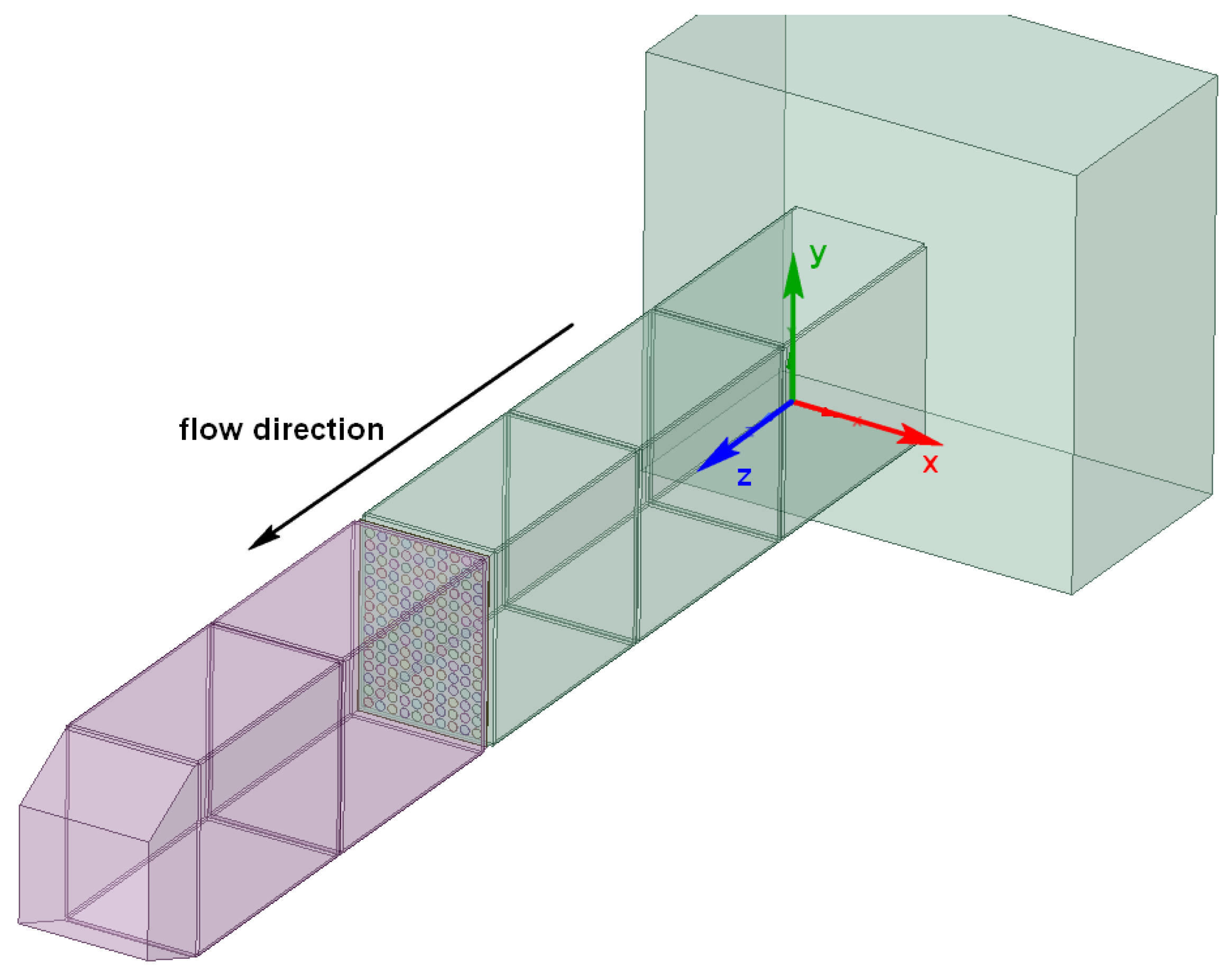
3.2.1. The Testing Stand
3.2.2. Single Plate Modelling
- the flow was at the steady state condition;
- air was treated as an incompressible gas of density 1.225 kg/m3;
- air is free from ash, dust, or any other particles;
- there was no presence of electrostatic field or other acting sources, except gravitational force;
- temperature of air does not change.
3.2.3. Experimental Validation
4. Results of Modelling of the Panels
4.1. Modelling of the Perforated Plates with Different Open Area Ratios
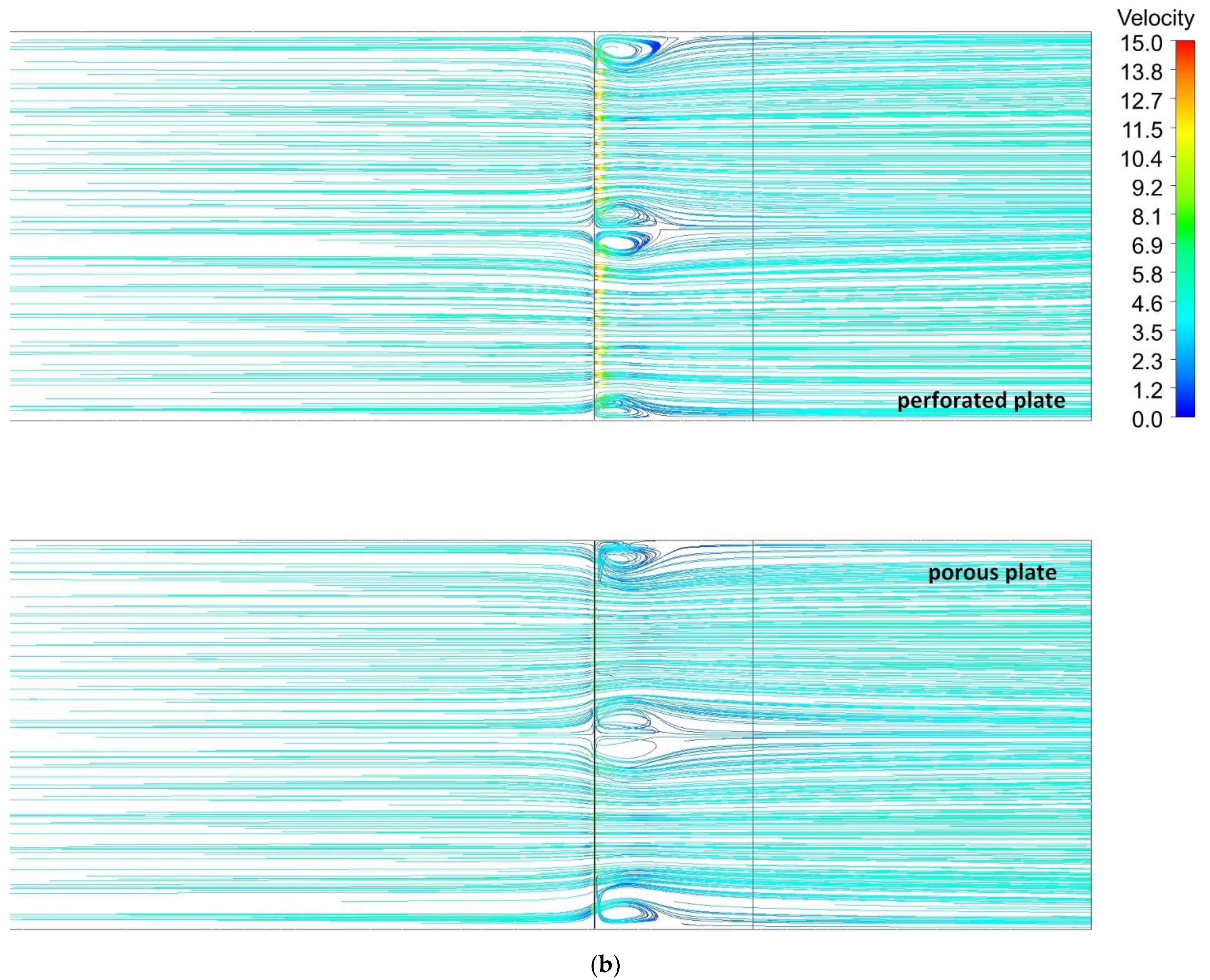
4.2. Modelling of Single Porous Plate
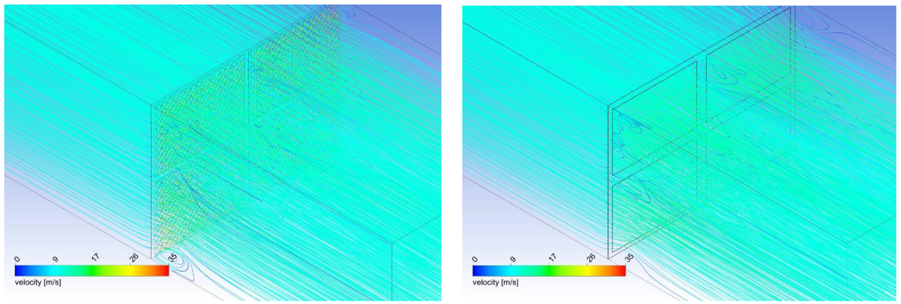
4.3. Modelling of Test Panel Plate
5. Conclusions
- The paper presents the approach of the modelling of flow through such complex objects as large-scale perforated plates using the porous core model. The proposed method can be interesting and easy to apply by engineers for designing and optimising complex structures in which structural elements cannot be ignored. An example of such a structure is an ESP used in power technology.
- The proposed numerical modelling approach predicts well the air flow through the perforated plates of different open area ratios with use of the porous model. This can lead to a significant reduction in time and required computational resources for the design and modelling of the flow where homogeneity is required.
- Pressure drop through the perforated plate obtained from a CFD simulation fits the experimental pressure drop with an error less than 1%. Pressure drop of the plates of the different open area ratios can be approximated by the mean of polynomial functions.
- Proposed correlation can be used for prediction of the internal resistance coefficient as a function of the plate open area ratio. The pressure drop through the porous core predicted by simulations using developed correlation differs from the pressure drop generated by a perforated plate by less than 20%.
- Qualitative and quantitative obtained results in terms of velocity field and pressure drop across the plate show that the proposed approach has great potential for practical applications. As the next step, investigations into angular flow through the plates are proposed. This would allow the area of application of the proposed approach to be increased. In addition, the application of apparent porosity instead of the actual porosity may be investigated to further improve the proposed method.
Author Contributions
Funding
Institutional Review Board Statement
Informed Consent Statement
Data Availability Statement
Acknowledgments
Conflicts of Interest
Nomenclature
| AO, AC | surface area of holes, total surface area of the plate, respectively, m2 |
| C2 | internal resistant coefficient, m−1 |
| D | diameter, m |
| f | open area ratio of the plate, |
| p | pressure, Pa |
| P | porosity, |
| u | velocity, m/s |
| α | permeability, m2 |
| δ | thickness of the plate, m |
| ρ | density, kg/m3 |
| μ | dynamic air viscosity, Pa∙s |
References
- Pistoresi, C.; Fan, Y.; Luo, L. Numerical study on the improvement of flow distribution uniformity among parallel mini-channels. Chem. Eng. Process. Process Intensif. 2015, 95, 63–71. [Google Scholar] [CrossRef] [Green Version]
- Mazur, M.; Bhatelia, T.; Kuan, B.; Patel, J.; Webley, P.A.; Brandt, M.; Pareek, V.; Utikar, R. Additively manufactured, highly-uniform flow distributor for process intensification. Chem. Eng. Process. Process Intensif. 2019, 143, 107595. [Google Scholar] [CrossRef]
- Govindan, B.; Jakka, S.C.B.; Radhakrishnan, T.K.; Saashi, K.G.N.; Tiwari, A.K.; Manoj, K.S.; Tulsyan, P.; Kalburgi, A.K.; Balasubramanya, H.A. CFD approach in design of effective distributor for uniform dispersion of cohesive ultrafine particles in a downer reactor. Chem. Eng. Process. Process Intensif. 2020, 157, 108138. [Google Scholar] [CrossRef]
- Miller, B.G. Advanced flue gas dedusting systems and filters for ash and particulate emissions control in power plants. In Woodhead Publishing Series in Energy: Advanced Power Plant Materials, Design and Technology; Dermot Roddy, D., Ed.; Woodhead Publishing: Sawston, UK, 2010; pp. 217–243. [Google Scholar]
- European Parliament. Commission Implementing Decision (EU) 2017/1442 of 31 July 2017 under Directive 2010/75/EU. 2017. Available online: EUR-Lex-32017D1442-EN-EUR-Lex(europa.eu) (accessed on 27 September 2021).
- Swaminathan, M.R.; and Mahalakshimi, M.W. Numerical modelling of flow though perforated plates applied to electrostatic precipitators. J. Appl. Sci. 2010, 10, 2426–2432. [Google Scholar] [CrossRef]
- The Institute of Clean Air Companies (1997), Electrostatic Precipitator Gas Flow Model Studies (rev. 2004) Guidelines for Modeling Gas Flows in Electrostatic Precipitators in Order to Ensure Flow Uniformity in the Finished Unit. Publication ICAC EP-7, Electronic Document. Available online: https://cdn.ymaws.com/www.icac.com/resource/resmgr/Standards_WhitePapers/EP7_final.pdf (accessed on 27 September 2021).
- Xu, Y.; Deng, B.; Zhang, H.; Chen, X. Numerical simulation of electrostatic field and flow field in an electro-static precipitator. J. Air Pollut. Health 2019, 4, 87–98. [Google Scholar] [CrossRef]
- Kaiser, S.; Fahlenkamp, H. CFD Modelling of the Electrical Phenomena and the Particle Precipitation Process of Wet ESP in Coaxial Wire-tube Configuration. Int. J. Plasma Environ. Sci. Technol. 2011, 5, 103–109. [Google Scholar]
- Heidarbeig, M.; Mohebbi, A. CFD Modeling of Particulate Pollutants Removal by Electrostatic Precipitator (ESP). In Proceedings of the 8th International Chemical Engineering Congress & Exhibition (IChEC 2014), Kish, Iran, 24–27 February 2014. [Google Scholar]
- Haque, S.M.E.; Rasul, M.G.; Khan, M.M.K.; Deev, A.V.; Subaschandar, N. A Numerical Model of an Electrostatic Precipitator. In Proceedings of the 16th Australasian Fluid Mechanics Conference, Gold Coast, Australia, 3–7 December 2007; pp. 1050–1054. [Google Scholar]
- Scodras, G.; Kaldis, S.P.; Sofialidis, D.; Faltsi, O.; Grammelis, P.; Sakellaropoulos, G.P. Particulate removal via electrostatic precipitators—CFD simulation. Fuel Process. Technol. 2006, 87, 623–631. [Google Scholar] [CrossRef]
- Arif, S.; Branken, D.J.; Everson, R.C.; Neomagus, H.W.J.P.; le Grange, L.A.; Arif, A. CFD modeling of particle charging and collection in electrostatic precipitators. J. Electrost. 2016, 84, 10–22. [Google Scholar] [CrossRef]
- Guo, B.Y.; Hou, Q.F.; Yu, A.B.; Li, L.F.; Guo, J. Numerical modelling of the gas flow through perforated plates. Chem. Eng. Res. Des. 2013, 91, 403–408. [Google Scholar] [CrossRef]
- Yusop, A.F.; Mamat, R.; Mat Yasin, M.H.; Suhaimi, S. Effects of the Inlet Velocity Profiles on the Prediction of Velocity Distribution inside an Electrostatic Precipitator. Int. J. Comput. Electr. Eng. 2014, 6, 64–66. [Google Scholar] [CrossRef]
- Kouropoulos, G. Two-Dimensional Computational Simulation Flow Of Exhaust Gases Passing Inside An Electrostatic Precipitator. J. Urban Environ. Eng. 2018, 10, 106–112. [Google Scholar] [CrossRef]
- Celik, N.; Bayazit, Y.; Turgut, E.; Sparrow, E.M. Design Analysis Of Fluid-Flow Through Perforated Plates. Therm. Sci. 2018, 22, 3091–3098. [Google Scholar] [CrossRef] [Green Version]
- Haque, S.M.E.; Rasul, M.G.; Deev, A.; Khan, M.M.K.; Zhou, J. The influence of flow distribution on the performance improvement of electrostatic precipitator. In Proceedings of the 10th International Conference on Electrostatic Precipitation (ICESP), Cairns, Australia, 26–27 June 2006. Paper No. 2A1. [Google Scholar]
- Haque, S.M.E.; Rasul, M.G.; Deev, A.; Khan, M.M.K.; Subaschandar, N. Flow simulation in an electrostatic precipitator of a thermal Power plant. Appl. Therm. Eng. 2009, 29, 2037–2042. [Google Scholar] [CrossRef]
- ANSYS Fluent User Guide, Release 14.0; ANSYS, Inc.: Canonsburg, PA, USA, 2011.
- Butrymowicz, D.; Śliwiński, Ł.; Śmierciew, K.; Karwacki, J.; Ochrymiuk, T.; Lackowski, M.; Przybyliński, T.; Antes, T. Indirect method of numerical modelling of perforated plates in electrostatic precipitators. In Proceedings of the 12th International Conference on Boiler Technology ICBT 2014, Szczyrk, Poland, 21–24 October 2014; pp. 111–123. [Google Scholar]
- Hou, Q.F.; Guo, B.Y.; Li, L.F.; Yu, A.B. Numerical Simulation of Gas Flow in An Electrostatic Precipitator. In Proceedings of the 7th International Conference on CFD in the Minerals and Process Industries, CSIRO, Melbourne, Australia, 9–11 December 2009. [Google Scholar]


| Procedure, Type of Studies | Effect | |
|---|---|---|
| 1 | Initial numerical studies of single plate, f = 0.30 | estimation of the flow disturbances |
| 2 | experimental investigation of single plate, f = 0.40 | experimental results database: pressure drop, velocity distribution |
| 3 | numerical studies of single plate, f = 0.40 | numerical results database: pressure drop, velocity distribution |
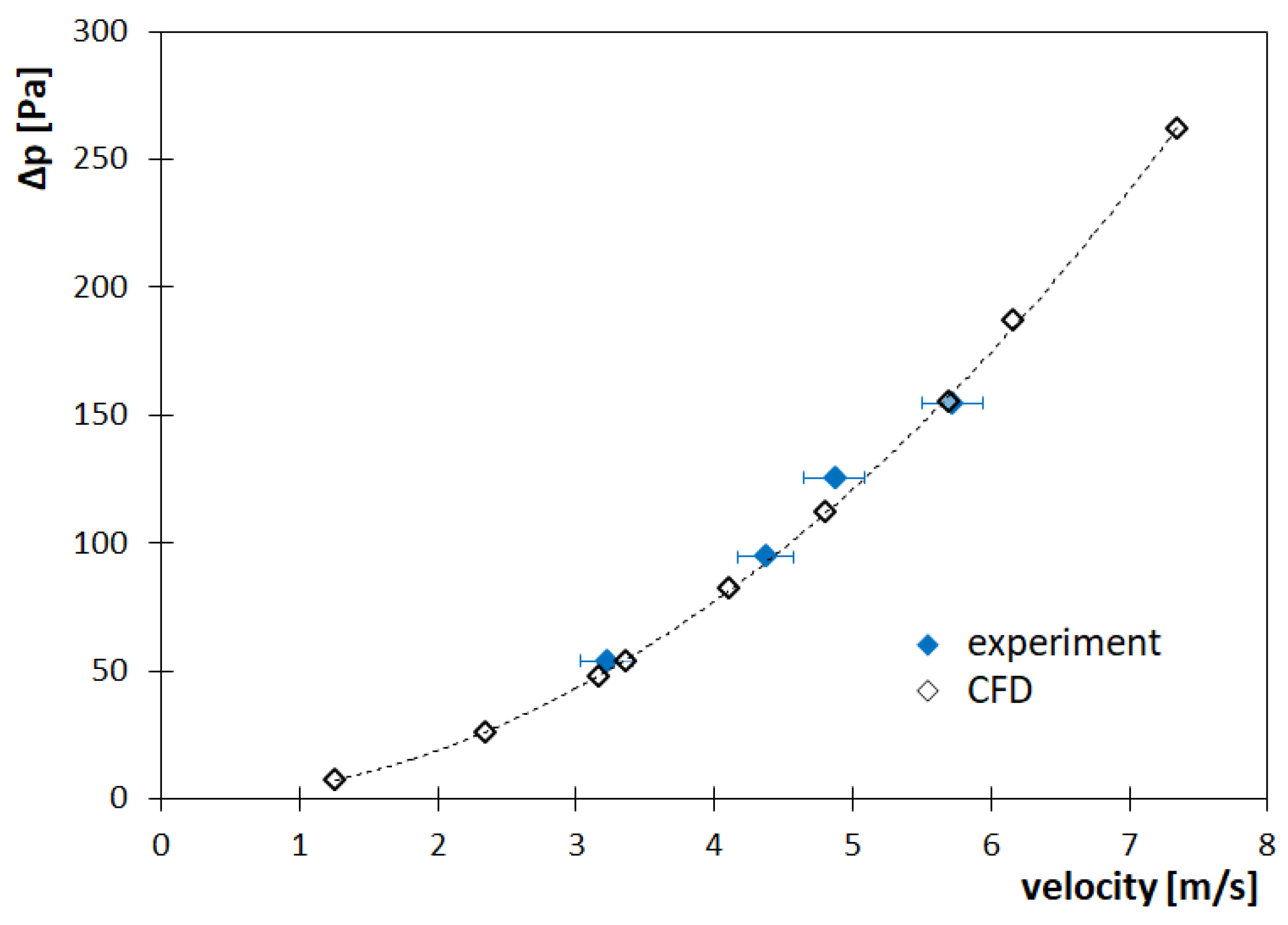
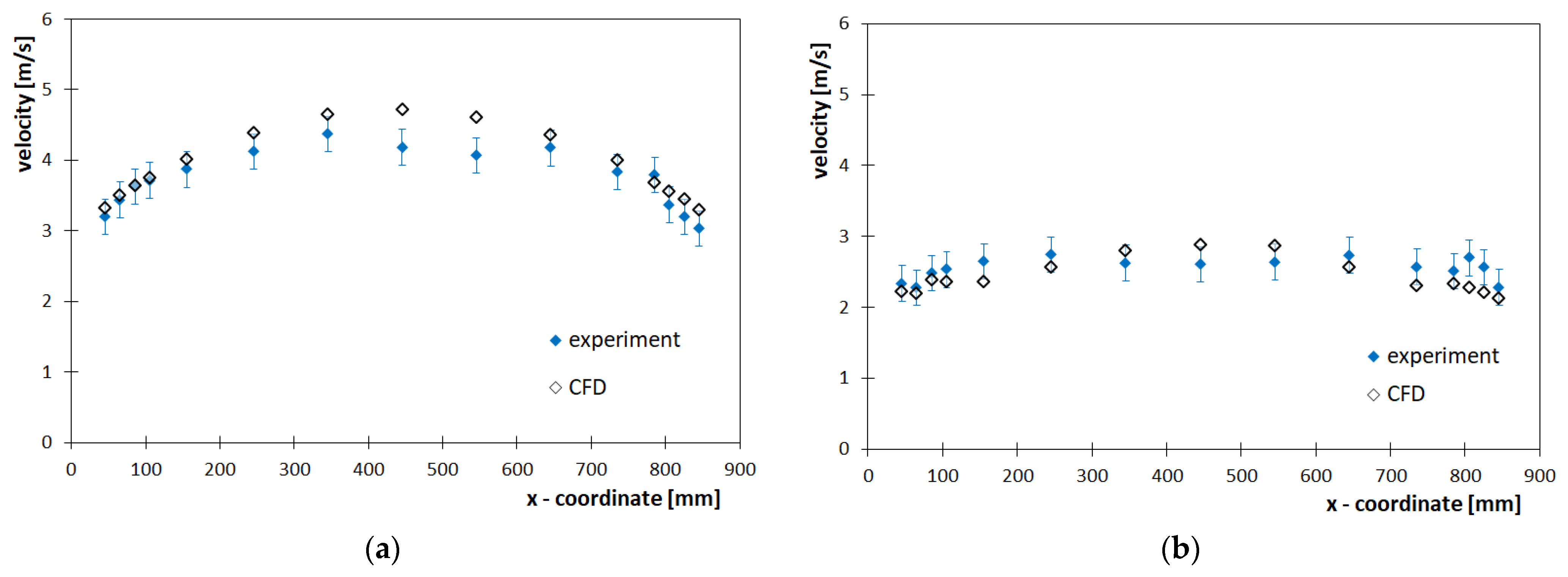
| 4 | comparison of numerical and experimental results | data statistics (Figure 5, Figure 6 and Figure 7) |
| 5 | numerical studies of the plate with different open area ratios | numerical results database: pressure drop, velocity distribution, coefficient C2 (Table 4 and Table 5) |
| 6 | development of correlation for pressure drop for all plates | correlation for pressure drop (Equation (11)) |
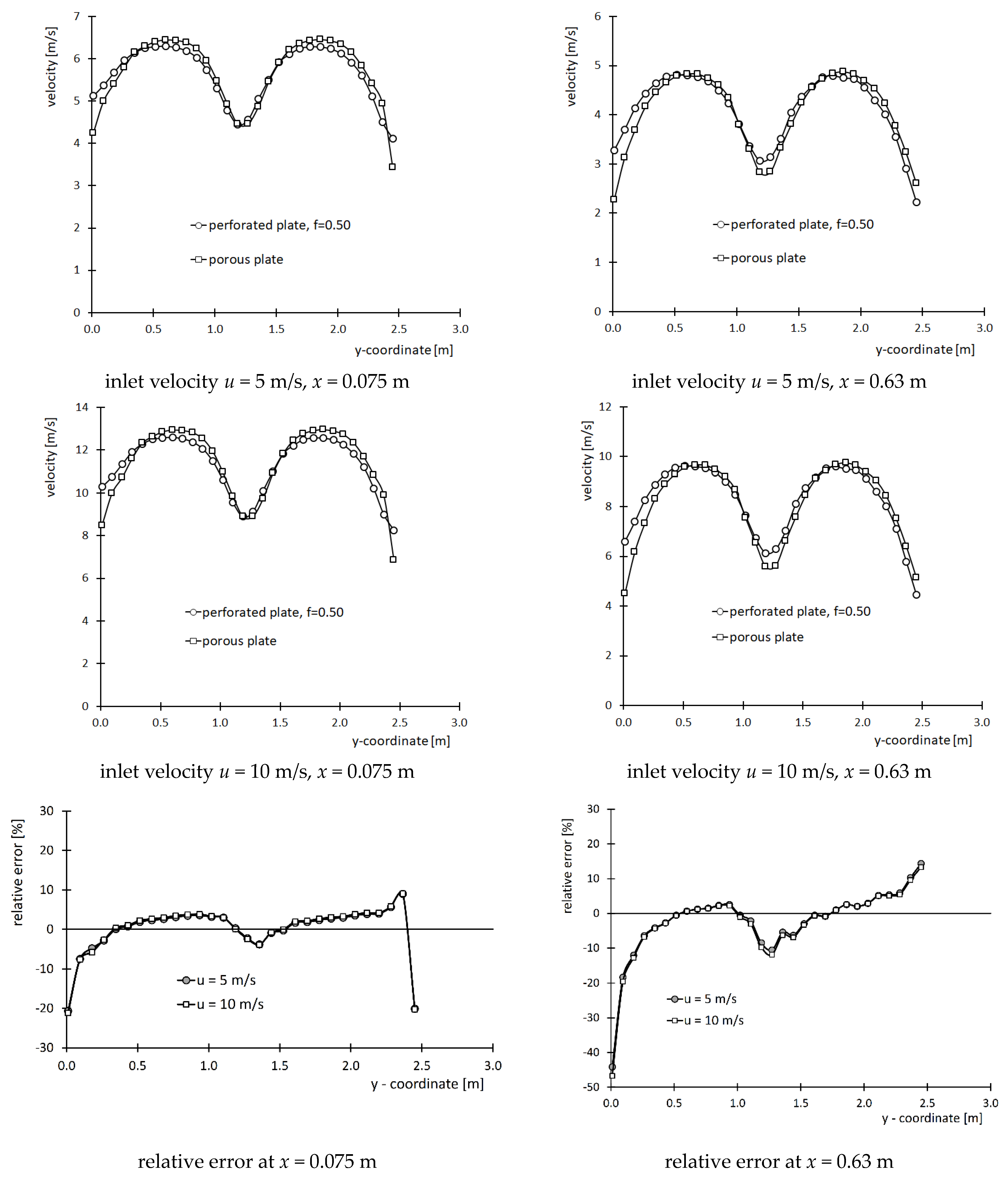
| 7 | numerical studies of the porous plate using developed correlation | data statistics (Figure 8 and Figure 9) |
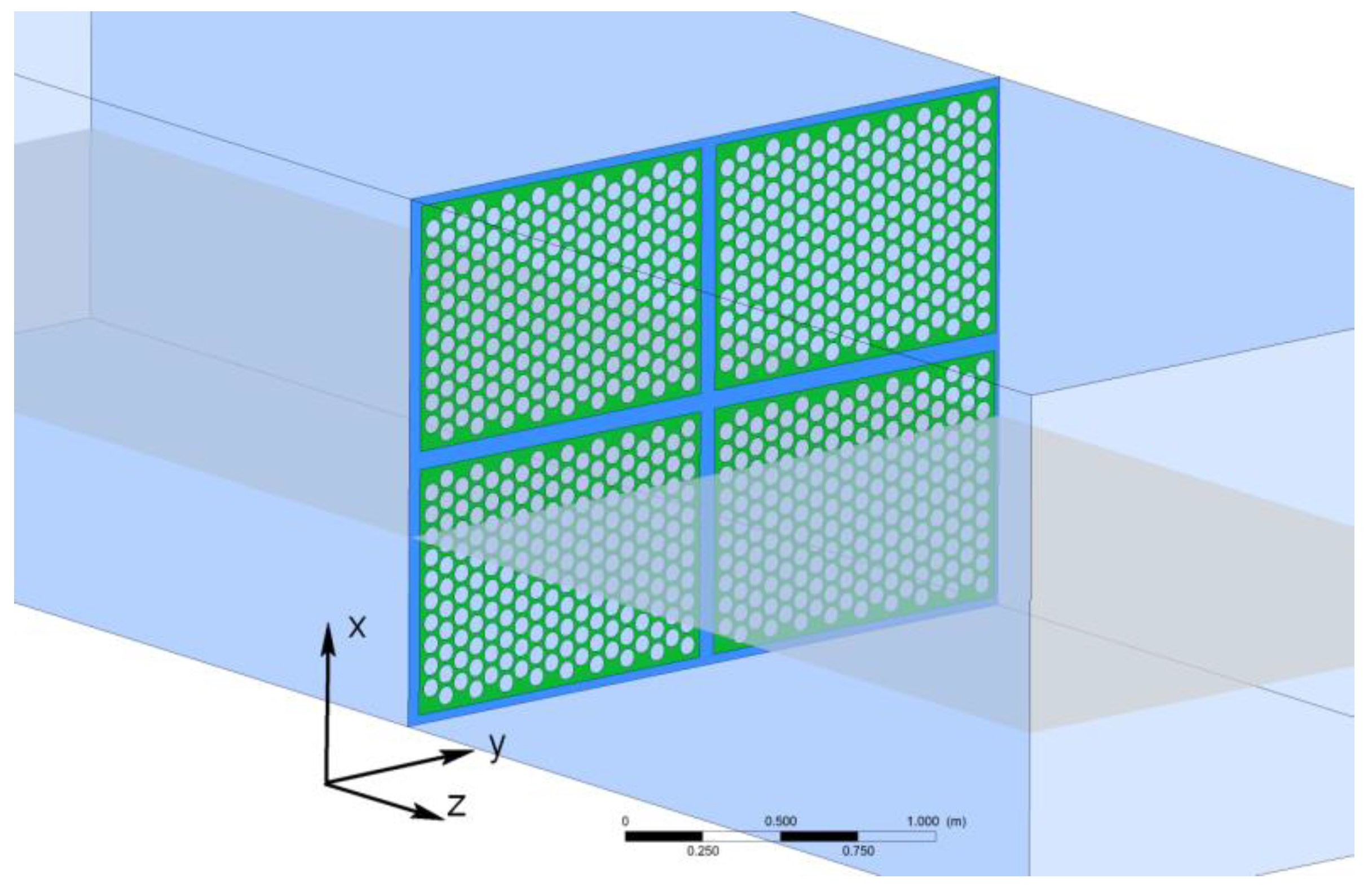
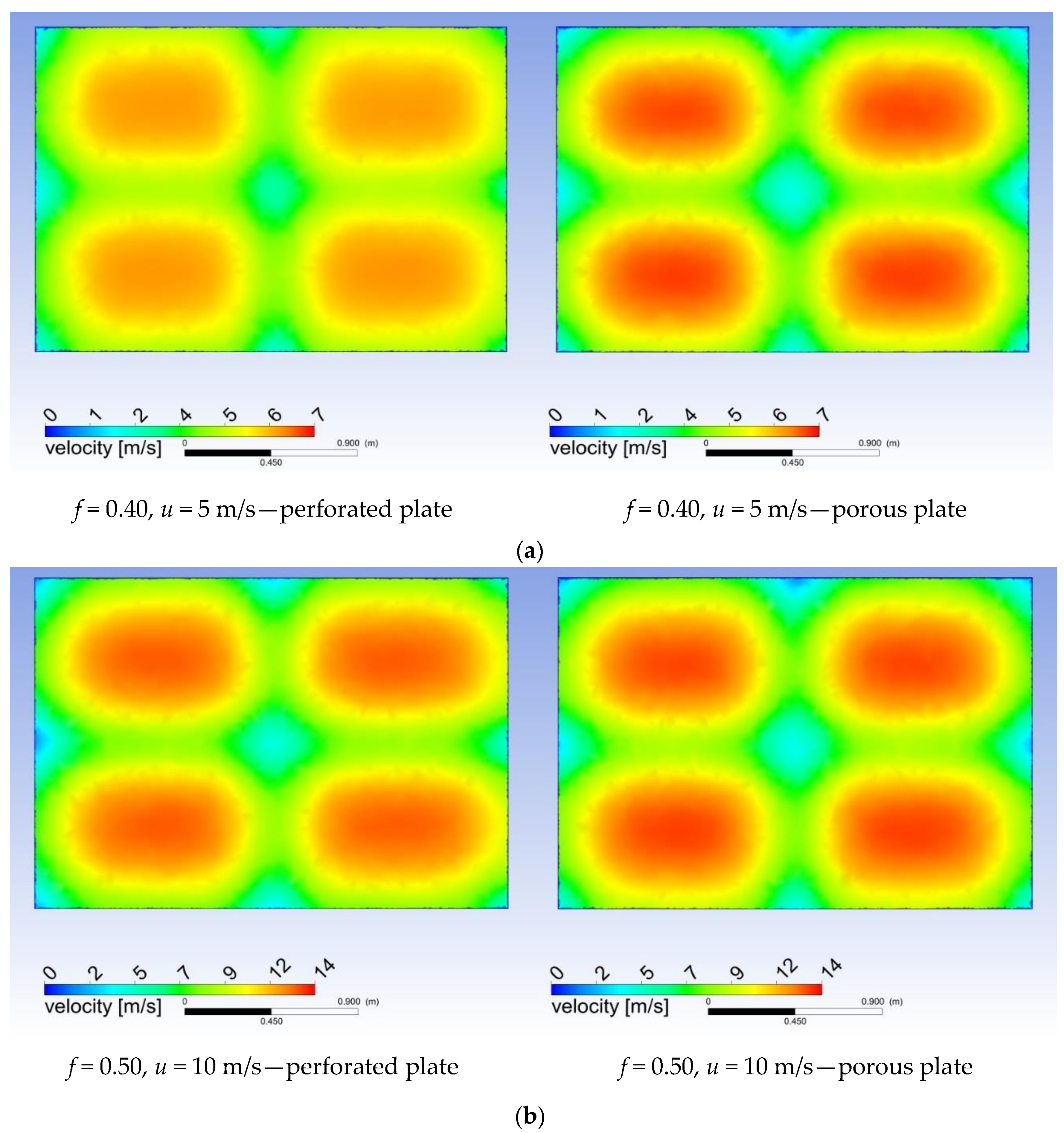
| 8 | numerical studies of the perforated panel with different open area ratios including structural elements | numerical results database: pressure drop, velocity distribution (Table 6, Figure 12, Figure 13, Figure 14 and Figure 15) |
| 9 | numerical studies of the porous panel including structural elements | numerical results data base: pressure drop, velocity distribution (Table 6, Figure 12, Figure 13, Figure 14 and Figure 15) |
| 10 | validation of results: perforated panel vs. porous panel | data statistics, general conclusions |
| Mesh No. | Number of Cells | Pressure Drop, Δp [Pa] | |
|---|---|---|---|
| 1 | 280,640 | 138.29 | - |
| 2 | 518,090 | 141.86 | 2.52 |
| 3 | 724,520 | 143.61 | 1.22 |
| 4 | 1,438,303 | 144.75 | 0.788 |
| 5 | 2,685,433 | 145.02 | 0.186 |
| 6 | 4,103,286 | 145.18 | 0.110 |
| Measurement No. | ΔpEXP [Pa] | ΔpCFD [Pa] | RE [%] | uEXP [m/s] | uCFD [m/s] | RE [%] |
|---|---|---|---|---|---|---|
| 1 | 53.93 ± 1.28 | 53.89 | −0.07 | 3.22 ± 0.19 | 3.34 | 3.73 |
| 2 | 94.72 ± 0.75 | 95.26 | 0.57 | 4.37 ± 0.20 | 4.44 | 1.60 |
| 3 | 125.59 ± 1.84 | 126.70 | 0.88 | 4.87 ± 0.22 | 5.12 | 5.13 |
| 4 | 154.70 ± 2.74 | 156.06 | 0.88 | 5.72 ± 0.22 | 5.69 | −0.53 |
| Velocity [m/s] | |||||
|---|---|---|---|---|---|
| f | 1 | 3 | 5 | 7 | 9 |
| - | Pressure Drop [Pa] | ||||
| 0.30 | 2515 | 22,648 | 62,926 | 123,351 | 203,923 |
| 0.35 | 1527 | 13,718 | 38,092 | 74,648 | 123,385 |
| 0.40 | 963 | 8634 | 23,963 | 46,948 | 77,589 |
| 0.44 | 681 | 6087 | 16,886 | 33,076 | 54,654 |
| 0.50 | 358 | 3140 | 8675 | 16,955 | 27,978 |
| 0.55 | 263 | 2289 | 6305 | 12,306 | 20,289 |
| 0.60 | 225 | 2009 | 5570 | 10,908 | 18,022 |
| 0.69 | 134 | 1188 | 3291 | 6442 | 10,640 |
| Open Area Ratio | Coefficient C2 |
|---|---|
| 0.30 | 4368.62 |
| 0.35 | 2592.16 |
| 0.40 | 1649.31 |
| 0.44 | 1194.39 |
| 0.50 | 774.76 |
| 0.55 | 561.06 |
| 0.60 | 417.88 |
| 0.69 | 247.96 |
| Perforated Plates Panel | Porous Plates Panel | RE | Perforated Plates Panel | Porous Plates Panel | RE | |
|---|---|---|---|---|---|---|
| u [m/s] | Δp [Pa] | Δp [Pa] | [%] | u [m/s] | u [m/s] | [%] |
| f = 0.40 | f = 0.40 | |||||
| 5 | 147.67 | 144.75 | 2.02 | 4.970 | 4.962 | 0.16 |
| 10 | 590.72 | 573.48 | 3.01 | 9.940 | 9.925 | 0.15 |
| f = 0.50 | f = 0.50 | |||||
| 5 | 76.70 | 76.13 | 0.74 | 4.978 | 4.962 | 0.32 |
| 10 | 306.82 | 298.48 | 2.79 | 9.956 | 9.924 | 0.32 |
| f = 0.55 | f = 0.55 | |||||
| 5 | 57.81 | 56.91 | 1.58 | 4.959 | 4.962 | 0.06 |
| 10 | 231.22 | 221.47 | 4.40 | 9.919 | 9.924 | 0.05 |
| f = 0.60 | f = 0.60 | |||||
| 5 | 46.59 | 48.13 | 3.20 | 4.999 | 4.998 | 0.02 |
| 10 | 186.17 | 186.23 | 0.30 | 9.999 | 9.997 | 0.02 |
Publisher’s Note: MDPI stays neutral with regard to jurisdictional claims in published maps and institutional affiliations. |
© 2021 by the authors. Licensee MDPI, Basel, Switzerland. This article is an open access article distributed under the terms and conditions of the Creative Commons Attribution (CC BY) license (https://creativecommons.org/licenses/by/4.0/).
Share and Cite
Śmierciew, K.; Butrymowicz, D.; Karwacki, J.; Gagan, J. Numerical Prediction of Homogeneity of Gas Flow through Perforated Plates. Processes 2021, 9, 1770. https://doi.org/10.3390/pr9101770
Śmierciew K, Butrymowicz D, Karwacki J, Gagan J. Numerical Prediction of Homogeneity of Gas Flow through Perforated Plates. Processes. 2021; 9(10):1770. https://doi.org/10.3390/pr9101770
Chicago/Turabian StyleŚmierciew, Kamil, Dariusz Butrymowicz, Jarosław Karwacki, and Jerzy Gagan. 2021. "Numerical Prediction of Homogeneity of Gas Flow through Perforated Plates" Processes 9, no. 10: 1770. https://doi.org/10.3390/pr9101770
APA StyleŚmierciew, K., Butrymowicz, D., Karwacki, J., & Gagan, J. (2021). Numerical Prediction of Homogeneity of Gas Flow through Perforated Plates. Processes, 9(10), 1770. https://doi.org/10.3390/pr9101770