Diagnostics of a Domestic Hot Water Storage Tank under Operating Conditions

Abstract

This paper presents a new method for the diagnostics of a hot water storage tank under operating conditions. Depending on the operating point of the tank, the method enables determination of thermal conductivity coefficients of the coil heat exchanger, which allows us to determine the intensity of heat transfer between the transfer medium and water in the tank as well as of tank walls, which consequently enables determination of heat losses to the environment. Furthermore, the dynamic properties of the tank may also be determined by applying this method. The advantage of this method is possibility of analyzing changes in the material constants of the coil heat exchanger, tank walls, and dynamic properties of the tank as a function of mass flow of the medium supplying the coil heat exchanger. The possibility of determining coefficients of thermal conductivity as well as the inertia of tank and exchanger, based on temperature measurements acquired in operating conditions is a novelty in this paper. Knowing the variability of material constants and of dynamic properties of the tank as a function of medium flow rate allows multicriteria optimization to be performed which, with a conventional design of the tank, results in a reduction of up to 10% in the time taken to prepare domestic hot water.

1. Introduction

One of the most important design parameters of a domestic hot water storage tank (DHWST) is the heat exchanger, which is installed inside the tank. The design parameters of the heat exchanger, such as heat transfer surface area in relation to the tank’s volume and the material from which it is made, determine its power and heat transfer rate, which affects the time it takes to prepare hot water. The time for preparing hot water is also determined by the operating parameters, among others, temperature and volumetric flow of the heat transfer medium [1,2,3]. In practice, the hot water preparation time in the tank is expected to be as short as possible, which, irrespective of the number of consumer points, ensures that the system is comfortable to operate. One of the methods to reduce the time for preparation of hot water is to introduce stratification in the storage tank, which determines its size and shape and the shape and structural materials of the heat exchanger inside the tank [4,5]. Furthermore, improved stratification can be achieved by insulating the inner wall surface with an insulating material or other low thermal conductivity material compatible with the stored liquid [6,7,8]. At present, a frequent design solution for stratification of water in the storage tank is a tank with a built-in thermosiphon heat exchanger [9,10]. Due to the special design in the form of a thermosiphon inside the heat exchanger, hot water preparation time is reduced by up to 65% compared to a storage tank fitted with a conventional heat exchanger. However, this solution is significantly more expensive than a storage tank with a conventional heat exchanger, therefore optimization of the design of the coil heat exchanger installed in a hot water storage tank still poses a current and very important research problem, as well as a challenge for engineers [11,12,13]. In practice, domestic hot water storage tanks are varied in terms of the heat exchanger geometry and material in order to improve the heat exchange intensity and consequently reduce the time taken to prepare domestic hot water. For this reason, domestic hot water storage tanks are designed to be operated with a specific heat source, which determines the design, the developed heat transfer surface area of the exchanger and the materials used for its fabrication. It is assumed that in the case of condensing gas or oil boilers, manufacturers recommend the use of storage tanks with a built-in heat exchanger with the developed surface of 1 m² per 1 kW of the heating capacity of the device. In the case of a solar heating system, the developed heat transfer surface of the heat exchanger should be larger. It is assumed that per 1 kW of solar system heating capacity, the developed heat transfer surface should be 0.6 m². In the case of a compressor heat pump, the developed heat exchange surface area of the heat exchanger should be even greater at 0.25 m² per 1 kW of heating capacity of the device [14]. Today, computational fluid dynamics modeling (CFD) is more and more often being used to design and analyze the thermal states of domestic hot water storage tanks. CFD analysis makes it possible to assess the impact of storage tank design parameters such as heat exchanger configuration [12], heat exchanger and tank wall material constants, operating conditions, and tank operating point [15,16] on the storage tank thermal performance. In practice, due to the variability of the operating point of the storage tank under operating conditions, at the design stage, even using CFD analyses, it is very difficult to predict how and within what limits the values of the material constants will change. The authors’ operating experience shows that in practice, storage tanks are often improperly selected for the heat source they are operated with, which translates into a significant increase in hot water preparation time. This is particularly evident in systems where compressor heat pumps are used as heat sources. Therefore, it becomes important to determine the material constants of the key structural components, including the heat exchanger, under the operating conditions and their dynamic properties, which will make it possible to analyze the impact of changing the operating point of the heat exchanger on its operating parameters and allow multicriteria optimization to be carried out in order to improve the performance of the tank. In this regard, the method for diagnostics of hot water storage tank under operating conditions developed by the authors is a novel approach, enabling improvement of thermal properties of the tank.

2. Methodology

The most important operating parameters of the hot water tank are inertia of the tank and heat exchange surface of the exchanger. The intensity of the heat exchange process results from heat exchange surface and the material from which the exchanger is made, which is characterized by the heat conductivity coefficient expressed in [W/m²K]. The value of the heat conductivity coefficient is strongly related to operating parameters of the tank, including water temperature within the tank, temperature of the medium supplying the exchanger, and the volumetric flow. These parameters characterize the so-called operating point of the tank, which is dependent on them. The values of these parameters vary under operating conditions, therefore it is very important to determine the heat conductivity coefficient of the exchanger at a given operating point as a function of the volumetric flow of the medium supplying this exchanger. For this reason, the parameters mentioned above were selected for analysis, as described below.

The proposed diagnostics method is based on the comparison of two models: an analytical model, in the form of a system of differential equations, developed on the basis of an energy balance linking the characteristic parameters of the storage tank (thermal conductivity coefficients, tank volume, etc.) with an operational model, in the form of differential equations, developed on the basis of operational data using parametric identification. A prerequisite for the reliability of this method is the same order of analytical and parametric model. The System Identification library of the Matlab package was used to develop an operational model based on the operational data, therefore, the paper will explain the part of the methodology concerning the analytical model.

2.1. The Operational Analytical Model of a Domestic Hot Water Storage Tank Based on Energy Balance

The operational model of the storage tank based on energy balance was developed assuming that the water temperature in the tank is distributed uniformly over the entire height of the coil heat exchanger. The model therefore does not take into account possible stratification that may occur in the storage tank. However, in modern heating systems, due to the requirements of the users, internal circulation is ensured to compensate for stratification in the storage tank.

Assuming that the modeled hot water storage tank is a load for a solar collector array and is isolated from the solar segment by a coil heat exchanger placed inside the storage tank, the amount of heat supplied by the collector array to the tank can be determined from Equation (1).

$$P=\dot{m}{\mathrm{c}}_{\mathrm{p}}\ast \left(T_{in}-T_{out}\right)$$

(1)

Assuming that the distribution of water temperature in the storage tank over the height of the heat exchanger is uniform, the amount of heat received by the water in the storage tank can be calculated from Equation (2).

$$P_{odd}=U_{LW}\left(\frac{T_{in}+T_{out}}{2}-T_{zas}\right)$$

(2)

In a steady state, the amount of heat supplied by the heat exchanger is equal to the amount of heat received by the water in the tank. Equation (3) is, therefore, true.

$$P=P_{odd}$$

(3)

Therefore, by substituting Equations (1) and (2) into Equation (3), it is possible to determine the outlet temperature of the medium from the heat exchanger according to Equation (4).

$$T_{out}=\frac{2\dot{m}{\mathrm{c}}_{\mathrm{p}}{T}_{in}+U_{LW}\ast \left(2T_{zas}-T_{in}\right)}{2{\dot{m}\mathrm{c}}_{\mathrm{p}}+U_{LW}}$$

(4)

Assuming that the recorded curves of the inlet and outlet temperatures of the medium are dependent on the temperature of the water in the storage tank, Equation (4) can be simplified to the form 5.

$$T_{out}=\frac{2\dot{m}{\mathrm{c}}_{\mathrm{p}}{T}_{in}-U_{LW}\ast T_{in}}{2{\dot{m}\mathrm{c}}_{\mathrm{p}}+U_{LW}}$$

(5)

According to Equation (5), the variation of the outlet temperature of the medium from the heat exchanger depends on the value of the U_LW coefficient, the inlet temperature, the flow rate, and the specific heat of the medium in the system.

The temperature rise in a domestic hot water storage tank depends not only on the thermal capacity of the storage tank but also on the dynamic properties of the heat exchanger inside the storage tank. The dynamic properties of the heat exchanger can be determined from the differential equation.

$${\left(mc\right)}_{eW}\frac{d{T}_{out}\left(t\right)}{dt}=\dot{m}{\mathrm{c}}_{\mathrm{p}}\left(T_{in}\left(t\right)-T_{out}\left(t\right)\right)-U_{LW}\left(\frac{T_{in}\left(t\right)+T_{out}\left(t\right)}{2}-T_{zas}\left(t\right)\right)$$

(6)

By transforming Equation (6) into the form (7) and completing the Laplace transform, Equation (8) is obtained, which enables determination of the transition state of the outlet temperature of the medium from the coil.

$$\frac{2{\left(mc\right)}_{eW}}{U_{LW}+2\dot{m}{\mathrm{c}}_{\mathrm{p}}}\frac{d{T}_{out}\left(t\right)}{dt}+T_{out}\left(t\right)=\left(\frac{2\dot{m}{\mathrm{c}}_{\mathrm{p}}-U_{LW}}{U_{LW}+2\dot{m}{\mathrm{c}}_{\mathrm{p}}}\right)T_{in}\left(t\right)+\left(\frac{2U_{LW}}{U_{LW}+2\dot{m}{\mathrm{c}}_{\mathrm{p}}}\right)T_{zas}\left(t\right)$$

(7)

$$T_{out }\left(s\right)=\underset{\underset{\mathit{Main} \mathit{path}}{⏟}}{\frac{\left(\frac{2\dot{m}{\mathrm{c}}_{\mathrm{p}}-U_{LW}}{U_{LW}+2\dot{m}{\mathrm{c}}_{\mathrm{p}}}\right)}{\frac{2{\left(mc\right)}_{ew}}{U_{LW}+2\dot{m}{\mathrm{c}}_{\mathrm{p}}}s+1}{T}_{in}\left(s\right)}+\underset{\underset{\mathit{Disturbance} \mathit{path}}{⏟}}{\frac{\left(\frac{2U_{LW}}{U_{LW}+2\dot{m}{\mathrm{c}}_{\mathrm{p}}}\right)}{\frac{2{\left(mc\right)}_{eW}}{U_{LW}+2\dot{m}{\mathrm{c}}_{\mathrm{p}}}s+1}{T}_{zas}\left(s\right)}$$

(8)

The model of the coil heat exchanger developed on the basis of the energy balance consists of two paths: the main path related to the medium inlet temperature, described in Equation (9) by the transfer function G₁(s), and the disturbance path related to the storage tank temperature, described in Equation (10) by the transfer function G₂(s). The operational model of the heat exchanger can be represented by a block diagram (Figure 1).

$$G_1\left(s\right)=\frac{\left(\frac{2\dot{m}{\mathrm{c}}_{\mathrm{p}}-U_{LW}}{U_{LW}+2\dot{m}{\mathrm{c}}_{\mathrm{p}}}\right)}{\frac{2{\left(mc\right)}_{ew}}{U_{LW}+2\dot{m}{\mathrm{c}}_{\mathrm{p}}}s+1}$$

(9)

$$G_2\left(s\right)=\frac{\left(\frac{2U_{LW}}{U_{LW}+2\dot{m}{\mathrm{c}}_{\mathrm{p}}}\right)}{\frac{2{\left(mc\right)}_{eW}}{U_{LW}+2\dot{m}{\mathrm{c}}_{\mathrm{p}}}s+1}$$

(10)

The individual constituent paths of the model are described with the transfer function, appropriate for a first-order inertial object. The gain factors of the individual paths can be determined from Equations (11) and (12), and the equivalent time constant, which is identical for both paths of the model, can be determined from Equation (13).

$${kp}_1=\left(\frac{2\dot{m}{\mathrm{c}}_{\mathrm{p}}-U_{LW}}{U_{LW}+2\dot{m}{\mathrm{c}}_{\mathrm{p}}}\right)$$

(11)

$$k{p}_2=\left(\frac{2U_{LW}}{U_{LW}+2\dot{m}{\mathrm{c}}_{\mathrm{p}}}\right)$$

(12)

$$T_{zW}=\frac{2{\left(mc\right)}_{eW}}{U_{LW}+2\dot{m}{\mathrm{c}}_{\mathrm{p}}}$$

(13)

Equations (11) and (12) show that the gain factors of both model paths depend on the flow and specific heat of the medium and the U_LW coefficient. The equivalent time constant is related to the effective heat capacity of the heat exchanger and the flow rate and specific heat of the medium.

Assuming that there is no stratification in the storage tank over the height of the heat exchanger and that the amount of heat transferred by the coil is equal to the amount of heat received by the water in the storage tank, the energy balance of the tank can be described using Equation (14).

$$\frac{2U_{LW}\dot{m}{\mathrm{c}}_{\mathrm{p}}\left(T_{in}-T_{zas}\right)}{2\dot{m}{\mathrm{c}}_{\mathrm{p}}+U_{LW}}-U_{LZ}\left(T_{zas}-T_{amb}\right)=0$$

(14)

The temperature of the water in the storage tank can be calculated by transforming Equation (14) into the form:

$$T_{zas}=\frac{2U_{LW}\dot{m}{\mathrm{c}}_{\mathrm{p}}{T}_{in}+U_{LZ}{T}_{amb}\left(2\dot{m}{\mathrm{c}}_{\mathrm{p}}+U_{LW}\right)}{2\dot{m}{\mathrm{c}}_{\mathrm{p}} \left(U_{LW}+U_{LZ}\right)+U_{LW}{U}_{LZ}}$$

(15)

According to Equation (15), the water temperature rise in the storage tank depends on the inlet temperature of the medium to the coil and the specific heat and flow rate of the medium.

The water temperature rise in the storage tank depends on the amount of heat transferred through the heat exchanger and the heat losses through the tank walls. Knowing the amount of heat transferred by the heat exchanger into the storage tank and the heat losses from the tank to the environment, the temperature rise in the tank can be estimated using the Equation:

$${\left(mc\right)}_{ezas}\frac{d{T}_{zas}}{dt}=\frac{2U_{LW}\dot{m}{\mathrm{c}}_{\mathrm{p}}\left(T_{in}\left(t\right)-T_{zas\left(t\right)}\right)}{2\dot{m}{\mathrm{c}}_{\mathrm{p}}+U_{LW}}-U_{LZ}\left(T_{zas}\left(t\right)-T_{amb}\left(t\right)\right)$$

(16)

By transforming Equation (16) and rearranging it, we can obtain the Equation

$$\frac{\left(2\dot{m}{c}_p+U_{LW}\right){\left(mc\right)}_{ezas}}{2\dot{m}{c}_p \left(U_{LW}+U_{LZ}\right)+U_{LW}{U}_{LZ}}\frac{d{T}_{zas}\left(t\right)}{dt}+T_{zas}\left(t\right)=\frac{2U_{LW}\dot{m}{c}_p{T}_{in}\left(t\right)}{2\dot{m}{c}_p \left(U_{LW}+U_{LZ}\right)+U_{LW}{U}_{LZ}}+\frac{U_{LZ}{T}_{amb}\left(t\right)\left(2\dot{m}{c}_p+U_{LW}\right)}{2\dot{m}{c}_p \left(U_{LW}+U_{LZ}\right)+U_{LW}{U}_{LZ}}$$

(17)

By transforming Equation (17) using the Laplace transform into the domain of a complex variable, the operational model of the storage tank (18) is obtained, which makes it possible to determine the dynamic properties in the time domain.

$${\mathit{T}}_{\mathit{z}\mathit{a}\mathit{s}}\left(\mathrm{s}\right)=\underset{\underset{Main path}{⏟}}{\frac{\frac{2U_{LW}{\dot{m}\mathrm{c}}_{\mathrm{p}}}{2{\dot{m}\mathrm{c}}_{\mathrm{p}}\left(U_{LW}+U_{LZ}\right)+U_{LW}{U}_{LZ}}}{\frac{\left(2{\dot{m}\mathrm{c}}_{\mathrm{p}}+U_{LW}\right){\left(mc\right)}_{eZ}}{2{\dot{m}\mathrm{c}}_{\mathrm{p}} \left(U_{LW}+U_{LZ}\right)+U_{LW}{U}_{LZ}}s+1}{T}_{in}\left(s\right)}+\underset{\underset{Disturbance path}{⏟}}{\frac{\frac{U_{LZ}\left(2{\dot{m}\mathrm{c}}_{\mathrm{p}}+U_{LW}\right)}{2{\dot{m}\mathrm{c}}_{\mathrm{p}} \left(U_{LW}+U_{LZ}\right)+U_{LW}{U}_{LZ}}}{\frac{\left(2{\dot{m}\mathrm{c}}_{\mathrm{p}}+U_{LW}\right){\left(mc\right)}_{eZ}}{2{\dot{m}\mathrm{c}}_{\mathrm{p}} \left(U_{LW}+U_{LZ}\right)+U_{LW}{U}_{LZ}}s+1}{T}_{amb}\left(s\right)}$$

(18)

Equation (18) shows that the storage tank model developed on the basis of the energy balance consists of two paths: the main path described with Equation (19) by the transfer function G₁(s), related to the medium inlet temperature T_in to the coil, and the disturbance path described with Equation (20) by the transfer function G₂(s) and related to the ambient temperature T_amb. The operational model of the storage tank can be represented by a block diagram (Figure 2).

$$G_1\left(s\right)=\frac{\frac{2U_{LW}\dot{m}{\mathrm{c}}_{\mathrm{p}}}{2\dot{m}{\mathrm{c}}_{\mathrm{p}}\left(U_{LW}+U_{LZ}\right)+U_{LW}{U}_{LZ}}}{\frac{\left(2\dot{m}{\mathrm{c}}_{\mathrm{p}}+U_{LW}\right){\left(mc\right)}_{eZ}}{2\dot{m}{\mathrm{c}}_{\mathrm{p}} \left(U_{LW}+U_{LZ}\right)+U_{LW}{U}_{LZ}}s+1}$$

(19)

$$G_2\left(s\right)=\frac{\frac{U_{LZ}\left(2\dot{m}{\mathrm{c}}_{\mathrm{p}}+U_{LW}\right)}{2\dot{m}{\mathrm{c}}_{\mathrm{p}} \left(U_{LW}+U_{LZ}\right)+U_{LW}{U}_{LZ}}}{\frac{\left(2\dot{m}{\mathrm{c}}_{\mathrm{p}}+U_{LW}\right){\left(mc\right)}_{eZ}}{2\dot{m}{\mathrm{c}}_{\mathrm{p}} \left(U_{LW}+U_{LZ}\right)+U_{LW}{U}_{LZ}}s+1}$$

(20)

The transfer functions of both paths are appropriate for first-order inertial objects. The transfer functions describing the dynamic properties of the individual paths make it possible to determine the gain factors and the equivalent time constants. The main path gain factor can be determined from Equation (21), while the disturbance path gain factor can be determined from Equation (22). The equivalent time constant is defined by Equation (23).

$$k{p}_1=\frac{2U_{LW}\dot{m}{\mathrm{c}}_{\mathrm{p}}}{2\dot{m}{\mathrm{c}}_{\mathrm{p}}\left(U_{LW}+U_{LZ}\right)+U_{LW}{U}_{LZ}}$$

(21)

$$k{p}_2=\frac{U_{LZ}\left(2\dot{m}{\mathrm{c}}_{\mathrm{p}}+U_{LW}\right)}{2\dot{m}{\mathrm{c}}_{\mathrm{p}} \left(U_{LW}+U_{LZ}\right)+U_{LW}{U}_{LZ}}$$

(22)

$$T_{zzas}\frac{\left(2\dot{m}{\mathrm{c}}_{\mathrm{p}}+U_{LW}\right){\left(mc\right)}_{eZ}}{2\dot{m}{\mathrm{c}}_{\mathrm{p}} \left(U_{LW}+U_{LZ}\right)+U_{LW}{U}_{LZ}}$$

(23)

The holistic model of the DHW storage tank can be represented with the following block diagram (Figure 3).

According to the diagram in Figure 3, the DHW storage tank consists of two interdependent objects: the coil heat exchanger and the water tank.

The inlet temperature of the medium to the heat exchanger and the ambient temperature were taken as input signals, and the outlet temperature of the medium from the exchanger was taken as the output signal. The water temperature in the heat exchanger is the variable that links the two parts of the storage tank model. According to the diagram of the storage tank shown in Figure 3, the parametric identification process would need to develop two independent models of the individual components of the storage tank, linked together by the water temperature in the storage tank. Consequently, in terms of its structure, the model would become complex. Assuming that the recorded curves of the inlet and outlet temperatures of the medium from the exchanger and the water temperature in the storage tank, as a function of time, are interdependent on each other and on the ambient temperature, the disturbance path can be neglected in both parts of the storage tank model. The operational model of the DHW storage tank is then simplified to the form represented with the block diagram in Figure 4. The dynamic properties of the main path of the operational model are described by the transfer function (24) and of the disturbance path—by the transfer function (25), the gain factors and the equivalent time constants of which can be estimated using Equations (26)–(29).

$$T_{out }\left(s\right)=\frac{\left(\frac{2\dot{m}{\mathrm{c}}_{\mathrm{p}}-U_{LW}}{U_{LW}+2\dot{m}{\mathrm{c}}_{\mathrm{p}}}\right)}{\frac{2{\left(mc\right)}_{eW}}{U_{LW}+2\dot{m}{\mathrm{c}}_{\mathrm{p}}}s+1}{T}_{in}$$

(24)

$$T_{out }\left(s\right)=\frac{\left(\frac{2\dot{m}{\mathrm{c}}_{\mathrm{p}}-U_{LW}}{U_{LW}+2\dot{m}{\mathrm{c}}_{\mathrm{p}}}\right)}{\frac{2{\left(mc\right)}_{eW}}{U_{LW}+2\dot{m}{\mathrm{c}}_{\mathrm{p}}}s+1}{T}_{in}$$

(25)

$$k{p}_1=\left(\frac{2\dot{m}{\mathrm{c}}_{\mathrm{p}}-U_{LW}}{U_{LW}+2\dot{m}{\mathrm{c}}_{\mathrm{p}}}\right)$$

(26)

$$T_{zW}=\frac{2{\left(mc\right)}_{eW}}{U_{LW}+2\dot{m}{\mathrm{c}}_{\mathrm{p}}}$$

(27)

$$k{p}_2=\frac{2U_{LW}\dot{m}{\mathrm{c}}_{\mathrm{p}}}{2\dot{m}{\mathrm{c}}_{\mathrm{p}}\left(U_{LW}+U_{LZ}\right)+U_{LW}{U}_{LZ}}$$

(28)

$$T_{zzas}=\frac{\left(2\dot{m}{\mathrm{c}}_{\mathrm{p}}+U_{LW}\right){\left(mc\right)}_{eZ}}{2\dot{m}{\mathrm{c}}_{\mathrm{p}} \left(U_{LW}+U_{LZ}\right)+U_{LW}{U}_{LZ}}$$

(29)

The U_LW and U_LZ coefficients in the individual transfer functions of the paths of the model parts correspond to the heat loss coefficients. The U_LW coefficient corresponds to the heat losses of the coil heat exchanger and the U_LZ coefficient corresponds to the heat losses of the storage tank. The energy balance shows that the power supplied by the heat exchanger should be equal to the power transferred to the storage tank. Therefore, the gain factors of both paths of the operational model of the D_HW storage tank should be 1. The heat losses from the coil heat exchanger—U_LW should be calculated with Equation (26). The power losses of the tank—U_LZ should be calculated with Equation (28), and the thermal capacity of the tank with Equation (29). The heat transfer intensity of the heat exchanger to the storage tank, that is the exchanger thermal conductivity coefficient λ_W, should be calculated using Equation (30).

$$\lambda w=\frac{2\dot{m}{\mathrm{c}}_{\mathrm{p}}-\left(\left(1-k_{pw1}\right)\ast 2\dot{m}{\mathrm{c}}_{\mathrm{p}}\right)}{\left(1-k_{pw1}\right)+1}\left[\frac{W}{K}\right]$$

(30)

2.2. Storage Tank Model Based on Operational Data

The diagnostics of a storage tank is illustrated by the operating data recorded during the operation of the solar heating system (Figure 5). The system consisted of two flat solar collectors with a unit absorber area of 3 m². The collectors were thermally loaded with a 100 dm³ storage tank fitted with a coil heat exchanger with a volume of 2.3 m³ and a developed heat transfer surface area of 0.75 m² (Figure 6). The exchanger’s declared power, according to the manufacturer, is 14 kW at the flow rate of the heating medium of 2.5 m³/h and the temperature of the heating medium of 70 °C, the temperature of feeding water of 10 °C, and the temperature of domestic hot water of 45 °C. The medium flow rate was forced by a pump with stepless adjustment between 2 and 9 l/min, and it was measured using a flow meter generating a voltage signal corresponding to the flow rate, in the range of 0–10 V DC. The temperature was measured using four-wire PT1000 sensors, which made it possible to compensate for the resistance of the wires. The system control algorithm was implemented in a PLC which used a TCP/IP protocol for communication with a computer and the installed SCADA LBX software (ver. 2.60 LAB-EL, Reguły Poland, 2020). This solution made it possible to monitor the system and record the measurement data. The measurement data were sampled and recorded with a 1-s interval.

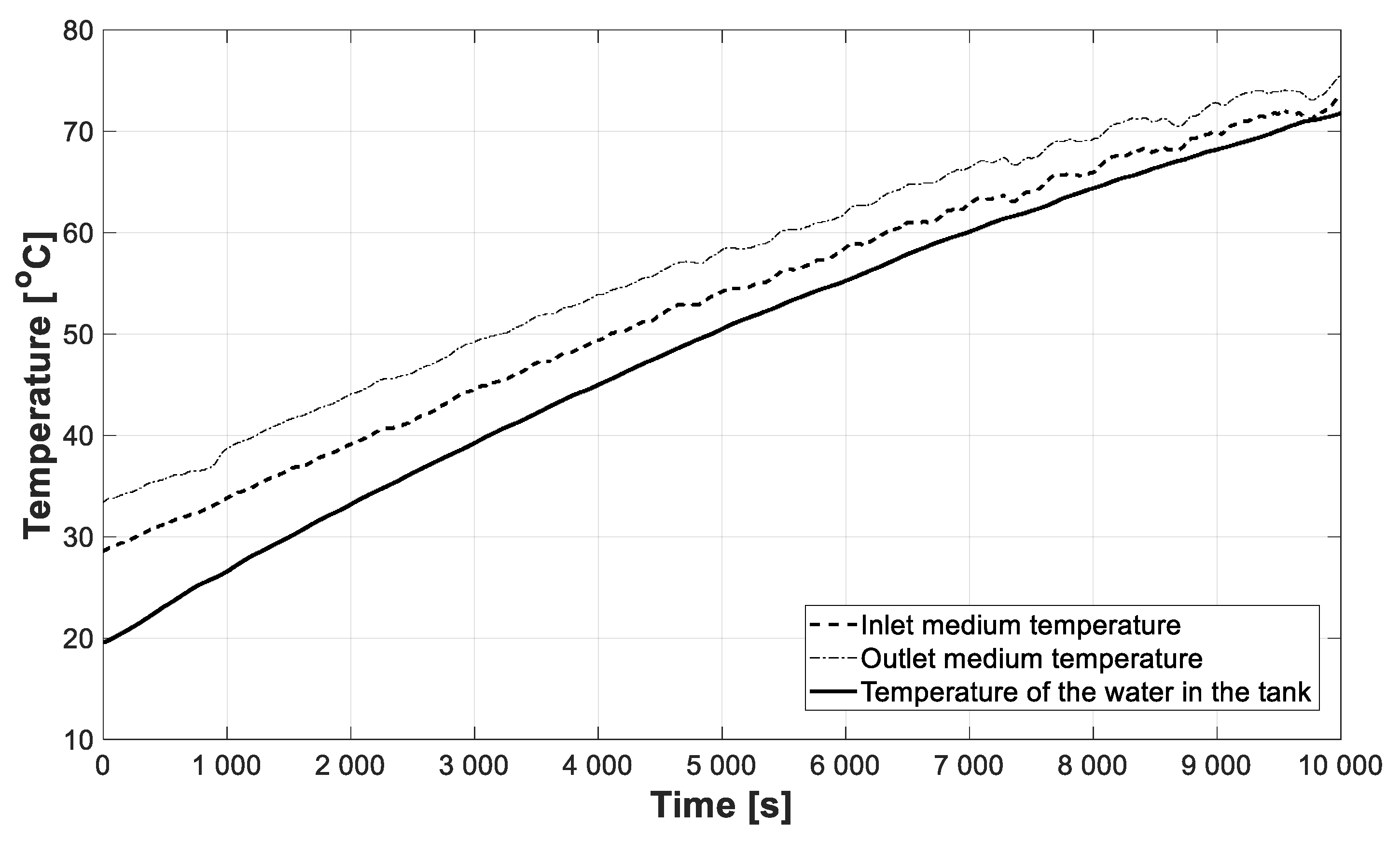
The operating data recorded at various operating points of the tank are to be used to diagnose the storage tank. In case of the solar heating system under consideration, the operating point will vary depending on prevailing sunlight conditions and flow of the working medium. The impact of working medium mass flow in solar installation on heat transfer coefficients as well as on thermal inertia of DHW storage tank and coil heat exchanger were analyzed on data recorded during 15 days of the installation operation. During each experiment, the mass flow of the working medium was constant, and the values of solar radiation intensity were high and stable over time. The instantaneous variability of the intensity of solar radiation during the experiment had a negligible impact on the dynamic properties of the reservoir (very high reservoir time constant) and the thermal conductivity coefficients. All experiments were performed for three mass flows of the working medium through the coil exchanger: the minimum one was 0.038 ± 0.02 [kg/s], the average one was 0.09 ± 0.02 [kg/s] and the maximum one was 0.13 ± 0.2 [kg/s]. Examples of operational data from one of these 15 days are presented in Figure 7. During the experiment that day, the medium flow through the heat exchanger was 0.132 [l/s]. On this basis, the proposed diagnostic method was discussed, but it should be emphasized that in the case of operational data recorded for the remaining 14 days, the procedure was identical.

In the identification process, the DHW storage tank was treated according to the analytical model as a single-input dual-output object (Figure 4). The inlet temperature of the medium to the coil, which is also the outlet temperature of the medium from the collector array, was taken as the input signal. The outlet temperature of the medium from the coil, which is also the inlet temperature of the medium to the collector array, and the temperature of the water in the storage tank were taken as the output signals. For temperature measurements, class A Pt1000 sensors were used for which the measurement uncertainty in the temperature range −30 °C–300 °C was (±0.15 + 0.002|t|). The operational model developed on the basis of such data enables the analysis of the dynamics of the coil heat exchanger—main path and the analysis of the dynamics of the water temperature in the storage tank—disturbance path.

In the parametric identification process, an operational model of the storage tank was developed based on the recorded operational data. The static and dynamic properties of the DHW storage tank were best represented by the ARX autoregressive model, described by a system of differential Equation (31), as estimated in the validation process (Figure 8). The determination coefficient of the model was 0.99.

$$\begin{array}{c}A\left(z\right)=1-0.998 z^{-1}\\ A_{2\left(z\right)}=-0.0003284 z^{-1}\\ B\left(z\right)=0.001627 z^{-1}\\ A\left(z\right)=1-0.9991 z^{-1}\\ A\_1\left(z\right)=-0.001188 z^{-1}\\ B\left(z\right)=-0.0001969 z^{-1}\end{array}$$

(31)

3. Analysis of Material Constants and Static and Dynamic Properties of the Storage Tank

In order to determine the dynamic properties of the coil and the storage tank, the operational model in the form of a system of differential Equation (31) was transformed using the Laplace transform to the form of transfer functions (32) and (34), and in order to compare it with the analytical model, on the basis of the step response curves of the main path and the disturbance path, it was approximated to the form of first-order transfer functions, which correspond to Formulas (33) and (35).

Figure 9 shows the step response of the main path of the operational model described by the transfer function (32).

$$G_1\left(\mathrm{s}\right)=\frac{0.001629\mathrm{s}+1.481\times {10}^{-6}}{{\mathrm{s}}^2+0.002919\mathrm{s}+1.479\times {10}^{-6}}$$

(32)

$$G_1\left(\mathrm{s}\right)=\frac{0.996}{717.33\mathrm{s}+1}$$

(33)

The main path is inertial, which is typical of thermal objects. The equivalent time constant read from the step response was 717.33 [s] and the static gain factor was kp₁ = 0.996. With the value of the gain factor, using Equation (30) it was possible to estimate the heat transfer rate in the heat exchanger, which, at a flow rate of 0.132 [l/s], was 943.1 [W/K]. The value of the heat loss coefficient calculated from Equation (26) was 2.33 [W/K]. Using Equation (27), the effective heat capacity of the coil heat exchanger can be determined. In the case under consideration, the heat capacity of the coil was 3.41 × 10⁵ [J/K].

A similar analysis can be made for the disturbance path of the storage tank model described by the transfer function (34).

$$G_2\left(\mathrm{s}\right)=\frac{-0.0001979\mathrm{s}+1.548\times {10}^{-6}}{{\mathrm{s}}^2+0.002919\mathrm{s}+1.479\times {10}^{-6}}$$

(34)

$$G_2\left(\mathrm{s}\right)=\frac{1.04}{2187.4\mathrm{s}+1}$$

(35)

Comparing the transfer functions of the two paths of the storage tank model, it should be noted that they have an identical characteristic equation. Discrepancies in the transient curves between the paths of the operational model of the storage tank will result from the position of the zeros (numerator radicals) relative to the poles (denominator radicals) of the transfer function in the plane of the complex variable. The position of the zeros relative to the poles depends on the mutual trajectories of the output signals relative to the input signal.

Figure 10 shows the step response of the disturbance path of the operational model of the DHW storage tank. On the basis of the transient curves, it should be concluded that the model’s disturbance path has a non-minimum-phase character. In the first phase, the output signal (storage tank temperature) trends in the opposite direction to the intended one, and then aperiodically reaches a steady state. It is also worth noting that the gain factor of the disturbance path was 1.04 which, despite the good insulation of the storage tank, indicates power loss. In the case under consideration, the power losses from the storage tank calculated from the relationship (21) were 19.4 [W/K].

The equivalent time constant determined from the step response was 2187.4 [s]. The time constant of the storage tank was three times longer than the equivalent time constant of the coil. The effective heat capacity of storage the tank at the height of the coil exchanger in the case under consideration was 9.92 × 10⁵ [J/K] as calculated from Equation (23).

4. Analysis of the Variation of Material Constants and Storage Tank Operating Parameters as a Function of the Medium Flow

The gain factors and the equivalent time constant, and thus the material constants of both paths of the operational model of the DHW storage tank, described by Equations (24) and (25), are strongly dependent on the performance of the circulator pump. Having operational data recorded with different circulator pump output, the impact of flow rate on the static and dynamic properties of the DHW storage tank can be estimated.

Figure 11 shows the impact of the circulator pump output $\dot{m}$ on the value of the gain factor kp1 of the main path of the DHW storage tank model. The figure shows that as the circulator pump output increases, the value of the gain factor also increases. The changes in the value of the gain factor as a function of the medium flow are linear and can be presented using the relationship (36) with the accuracy described by the determination coefficient R² = 0.974. The distribution of the deviations for the individual values of the gain factors shows the high repeatability of the results obtained.

$$k{p}_1=0.6878\ast \dot{m}+0.9027$$

(36)

Figure 12 shows the impact of the circulator pump output on the heat transfer rate of the heat exchanger. As in the case of the gain factor of the main path of the storage tank model, an increase in the output of the circulator pump causes an increase in the heat transfer rate of the heat exchanger. The relationship between the pump output and the heat transfer intensity is linear and, in the case under consideration, can be described with Equation (37).

$$\lambda w=7410\ast \dot{m}-52.83$$

(37)

Analyzing the distribution of deviations for individual values of the heat transfer coefficient, it can be observed that the highest error of 2.17% occurred for a flow rate of 0.137 [l/s]. This demonstrates the repeatability of the results. Figure 13 shows the impact of the circulator pump output on the value of the equivalent time constant of the heat exchanger. The graph shows that the higher the output of the circulator pump, the lower the time constant of the heat exchanger. The change of the time constant of the heat exchanger in the case under consideration as a function of the circulator pump output can be described by Equation (38). The goodness of fit, represented by the determination coefficient is R² = 0.9643.

$$T_{zw}=1.723\times {10}^5\ast \dot{m}-4.752\times {10}^4\ast \dot{m}+3.622\times {10}^3$$

(38)

The distribution of the deviations shows that the lowest repeatability of the results was obtained for the maximum flow rate of 0.137 [l/s], for which the value of the equivalent time constant was the lowest. It is likely that in addition to the output of the circulator pump, the value of the equivalent time constant was affected by the dynamic properties of the collector array, which were determined, among other things, by the variation in solar irradiance.

An increase in the circulator pump output translates into an increase in the heat transfer rate of the exchanger, which affects the dynamic properties of the storage tank. An increase in the flow rate of the medium through the heat exchanger results in a decrease in the value of the equivalent time constant (Figure 14). In the solar system under consideration, increasing the output of the circulator pump from the minimum to the maximum reduced the time constant of the storage tank by an average of 2300 [s]. This means that the water temperature rise in the storage was be faster at maximum output of the circulator pump. The change in the equivalent time constant of the storage tank in the system under consideration as a function of the circulator pump output can be described by the relationship (39) with the determination coefficient R² = 0.925. The distribution of the deviations proves the repeatability of the results obtained.

$$T_{zzas}=1.347\times {10}^5\ast \dot{m}-3.785\times {10}^4\ast \dot{m}+4.751\times {10}^3$$

(39)

When optimizing the operating point of the solar system under consideration, it is important to determine the relationship between the equivalent time constant of the storage tank and of the heat exchanger. The analysis shows that changing the output of the circulator pump from the minimum value to the maximum value reduced the value of the equivalent time constant of the heat exchanger and of the storage tank. Figure 15 depicts the relationship between the equivalent time constant of the storage tank and of the exchanger. The figure shows that, in the case under consideration, the equivalent time constant of the storage tank was linearly dependent on the equivalent time constant of the heat exchanger, which can be described with Equation (40) with an accuracy of R² = 0.964.

$$T_{zzas}=0.82\ast T_{zw}+1.822\times {10}^3$$

(40)

5. Analysis of the Impact of the Circulator Pump Output on the Dynamic Properties of the Storage Tank

According to the above analyses and from the point of view of operation, the dynamic properties of the DHW storage tank were most affected by changing the output of the circulator pump. It is therefore important to determine the impact of the change in the circulator pump output on the dynamic properties of the storage tank. Estimates can be made using the operational model of the storage tank defined by Equations (24) and (25).

Figure 16 shows the step response of the water temperature in the storage tank with the circulator pump output varying between 0.039 [l/s] and 0.139 [l/s]. The longest time constant of the tank corresponded to the minimum flow rate of 0.039 [l/s]. The water in the storage tank heated up fastest at the maximum circulator pump output of 0.139 [l/s], which means that the thermal conductivity coefficient λ_W for this flow rate will reach its maximum value. Analyzing the transient curves of the water temperature in the storage tank, it seems that the increase in the flow rate of the medium above 0.105 [l/s] does not affect the shortening of the value of the equivalent time constant, and thus, according to the relationship (30), the increase in the thermal conductivity coefficient of the exchanger λ_W. In the system under consideration, the flow rate of the medium through the heat exchanger should not be greater than 0.105 [l/s]. The output of the circulator pump above 0.105 [l/s] will result in higher electricity consumption by the circulator pump, increasing the operating costs.

Figure 17 shows a family of step responses prepared for a coil heat exchanger. The shortest equivalent time constant of the coil was achieved for a maximum flow rate of 0.139 [l/s]. However, the value of the equivalent time constant of the coil for a flow rate of 0.129 [l/s] was very close to the value of the time constant corresponding to a flow rate of 0.139 [l/s]. Due to the dynamic characteristics of the heat exchanger, the output of the circulator pump should not be greater than 0.129 [l/s]. At the same time, in terms of temperature rise in the storage tank (Figure 16), the output of the circulator pump should not be greater than 0.105 [l/s].

6. Conclusion

The developed diagnostics method for a domestic hot water storage tank enables the analysis of changes in the material constants of the coil heat exchanger and the dynamic properties of the storage tank under operating conditions. The analytical model was derived from the energy balance of the DHW storage tank, which is subjected to the laws of heat exchange. The discrete model was created for operational data from the measurements of the exchanger operating temperatures. The method consists in comparing both models (analog and discrete), so it is correct provided that both models are of the same order as described in the methodology. Therefore, the parameters of the DHW storage tank determined by this method are characteristic for a given work point. Having the operational data recorded at various operating points, it is possible to draw conclusions on the changes in the dynamic properties of the storage tank and exchanger as well as of their coefficients of thermal conductivity under operating conditions.

In the case studied, it was shown that the key operating parameter affecting the intensity of the heat transfer process and the dynamic properties of the domestic hot water storage tank was the flow rate of the working medium. Changing the flow rate of the working medium from the value of 0.039 [l/s] to 0.139 [l/s] resulted in an increase in the value of the λ_W coefficient from 200 [W/K] to 980 [W/K]. For the system in question, in order to shorten the time of preparation of domestic hot water as much as possible, it was necessary to set the output of the pump forcing the flow of the working medium to 0.105 [l/s], which corresponded to the thermal conductivity coefficient of the exchanger of 690 [W/K] in relation to the developed heat exchange surface area of the exchanger of 0.75 m².

References

1. Han, Y.M.; Wang, R.Z.; Dai, Y.J. Thermal Stratification within the Water Tank. Renew. Sustain. Energy Rev. 2009, 13, 1014–1026. [Google Scholar] [CrossRef]
2. Shukla, R.; Sumathy, K.; Erickson, P.; Gong, J. Recent Advances in the Solar Water Heating Systems: A Review. Renew. Sustain. Energy Rev. 2013, 19, 173–190. [Google Scholar] [CrossRef]
3. Gopalakrishnan, N.; Srinivasa Murthy, S. Mixed Convective Flow and Thermal Stratification in Hot Water Storage Tanks during Discharging Mode. Appl. Sol. Energy 2009, 45, 254–261. [Google Scholar] [CrossRef]
4. Al-Najem, N.M. Degradation of a Stratified Thermocline in a Solar Storage Tank. Int. J. Energy Res. 1993, 17, 183–191. [Google Scholar] [CrossRef]
5. Chaney, S.R.; Humphrey, J.A.C.; Month, L.; Shah, A. Flow and Heat Transfer of a Stably Stratified Fluid Through an Enclosure. J. Sol. Energy Eng. 1984, 106, 261–270. [Google Scholar] [CrossRef]
6. Shyu, R.J.; Hsieh, C.K. Unsteady Natural Convection in Enclosures with Stratified Medium. J. Sol. Energy Eng. 1987, 109, 127–133. [Google Scholar] [CrossRef]
7. Shyu, R.-J.; Lin, J.-Y.; Fang, L.-J. Thermal Analysis of Stratified Storage Tanks. J. Sol. Energy Eng. 1989, 111, 54–61. [Google Scholar] [CrossRef]
8. Murthy, S.S.; Nelson, J.E.B.; Rao, T.L.S. Effect of Wall Conductivity on Thermal Stratification. Sol. Energy 1992, 49, 273–277. [Google Scholar] [CrossRef]
9. Gómez, M.A.; Chapela, S.; Collazo, J.; Míguez, J.L. CFD Analysis of a Buffer Tank Redesigned with a Thermosyphon Concentrator Tube. Energies 2019, 12, 2162. [Google Scholar] [CrossRef] [Green Version]
10. Gómez, M.A.; Collazo, J.; Porteiro, J.; Míguez, J.L. Numerical Study of an External Device for the Improvement of the Thermal Stratification in Hot Water Storage Tanks. Appl. Therm. Eng. 2018, 144, 996–1009. [Google Scholar] [CrossRef]
11. Yaïci, W.; Ghorab, M.; Entchev, E.; Hayden, S. Three-Dimensional Unsteady CFD Simulations of a Thermal Storage Tank Performance for Optimum Design. Appl. Therm. Eng. 2013, 60, 152–163. [Google Scholar] [CrossRef]
12. Chung, J.D.; Cho, S.H.; Tae, C.S.; Yoo, H. The Effect of Diffuser Configuration on Thermal Stratification in a Rectangular Storage Tank. Renew. Energy 2008, 33, 2236–2245. [Google Scholar] [CrossRef]
13. Cònsul, R.; Rodríguez, I.; Pérez-Segarra, C.D.; Soria, M. Virtual Prototyping of Storage Tanks by Means of Three-Dimensional CFD and Heat Transfer Numerical Simulations. Sol. Energy 2004, 77, 179–191. [Google Scholar] [CrossRef]
14. Recknagel, H.; Sprenger, E.; Schramek, E.-R. Kompendium Ogrzewnictwa i Klimatyzacji; Omni Scala, Cop.: Wrocław, Poland, 2008; ISBN 9788392683360. [Google Scholar]
15. Ievers, S.; Lin, W. Numerical Simulation of Three-Dimensional Flow Dynamics in a Hot Water Storage Tank. Appl. Energy 2009, 86, 2604–2614. [Google Scholar] [CrossRef] [Green Version]
16. Fan, J.; Furbo, S. Thermal Stratification in a Hot Water Tank Established by Heat Loss from the Tank. Sol. Energy 2012, 86, 3460–3469. [Google Scholar] [CrossRef]
Figure 1. Block diagram of the coil heat exchanger.
Processes 09 01771 g001
Figure 2. Block diagram of a domestic hot water storage tank.
Processes 09 01771 g002
Figure 3. Block diagram of the DHW storage tank.
Processes 09 01771 g003
Figure 4. Approximate block diagram of the storage tank model.
Processes 09 01771 g004
Figure 5. Solar heating system.
Processes 09 01771 g005
Figure 6. Schematic diagram of the storage tank with temperature and flow rate measurement points.
Processes 09 01771 g006
Figure 7. Operating data for inlet and outlet temperatures of the medium and water in the storage tank.
Processes 09 01771 g007
Figure 8. Comparison of the actual data with data simulated by the model.
Processes 09 01771 g008
Figure 9. Step response of the main path of the storage tank model.
Processes 09 01771 g009
Figure 10. Step response of the disturbance path.
Processes 09 01771 g010
Figure 11. Impact of the circulator pump output on the value of the gain factor of the main path.
Processes 09 01771 g011
Figure 12. Impact of the circulator pump output on the value of the thermal conductivity coefficient.
Processes 09 01771 g012
Figure 13. Impact of the circulator pump output on the value of the time constant of the heat exchanger.
Processes 09 01771 g013
Figure 14. Impact of the circulator pump output on the value of the time constant of the storage tank.
Processes 09 01771 g014aProcesses 09 01771 g014b
Figure 15. Relationship between the equivalent time constant of the storage tank and of the coil heat exchanger.
Processes 09 01771 g015
Figure 16. Step responses of the water in the storage tank at pump output between 0.039 [l/s] and 0.139 [l/s].
Processes 09 01771 g016
Figure 17. Curve of the medium outlet temperature at a pump output between 0.039 [l/s] and 0.139 [l/s].
Processes 09 01771 g017
Publisher’s Note: MDPI stays neutral with regard to jurisdictional claims in published maps and institutional affiliations.