Synthesizing Electrically Equivalent Circuits for Use in Electrochemical Impedance Spectroscopy through Grammatical Evolution

Abstract

Electrochemical impedance spectroscopy (EIS) is an important electrochemical technique that is used to detect changes and ongoing processes in a given material. The main challenge of EIS is interpreting the collected measurements, which can be performed in several ways. This article focuses on the electrical equivalent circuit (EEC) approach and uses grammatical evolution to automatically construct an EEC that produces an AC response that corresponds to one obtained by the measured electrochemical process(es). For fitting purposes, synthetic measurements and data from measurements in a realistic environment were used. In order to be able to faithfully fit realistic data from measurements, a new circuit element (ZARC) had to be implemented and integrated into the SPICE simulator, which was used for evaluating EECs. Not only is the presented approach able to automatically (i.e., with almost no user input) produce a more than satisfactory EEC for each of the datasets, but it also can also generate completely new EEC configurations. These new configurations may help researchers to find some new, previously overlooked ongoing electrochemical processes.

1. Introduction

Electrochemical impedance spectroscopy (EIS) [1] is an important electrochemical technique that is used to detect changes and ongoing processes in a given material. It can be applied in fields such as solid oxide fuel cell (SOFC) development, monitoring protective coatings properties, measuring the effectiveness of electrodes and more. At its core, EIS consists of measuring an AC signal and presenting it as a function of frequency at a constant amplitude [2]. The results of an EIS study offer a large amount of additional data such as the distribution of relaxation times (DRT) [3,4,5] and the distribution of diffusion times (DDT) [6,7], which can be used to gain deeper insights into ongoing electrochemical processes. The main challenge of EIS is interpreting the collected measurements, which can be conducted in several ways. For example, one can use Electrical Equivalent Circuits (EECs) or apply the DRT and DDT approaches (Scheme 1). The EEC application is custom in EIS study [8,9], and there are also modern articles on how to improve and modify EEC analysis [10,11,12,13,14,15] EEC analysis.

This article focuses on the EEC approach and proposes an innovative method that automatically constructs an EEC that produces an AC response, which has the same impedance characteristic(s) as the measured electrochemical process(es). The resulting circuit also allows a glimpse into the type of material that was measured (conductor, conductor with an oxide layer, an SOFC electrode, etc.). Finding an EEC manually is a difficult task that requires in-depth knowledge of electrical circuit elements (and system under the investigation) and comprises several steps. One must first select the appropriate EEC topology and parameters and then tune the parameters by using an optimization algorithm such as, for example, the Levenberg–Marquardt algorithm (LMA) [16,17,18] or the Nelder–Mead method (NMA) [19,20]. Once this optimization is complete, the optimized EEC is selected as the representation of the measured system. This process can be somewhat simplified with the use of sets of pre-determined circuits, but it is unlikely that such limited sets will be able to fit all the possible signals that one usually encounters in EIS.

In this paper, a novel approach is presented that aims to automate all of the steps in the EEC approach (Scheme 1) by autonomously generating and optimizing a matching EEC. Expert knowledge of circuits and circuit simulations is combined with evolutionary techniques in order to avoid the severe limitations of a conventional EEC approach, which looks for a solution only from a limited number of EECs with predetermined topology. The presented approach [21] is based on Grammatical Evolution (GE), which is a well known Evolutionary Computation technique and allows the user to pick any number of electrical components, sources, and even custom-created elements, such as a ZARC element (see, e.g., [1,4,5]). An important advantage of the proposed approach is that once the setup is complete—which consists only of the list of desirable circuit elements, the objective function and the EIS data to be fitted—the fitting process is autonomous and requires no further intervention on the part of the user. Note that the proposed approach lowers the required skill level of the practitioner; once a working setup has been found (i.e., the right set of elements for the current measurement set), all the subsequent fittings require no additional user input except for the new set of EIS values to be fitted.

The next section briefly overviews grammatical evolution and explains the grammar that was used to describe EECs and the slightly adapted genetic operators of mutation and crossover. The used genetic parameters, objective function, and the sets of data used for fitting the EECs are described in Section 3. Finally, the results of fitting the sets of data are presented, and the paper is concluded with a short discussion of the value of the presented contribution.

2. Grammatical Evolution

The presented approach of automatic circuit generation is based on grammatical evolution [22], which is an evolutionary computation technique. Basically, evolutionary computation is a family of algorithms for global optimization inspired by biological evolution. A typical evolutionary computation algorithm generates an initial set of candidate solutions and updates them iteratively. Each new generation is produced by applying selection and mutation operators. As a result, the overall fitness (specified by a special fitness function) of the population will gradually increase until an acceptable solution is obtained.

Unlike many conventional EA algorithms, grammatical evolution uses populations of variable-length binary string genomes (also known as chromosomes, where each codon is a consecutive group of eight bits, representing an integer value) to select production rules in a Backus–Naur form (BNF) grammar definition. Thus, GE does not perform the evolution process on the actual circuits but rather on binary stings, which increases the flexibility of the algorithm. By using appropriate BNF grammar, one can easily integrate the expert/domain knowledge in order to speed up the process (such as limiting the ZARC values as shown in [4,5,23]).

The GE approach was implemented in the Python programming environment with the addition of the PyOpus package to access the SPICE circuit simulator [24] and is described in-depth in articles [21,25]. Basically, one step of the GE algorithm produces a generation of binary strings, each of which is then used to select production rules in a BNF grammar to build an EEC. Thus, each of the obtained EECs is then evaluated in the SPICE simulator for its fitness.

2.1. The Grammar

The Backus–Naur form is a notation for specifying a language grammar in the form of so-called production rules [26]. Production rules include terminals, which are elements that appear in the language (e.g., 0, 1, +, input, etc.), and nonterminals, which must be expanded in one or more terminals and/or nonterminals. BNF grammar is often expressed by the tuple $\{N,T,P,S\}$, where N and T stand for the sets of terminals and nonterminals, respectively, P is a set of production rules mapping nonterminals to terminals, and S is a start symbol, which must be a nonterminal. When there is more than a single production that can be applied to a certain nonterminal, the different production rules are delimited by a vertical bar.

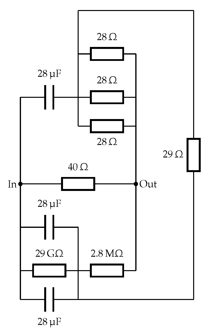
In order to be able to evaluate an EEC produced in the GE process, one needs to build a SPICE netlist from a binary string, which is then evaluated in the SPICE simulator. Standard components (i.e., resistors and capacitors) as well as the EIS specific ZARC element are employed to build EECs. Each component has at least two parameters—the numbers of the connecting ports and the element value(s) (i.e., resistances, capaticances, etc.). This is the BNF used to produce a SPICE netlist:

$$\begin{array}{cc}\hfill N& =\left\{\mathrm{netlist},\mathrm{part},\mathrm{res},\mathrm{cap},\mathrm{zarc},\mathrm{num},\exp ,\mathrm{zexp},\mathrm{znum},\mathrm{gpair}\right\}\hfill \end{array}$$

(1)

$$\begin{array}{cc}\hfill T& =\{0,1,2,3,4,5,6,7,8,9,12,\mathrm{input},\mathrm{output}\}\hfill \end{array}$$

(2)

$$\begin{array}{cc}\hfill S& =\left\{\mathrm{netlist}\right\}\hfill \end{array}$$

(3)

and P is summarized in

Table 1. Production rules.

Nonterminal	Expands to
<netlist>	twelve space separated <part> nonterminals
<part>	<res> | <cap> | <zarc> | None
<res>	rXX (<gpair>) <num><num>e<exp>
<cap>	cXX (<gpair>) <num><num>e-<exp>
<zarc>	aXX (<gpair>) zarcX .model zarcY zarc
	(r=<num>e<exp>
	tau=<num>e-<zexp>n=0.<znum><num>)
<num>	1 | 2 | 3 | 4 | 5 | 6 | 7 | 8 | 9 | 0
<exp>	0 | 3 | 6 | 9 | 12
<zexp>	1 | 2 | 3 | 4 | 5
<znum>	5 | 6 | 7 | 8 | 9
<gpair>	input 1 | input 2 | input 3 | input 4 | input output |
	1 2 | 1 3 | 1 4 | 1 output |
	2 3 | 2 4 | 2 output |
	3 4 | 3 output |
	4 output

.

The first row in the table contains a production rule for the <netlist> nonterminal. The rule ensures that a netlist is composed of up to twelve circuit elements (or parts), separated by spaces. This was performed to prevent bloating (i.e., the uncontrolled growth of the size of a circuit due to unnecessary parallel/serial elements). The second row shows that each of the twelve elements (parts) can become either one of the three actual elements (i.e., resistor, capacitor, or ZARC) or a nonexistent element (None). It can be observed from the next three rows how the three elements are specified. They contain two connecting ports (determined by the <gpair> rule) and the value(s) appropriate for a specific element. A ZARC element contains specialized numeric values (zexp and znum). These are obtained according to expert knowledge (as described in [4,5,23]) in order to narrow down the solution search space. For example, as we are especially interested in the capacitive characteristic of electrochemical processes, we only allow ZARC elements with n between $0.50$ and $0.99$.

Table 2. Feasible value ranges.

Parameter	Value Range
Resistance	[1 $\Omega$, 99 T$\Omega$]
Capacitance	[99 pF, 99 F]
ZARC resistance	[1 $\Omega$, 9 T$\Omega$]
ZARC n factor	[$0.50$, $0.99$]
ZARC time constant	[$9\times {10}^{-9}$ s, $9\times {10}^{-1}$ s]

shows the value ranges of the elements that can be produced using the rules from Table 1.

The last row of Table 1 contains another hard-wired optimization. Instead of specifying each connection port separately, the <gpair> production rule was created which holds all the feasible port combinations (thus, producing some so-called composite terminals made up from terminals from (2)). In that way, two benefits were achieved—a higher chance of creating a working circuit (i.e., where one actually receives a signal from input to output) and a significantly lower chance of creating an illegal circuit with closed loops.

Note that there is still a certain (small) probability that the algorithm produces an invalid circuit when using the above rules—in some conditions, the process of mapping the codons to the actual circuit can result in an element that is connected to itself. Such a circuit can create serious problems during the simulation (i.e., the simulator could either crash or become stuck in an endless loop). In order to avoid such situations, the system was augmented with a special subroutine that detects such circuits and simply eliminates them from the evolutionary process even before they become evaluated for their fitness. Some may argue that this is not the best possible strategy since it may result in a loss of important genetic material at the beginning of the run. That being said, this was still the most efficient solution. Devising a set of production rules that would prevent this problem is simply not feasible.

2.2. Mapping Process Examples

For convenience, we now present two examples of mapping an individual produced during the evolutionary process to an actual electrical circuit.

2.2.1. A Single Element Example

Let us start with a simple example of mapping a chromosome to a single element. Assume one has a chromosome $\{12,127,209,21,76\}$ that they want to map to a single element using the grammar from Section 2.1. Note that, as the chromosome is to be mapped to a single element, rather than a complete netlist, the start symbol will be S = {part}. The goal is to map the start symbol onto terminals by reading codons (i.e., integer values) from a chromosome from which a corresponding production rule is selected by using the following modulo operation.

(rule number) =

(codon integer value) mod

(number of rules for the current nonterminal)

As the start symbol has four possible rules as shown in the second row of Table 1, the codon value of 12 selects the first production rule (i.e., 12 mod $4=0$), hence choosing a resistor. The remaining four codons are then used to map the four nonterminals contained in the production rule for <res> to the corresponding four terminals. The entire mapping process is summarized in

Table 3. Using the chromosome $\{12,127,209,21,76\}$ to map the start symbol <part> to an actual circuit element.

		Number of Rules/	Selected
Codon	Nonterminal	Resulting Rule	Terminal
12	<part>	4/0	<res>
127	<gpair>	15/7	1 4
209	<num>	10/9	0
21	<num>	10/1	2
76	<exp>	5/1	3

. The first column lists the complete chromosome, while the right operands and results of the modulo operations are given in the third column. The last column provides the actual selected terminals by using the corresponding production rule on nonterminals in the second row.

The resulting element is a resistor connected to ports 1 and 4 with a resistance value of 2 k$\Omega$ (i.e., rXX (1 4) 02e3).

2.2.2. A Complete Netlist

The previous subsection illustrated a simple procedure of mapping a chromosome to a single circuit. For the next example, we take a chromosome that came out as the best solution while approximating a Randles circuit. The chromosome is listed in

Table 4. An example chromosome.

236	143	231	47	145	125	33	201	237	187	180
104	251	217	172	112	143	31	227	45	228	183
101	218	83	152	4	253	220	215	77	183	51
147	32	220	173	31	177	0	113	30	211	157
212	45	22	201	117	230	223	171	89	143	243
135	135	11	37	178	161	139	191	148	208	219
159	200	196	231	252	254	232	183	119	165	156
219	205	138	254	133	123	96	68	204	77	229
114	116	139	219	189	97	32	101	166	140	98
168	220	198	93	146	129	130	194	6	125	236
32	51	68	20	183	249	96	156	28	12	62
104	253	104	174	65	11	185	37	137	26	238
86	103	58	122	110	80	222	83	125	18	163
73	19	255	85	104	149	105	127	189	218	54
198	183	144	162	161	47	77	56	21	9	15
16	66	34	132	101	150	135	192	184	138	134
96	96	183	212	147	3	196	101	246	9	241
156	109	113	254	115	13	35	48	117	65	141
8	21	229	74	100	222	69	23	90	7	42
168	120	227	206	147	139	190	22	127	148	187
45	235	97	36	192	92	254	64	188	247	51
183	194	164	61	121	188	100	58	226	255	137
16	88	223	148	155	225	28	233	120	222	167
246	216	225	163	2	86	52	189	45	232	159
118	165	172	74	151	80	19	219	141	0	22
129	33	190	184	253	248	205	30	186	6	186
84	71	126	199	133	127	180	172	159	166	71
27	105	189.

. Using the production rules from Table 1 and start symbol S = {netlist}, one starts with the first codon (236) and perform a modulo 4 operation (the <part> symbol has four possible values) in order to obtain the result 0. As a result, the first of the 12 <part> nonterminals is replaced by the <res> nonterminal, which further expands to 4 nonterminals, the first of which is <gpair>. The next codon (143) maps this nonterminal to the composite terminal (1 output) (obtained as 143 mod 15, which results in rule number 8). The next three codons (231, 47, and 145) determine the numeric value (two digits and exponent) of the resistor. The digits require modulo 10 and exponent modulo 5. The result is a 28 $\Omega$ (i.e., 28e0) resistor. This completes the current element, which means that one moves onto the next <part> nonterminal at the start symbol. The next codon in the sequence (125) selects a capacitor. Following this procedure, a total of 50 codons are used to create a netlist of ten circuit elements as shown in Figure 1. The next two codons (223 and 171 found in the fifth row of Table 4) result in two empty elements (the value of “None”) that are omitted from the netlist. The final netlist and its resulting circuit are shown in Figure 1 and Figure 2, respectively.

2.3. Genetic Operations and Circuits

Evolutionary computation features several operators used to manipulate and combine individual solutions. For the purposes of working with EEC, these operators have to be adjusted accordingly, most noticeably mutation and crossover.

2.3.1. Circuit Mutation

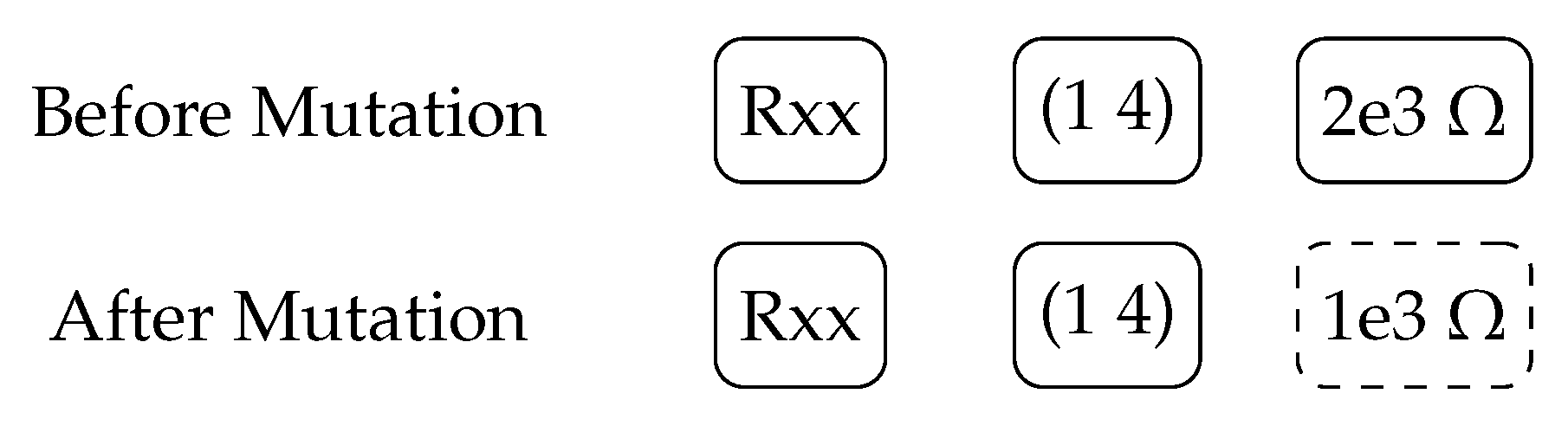
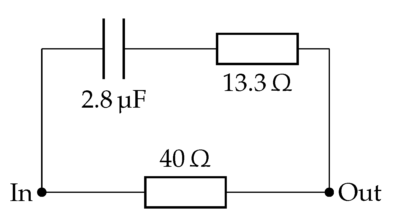
Mutation results in a change in the chromosome of the individual, which is reflected in the final interpretation of the chromosome. The change can be minor or major depending on which codon is selected to mutate. A minor change occurs when, for example, a chromosome from Section 2.2.1 changes from {12, 127, 209, 21, 76} to {12, 127, 209, 70, 76}. The effect of this change is that the resistor changes its value from two kiloohms to one kiloohm, as shown in Figure 3.

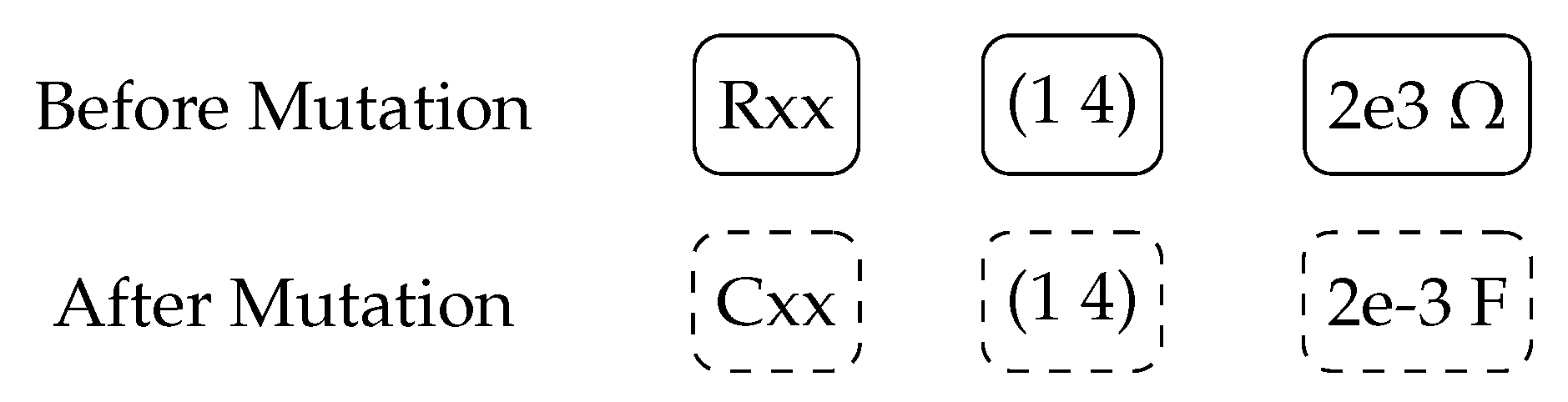
A more significant mutation, on the other hand, happens if the chromosome changes to {117, 127, 209, 21, 76}. That changes a resistor to a capacitor, as shown in Figure 4, which can of course result in a completely different function of the resulting circuit (which is not necessarily a bad thing).

An even more drastic mutation occurs if the same element changes to {119, 127, 209, 21, 76}. This string now represents two empty elements (119 and 127 both map to rule number 3, None), and the next codon (209) is used to determine the next element in the circuit, which will be a capacitor connected to ports 1 and 3 (mapped from <gpair> using the codon with the value of 21).

2.3.2. Circuit Crossover

While mutation targets a single circuit, crossover takes two different circuits (parents) and swaps their elements in order to create new circuits (children) that might be better suited to solving the given problem.

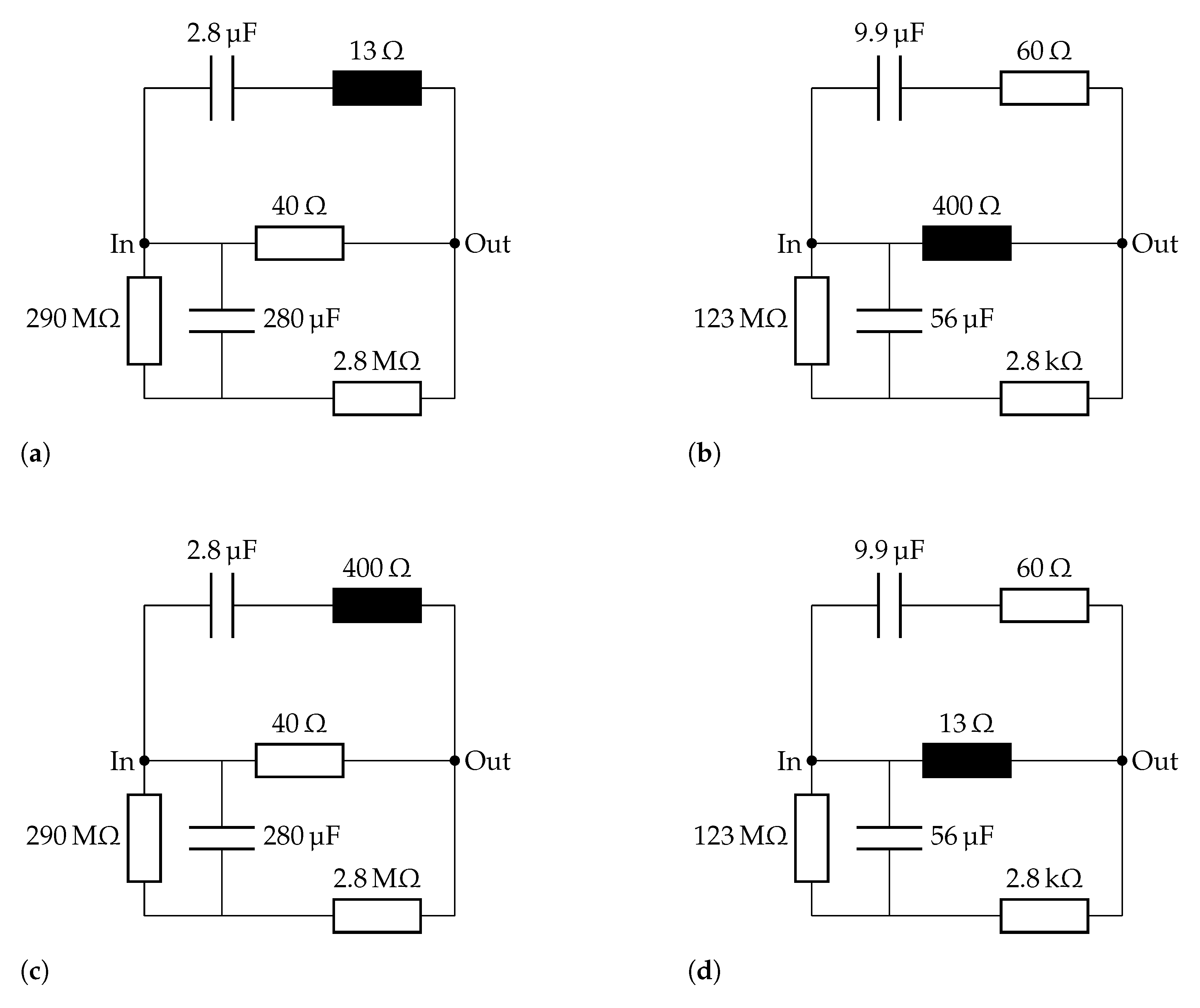
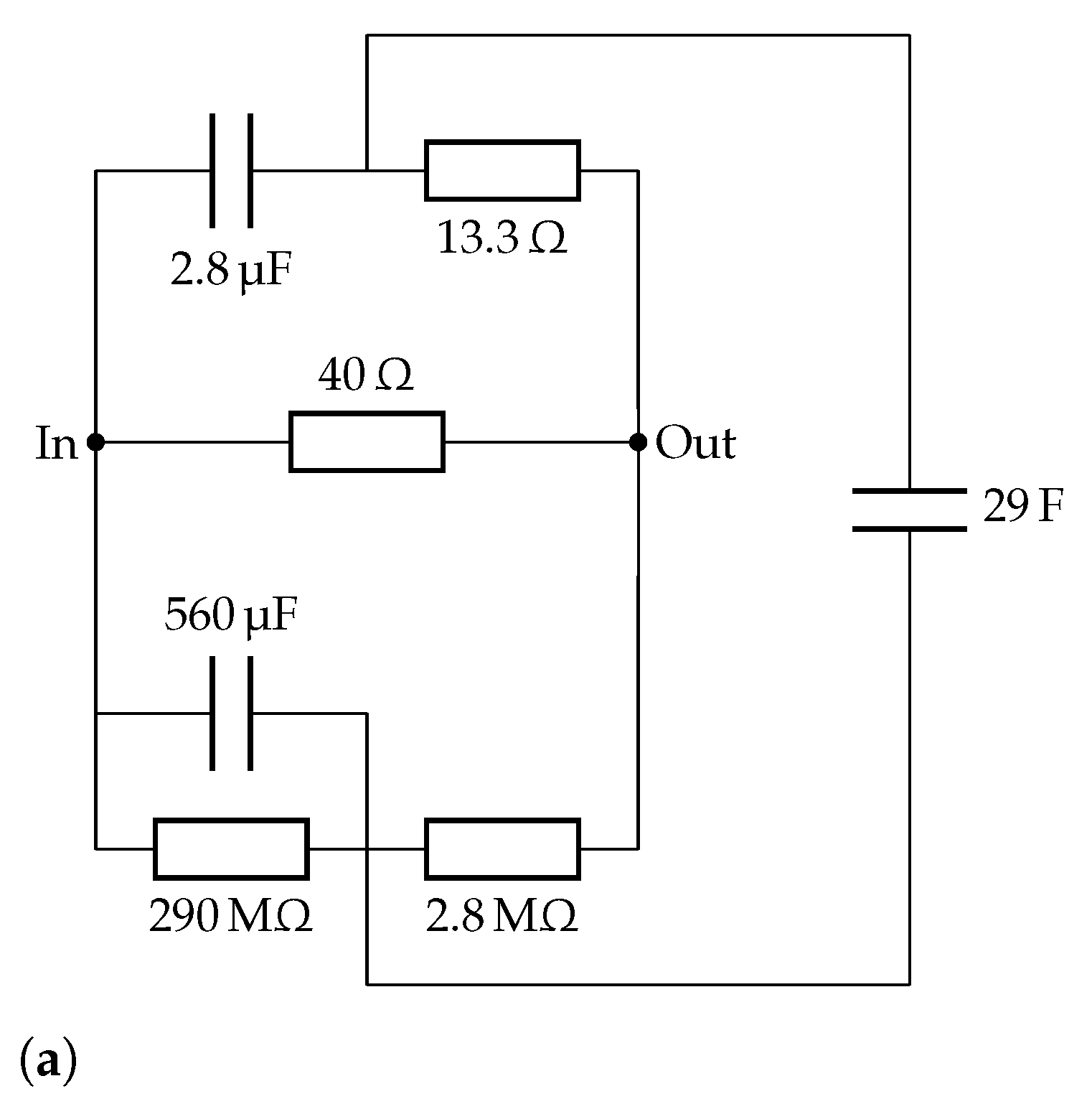
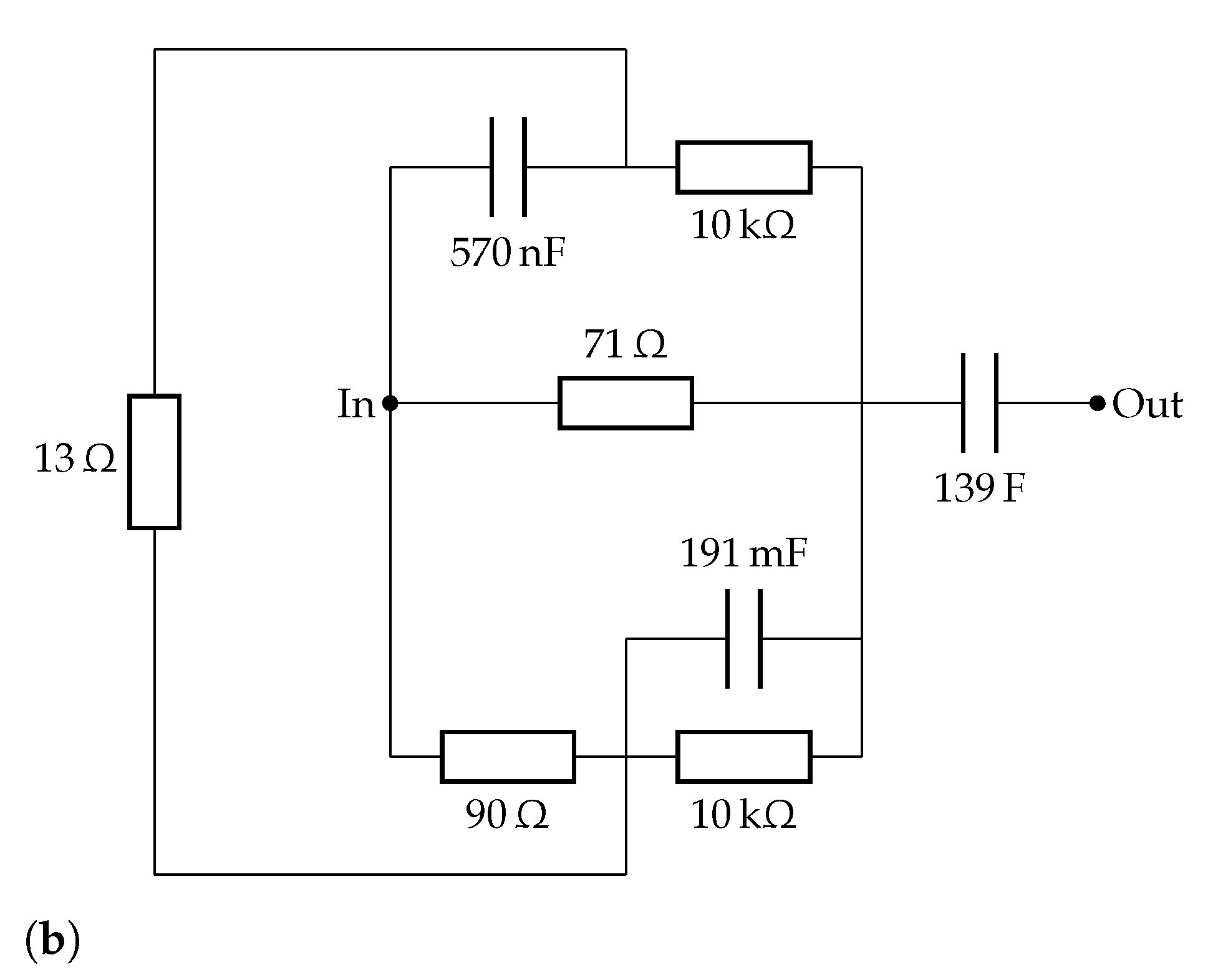
The system first selects two appropriate circuits (usually the circuits that are amongst the better performing ones). In the example (shown in the top row of Figure 5), there are two circuits with identical topology but different component values. In the first step, a random element from Parent 1 is selected—the 13 $\Omega$ resistor drawn in solid black. The algorithm then searches for a similar element in the second circuit (Parent 2) and finds the 400 $\Omega$ resistor. Since two elements of the same type could be found, the crossover can proceed and the two elements are swapped. The chromosomes are adjusted accordingly so as to reflect the change. The resulting circuits (show in the bottom row of Figure 5) are then used as potential candidates in the next generation and (hopefully) perform better than their parents.

Note that we used a slightly modified version of crossover, which focuses on the phenotype instead of considering all available codons. Usually, crossover selects two completely random codons (or substrings of codons) and swaps them. This proved to be quite destructive for the circuits as it usually resulted in the circuit becoming nonfunctional either due to disconnected elements, impossible values, short circuits, or other similar drastic changes. Therefore, we limited the crossover to elements and values in order to preserve circuit integrity and increase the chance of converging towards a working solution.

3. Experiments and Data

Table 5. Genetic parameters used in the experiments.

Parameter	Description
Population Size	300
Generations	250
Mutation type	Fixed Mutation probability
Mutation chance	5%
Fitness	Sheppard’s Objective Function
Elitism	Best individual always survives
Elite size	60% of population

shows the GE parameters that were used in the experiments. The parameters were chosen based on the previous experience with automatic creation of electronic circuits using this method [21]. For this research, we selected Sheppard’s objective [27] function as it is commonly used by researchers for EEC fitting purposes (see, for example, [11]), which makes it easier to compare the results with those in the literature.

3.1. Objective Function and Evaluation

An objective function is used to calculate the cost or fitness of a solution. The cost of an individual reflects how well the individual solves a given problem—the lower the cost the closer the solution to the desired behavior. How the objective function is selected and/or constructed depends strongly on the problem at hand. In some cases, the objective function represents a simple numerical comparison of points between two curves while it can be a complex multi-objective function in others that compares different aspects of the solution such as cut-off frequency, damping, gain, and combines them into a single measure.

Sheppard’s Objective Function

It was already mentioned that, in the experiments, we employed the objective function proposed by Sheppard et al. [27], which is commonly used for solving Complex Nonlinear Least Squares (CNLS) problems (e.g., [8,11]).

$$\begin{array}{cc}\hfill S& =\sum _{j=1}^m(w_j{(Re(y_j^{exp})-Re(y_j^{com}))}^2+w_j{(Im(y_j^{exp})-Im(y_j^{com}))}^2),\hfill \end{array}$$

(4)

$$\begin{array}{cc}\hfill w_j& =\frac{1}{Re{(y_j^{exp})}^2+Im{(y_j^{exp})}^2}.\hfill \end{array}$$

(5)

Here, $m,y_j^{exp},y_j^{com},\mathrm{and}{w}_j$ are the number of data points, the jth value of experimental impedance data to be fitted, the jth value of impedance data computed by the proposed algorithm, and the weighting modulus factor [28] associated with the jth data point. The goal of the evolutionary algorithm is to minimise the value of S.

3.2. Data Sets Used for Evaluation

The experimental impedance data to be fitted were obtained either via mathematical models (so-called synthetic data) or from measurements in a realistic environment [5].

3.2.1. Randles Circuits

The first two sets of synthetic data were generated using two circuits that contain only resistors and capacitors, without any constant phase elements. The first of the two circuits contains three elements (an equivalent of one Randles circuit [23]), and the second one contains five elements (an equivalent of two serially linked Randles circuits). The impedance characteristics and the corresponding Randles circuits can be observed in Figure 6 and Figure 7.

3.2.2. Cole–Cole Model

A more complex Cole–Cole (ZARC) [29] model was employed for the next set of synthetic data. This model is widely used in Distribution of Relaxation Time (DRT) studies [3,4,5] and can also be applied when developing new algorithms for solving CNLS problems [13]. The following equation was used to compute single (K = 1) and double (K = 2) ZARC element data:

$$Z_{ZARC}({\omega }_j)=\sum _{k=1}^{k=K}\frac{R_k}{1+{(i{\omega }_j{\tau }_{0,k})}^{n_k}},k=1,2,...,N,$$

(6)

where ${\omega }_j$ is an angular frequency associated with the jth impedance data point, i is the imaginary unit, $R_{\mathit{k}}$ is the kth resistance, $n_k$ is a factor related to a constant phase element [11], and ${\tau }_{0,\mathit{k}}$ is the kth time constant.

ZARC data in this study were computed by using (6) and values in

Table 6. Parameters used to compute single and double ZARC data.

Synthetic Data	${\mathit{R}}_1(\mathbf{\Omega }{\mathbf{cm}}^2)$	${\mathit{\tau }}_{0,1}(\mathit{s})$	${\mathit{n}}_1$	${\mathit{R}}_2(\mathbf{\Omega }{\mathbf{cm}}^2)$	${\mathit{\tau }}_{0,2}(\mathit{s})$	${\mathit{n}}_2$
ZARC	50	0.01	0.7	50	0.0001	0.7

. An example of such synthetic data can be observed in Figure 8 where a double ZARC (i.e., $k=2$) was used to generate the impedance characteristic. This characteristic is defined by two suppressed semi-circuits that can be frequently found in EIS study [5,30].

3.2.3. Solid Oxide Fuel Cell Data

Realistic data were obtained from the measurements of solid oxide fuel cells, which were already used in the previous work [5]. The measured cells were industrial-sized and characterized by an active surface of 80 cm${}^2$ and an operating temperature of 800 °C. Humidified hydrogen was used as a fuel for a fuel electrode, and air was used as fuel for an air electrode. More details regarding the experimental setup can be found in [31]. The impedance characteristic obtained from the measurements is shown in Figure 9.

Note that, compared to synthetic data, this set features a lot less comparison points since it was obtained from real measurements. We were, therefore, faced with two options—either to evaluate the model using only the original data points or try to increase the amount of points using interpolation. We opted for interpolation since it permits better accuracy with respect to the evaluation of the results (more data points help to match the curve with better accuracy). We used the linear interpolation included in the Numpy Python package. Incidentally, without interpolation, the algorithm was unable to evolve an appropriate EEC since almost any random circuit fitted in the original twenty data points quite well. Using interpolation, every single run produced an acceptable solution.

4. Results

This section presents the results of running the grammatical evolution algorithm in trying to approximate the data provided in the previous section.

4.1. Randles Impedance Characteristic Matching

After initial fiddling with system settings and parameters (maximum number of elements and a few others), the system was able to consistently produce matching circuits with a good fit with the Sheppard’s value of $0.29$ or lower. What is more, at least half of the population (i.e., 150 circuits) produced viable (and different) solutions, which means that the system is able to produce several candidates in a single run. Figure 10 and Figure 11 show that the matched impedance characteristics (dashed orange) overlaid over the original (solid blue) characteristic and layouts of the best matching circuits for each case, respectively.

Note that the presented approach generates some additional elements that can be later removed with a bit of expert knowledge. An example of such a simplification is shown in Figure 12, where the elements that have no effect since they are too large to receive any current were removed. Thus, the capacitor with 29 F was removed since it is effectively an open circuit, and no current passes through it at measured frequencies. The entire bottom subcircuit (the two resistors of 290 MΩ and 2.8 MΩ and the 560 μF capacitor) can also be removed since there will be no current over these elements as there is a path with much lower resistance (i.e., via the 13.3 Ω and 40 Ω resistors).

4.2. Cole–Cole Fitting

Cole–Cole data revealed a serious problem with the system—any simulation with a $n_k$ factor lower than $0.9$ failed to produce a working circuit. However, this is not a surprise as such a factor requires a Constant Phase Element (CPE) in order to be included in a circuit and in order for the circuit to be able to produce the desired characteristic. Note that a CPE features frequency dependant values, which cannot be carried out using basic electronic components (i.e., resistors and capacitors) nor does such an element exist in the SPICE simulator. Fortunately, SPICE lends itself to implementing and integrating custom circuit elements; therefore, we created a model for the ZARC element based on (6) and added it to the Spice Opus circuit simulator as a built-in device. The model was implemented via the XSPICE extensions, which allow the user to load user-defined devices from dll files. However, because EIS only requires a small-signal AC analysis, a transient analysis model was omitted because of its undue complexity and the fact that it is not needed in the simulations. It is quite crucial that we built this model since it enabled us to continue to use the SPICE simulator. We believe this is the first implementation of the ZARC element in SPICE since we have not found it mentioned anywhere in the literature.

The results obtained with the updated engine are once again spot on, as observed in Figure 13.

The resulting circuit is shown in Figure 14 with ZARC values provided in

Table 7. ZARC values for the elements in circuit from Figure 14.

Element	$\mathit{R} (\mathbf{\Omega }{\mathbf{cm}}^2)$	$\mathit{\tau } (\mathbf{s})$	n
ZARC1	348.21	0.0003	0.91
ZARC2	65	0.065	0.53
ZARC3	66	0.003	0.57
ZARC4	80	0.00005	0.5

. Again, the circuit was simplified (by removing unnecessary parallel/serial resistors and capacitors), but the resulting circuit still differs from the expected topology of two serial ZARC elements. The issue here lies in the fact that the presented system creates a circuit with a fitting impedance characteristic and matching time constants. It succeeds in this task since the results (extracted via Python Cole–Cole decomposition) indicate that the resulting circuit (Figure 14) yields time constants values ($0.007$ and $0.00008$) that are close to the ones ($0.01$ and $0.0001$) used to prepare the original data (see Table 6). The final metric value is, therefore, slightly larger in the range of 10 due to a more complex problem (multiple ZARC elements), but the resulting circuit meets the expectations. We believe that this value could be further lowered with further fine tuning of the parameters, such as increasing the accuracy of element values (from two digits two four, using all possible exponent values, and increasing the number of generations in our experiment).

4.3. Solid Oxide Fuel Cell Fitting

As already noted in the last paragraph of Section 3, additional comparison points using interpolation had to be generated because the measured points were too few for the algorithm to be able to find a matching circuit. Taking more measured data points requires extra time, which prolongs DRT analysis that is vital for monitoring SOFC health. After the interpolation, the best obtained matching impedance characteristic is demonstrated in Figure 15, with the dashed line representing the fitted characteristic. Please note that the line appears smoother since it was generated via an AC sweep, while the original characteristic (solid line) comes from connecting the original (fewer) data points. Nevertheless, the characteristic was fitted with the Sheppards value of 300 and we believe that—if we had more measured data points available—the Sheppards value would be lower due to the disuse of interpolation.

The resulting circuit (shown in Figure 16) is fairly simple given the complexity of input data. Regardless, a fitting circuit and DRFT characteristic was found without much trouble beyond interpolating the data points. This is significant since it opens many new possibilities of quickly fitting measured data and finding the relevant time constants.

5. Discussion

Grammatical evolution was used as an automatic method for creating a matching EEC circuit without much additional user input. Basically, the research started from previous work conducted on evolving electrical circuits [21], which turned out to be quite appropriate for the problem at hand. Amongst the most important additions that had to be implemented for this research was modified grammar, a new metric, and the implementation of a new element for the SPICE simulator.

In a series of experiments, we successfully created several solutions that fitted the supplied data—synthetic as well as real—with a sufficient level of accuracy. Some of the resulting circuits were similar to the known EEC solutions while others present a possible new standard model that should be further investigated by experts in the EIS field.

We believe that the presented approach offers at least two important benefits. Firstly, it automates the EEC creation process and renders the entire method accessible even to less experienced researchers who are only starting in this field. Secondly, it might produce new standard EEC circuits and help identify new, previously overlooked ongoing electrochemical processes.

References

1. Barsoukov, E.; Macdonald, J.R. Impedance Spectroscopy: Theory, Experiment, and Applications; Wiley: Hoboken, NJ, USA, 2005. [Google Scholar]
2. Yuan, X.Z.; Song, C.; Wang, H.; Zhang, J. EIS Applications. In Electrochemical Impedance Spectroscopy in PEM Fuel Cells: Fundamentals and Applications; Springer: London, UK, 2010; pp. 263–345. [Google Scholar] [CrossRef]
3. Wan, T.H.; Saccoccio, M.; Chen, C.; Ciucci, F. Influence of the Discretization Methods on the Distribution of Relaxation Times Deconvolution: Implementing Radial Basis Functions with DRTtools. Electrochim. Acta 2015, 184, 483–499. [Google Scholar] [CrossRef]
4. Dion, F.; Lasia, A. The use of regularization methods in the deconvolution of underlying distributions in electrochemical processes. J. Electroanal. Chem. 1999, 475, 28–37. [Google Scholar] [CrossRef]
5. Zic, M.; Pereverzyev, S., Jr.; Subotic, V.; Pereverzyev, S. Adaptive multi-parameter regularization approach to construct the distribution function of relaxation times. Gem-Int. J. Geomath. 2020, 11, 1–23. [Google Scholar] [CrossRef] [Green Version]
6. Song, J.; Bazant, M. Electrochemical Impedance Imaging via the Distribution of Diffusion Times. Phys. Rev. Lett. 2018, 120, 116001. [Google Scholar] [CrossRef] [PubMed] [Green Version]
7. Pereverzev, S.V.; Solodky, S.G.; Vasylyk, V.B.; Žic, M. Regularized Collocation in Distribution of Diffusion Times Applied to Electrochemical Impedance Spectroscopy. Comput. Methods Appl. Math. 2020, 20, 517–530. [Google Scholar] [CrossRef]
8. Boukamp, B.A. A nonlinear least-squares fit procedure for analysis of immittance data of electrochemical systems. Solid State Ionics 1986, 20, 31–44. [Google Scholar] [CrossRef] [Green Version]
9. Macdonald, J.R.; Schoonman, J.; Lehnen, A.P. The applicability and power of complex non-linear least-squares for the analysis of impedance and admittance data. J. Electroanal. Chem. 1982, 131, 77–95. [Google Scholar] [CrossRef]
10. Sihvo, J.; Roinila, T.; Stroe, D.I. Novel Fitting Algorithm for Parametrization of Equivalent Circuit Model of Li-Ion Battery from Broadband Impedance Measurements. IEEE Trans. Ind. Electron. 2021, 68, 4916–4926. [Google Scholar] [CrossRef]
11. Žic, M. An alternative approach to solve complex nonlinear least-squares problems. J. Electroanal. Chem. 2016, 760, 85–96. [Google Scholar] [CrossRef]
12. Kobayashi, K.; Suzuki, T. Development of impedance analysis software implementing a support function to find good initial guess using an interactive graphical user interface. Electrochemistry 2020, 88, 39–44. [Google Scholar] [CrossRef] [Green Version]
13. Žic, M.; Subotić, V.; Pereverzyev, S.; Fajfar, I. Solving CNLS problems using Levenberg-Marquardt algorithm: A new fitting strategy combining limits and a symbolic Jacobian matrix. J. Electroanal. Chem. 2020, 866, 114171. [Google Scholar] [CrossRef]
14. Lan, C.; Liao, Y.; Hu, G. A unified equivalent circuit and impedance analysis method for galloping piezoelectric energy harvesters. Mech. Syst. Signal Process. 2022, 165, 108339. [Google Scholar] [CrossRef]
15. Zic, M. Optimizing Noisy CNLS Problems by Using the Adaptive Nelder-Mead Algorithm: A New Approach to Escape from Local Minima. 2018. Available online: https://ricamwww.ricam.oeaw.ac.at/files/reports/18/rep18-22.pdf (accessed on 19 October 2021).
16. Levenberg, K. A method for the solution of certain non-linear problems in least squares. Q. Appl. Math. 1944, 2, 164–168. [Google Scholar] [CrossRef] [Green Version]
17. Marquardt, D.W. An algorithm for least-squares estimation of nonlinear parameters. J. Soc. Ind. Appl. Math. 1963, 11, 431–441. [Google Scholar] [CrossRef]
18. Moré, J. The Levenberg-Marquardt algorithm: Implementation and theory. In Numerical Analysis; Lecture Notes in Mathematics; Watson, G., Ed.; Springer: Berlin/Heidelberg, Germany, 1978; Volume 630, pp. 105–116. [Google Scholar] [CrossRef] [Green Version]
19. Nelder, J.A.; Mead, R. A Simplex Method for Function Minimization. Comput. J. 1965, 7, 308–313. [Google Scholar] [CrossRef]
20. Dellis, J.L.; Carpentier, J.L. Nelder and Mead algorithm in impedance spectra fitting. Solid State Ionics 1993, 62, 119–123. [Google Scholar] [CrossRef]
21. Kunaver, M. Grammatical Evolution-based Analog Circuit Synthesis. Inf. MIDEM 2019, 49, 229–239. [Google Scholar]
22. O’Neil, M.; Ryan, C. Grammatical Evolution. In Grammatical Evolution: Evolutionary Automatic Programming in an Arbitrary Language; Springer: Boston, MA, USA, 2003; pp. 33–47. [Google Scholar] [CrossRef]
23. Macdonald, J.R. Impedance spectroscopy: Models, data fitting, and analysis. Solid State Ionics 2005, 176, 1961–1969. [Google Scholar] [CrossRef]
24. Tuinenga, P.W. SPICE: A Guide to Circuit Simulation and Analysis Using PSpice, 1st ed.; Prentice Hall: Englewood Cliffs, NJ, USA, 1988. [Google Scholar]
25. Kunaver, M.; Fajfar, I. Grammatical Evolution in a Matrix Factorization Recommender System. In International Conference on Artificial Intelligence and Soft Computing; Rutkowski, L., Korytkowski, M., Scherer, R., Tadeusiewicz, R., Zadeh, L.A., Zurada, J.M., Eds.; Lecture Notes in Computer Science; Springer: Berlin/Heidelberg, Germany, 2016; Volume 9692, pp. 392–400. [Google Scholar] [CrossRef]
26. Naur, P. Revised Report on the Algorithmic Language Algol 60. Commun. ACM 1963, 6, 1–23. [Google Scholar]
27. Sheppard, R.J.; Jordan, B.P.; Grant, E.H. Least squares analysis of complex data with applications to permittivity measurements. J. Phys. D Appl. Phys. 1970, 3, 1759–1764. [Google Scholar] [CrossRef]
28. Zoltowski, P. The error function for fitting of models to immittance data. J. Electroanal. Chem. 1984, 178, 11–19. [Google Scholar] [CrossRef]
29. Cole, K.S.; Cole, R.H. Dispersion and absorption in dielectrics I. Alternating current characteristics. J. Chem. Phys. 1941, 9, 341–351. [Google Scholar] [CrossRef] [Green Version]
30. Žic, M.; Fajfar, I.; Subotić, V.; Pereverzyev, S.; Kunaver, M. Investigation of Electrochemical Processes in Solid Oxide Fuel Cells by Modified Levenberg–Marquardt Algorithm: A New Automatic Update Limit Strategy. Processes 2021, 9, 108. [Google Scholar] [CrossRef]
31. Subotić, V.; Stoeckl, B.; Lawlor, V.; Strasser, J.; Schroettner, H.; Hochenauer, C. Towards a practical tool for online monitoring of solid oxide fuel cell operation: An experimental study and application of advanced data analysis approaches. Appl. Energy 2018, 222, 748–761. [Google Scholar] [CrossRef]
Scheme 1. Different approaches commonly applied in EIS study.
Processes 09 01859 sch001
Figure 1. A netlist created from the chromosome from Table 4.
Processes 09 01859 g001
Figure 2. The final circuit from the chromosome from Table 4.
Processes 09 01859 g002
Figure 3. A minor circuit mutation where only the value of the element changes (dashed).
Processes 09 01859 g003
Figure 4. A more serious circuit mutation where the type of the element changes (dashed).
Processes 09 01859 g004
Figure 5. Two circuits before (parents) and after (children) crossover. (a) Parent 1; (b) Parent 2; (c) Child 1; (d) Child 2.
Processes 09 01859 g005
Figure 6. Single ZARC characteristic and its equivalent circuit. (a) Z characteristic; (b) Equivalent circuit.
Processes 09 01859 g006
Figure 7. Double ZARC characteristic and its equivalent circuit. (a) Z characteristic; (b) Equivalent circuit.
Processes 09 01859 g007
Figure 8. Double ZARC synthetic data characteristic.
Processes 09 01859 g008
Figure 9. Solid oxide fuel cell characteristic—measured data.
Processes 09 01859 g009
Figure 10. Randles circuit—matched impedance characteristic. (a) Single; (b) Double.
Processes 09 01859 g010
Figure 11. Randles fitted circuits. (a) Single; (b) Double.
Processes 09 01859 g011aProcesses 09 01859 g011b
Figure 12. A simplified circuit from Figure 11a.
Processes 09 01859 g012
Figure 13. The result of fitting the synthetic data obtained using the Cole–Cole equation (i.e., ZARC elements).
Processes 09 01859 g013
Figure 14. Cole–Cole fitted circuit.
Processes 09 01859 g014
Figure 15. Solid oxide fuel cell fitted impedance characteristic.
Processes 09 01859 g015
Figure 16. Fuel cell simplified fitted circuit.
Processes 09 01859 g016