Incorporating Environmental Perspective in Integrated Strategic-Tactical Economic Optimization Model of Biomass-to-Biofuel Supply Chain—A Real Case Study in Ethiopia

Abstract

Several optimization models, which consider economic and environmental perspectives, have been developed recently to support the sustainable biomass-to-biofuel supply chain (BBSC) design. All of the economic-environmental optimization models rely on solving long-term planning problems with a conventional hierarchical approach, where tactical decisions are made based on the optimal strategic decisions from the strategic-level model, despite it arousing non-optimal solutions. Moreover, almost all of them have used non-monetary-based environmental indicators, which result in difficulties with clarity when comparing with economic objectives. Therefore, in this work, an effort is made to develop a more reliable planning strategy that offers optimal strategic and tactical decisions simultaneously and maximizes the economic and environmental benefits. Furthermore, the environmental performance of the BBSC has been assessed in terms of monetary value by adopting an ecocost approach after performing an LCA on the system. The integrated model is applied in the real biofuel sector of Ethiopia to optimize the country’s bioethanol and biodiesel supply chain over a 20-year horizon. Despite the abrupt rise in the model size, with it being a real countrywide case with many variables and large quantities of data, an alternative semi-heuristic method that offers a feasible solution to the multi-objective problem is provided.

1. Introduction

Recent economic trends coupled with the anticipated stringent regulation to blend petroleum products with biofuel will increase the demand for biofuel products in Ethiopia in the near future. Most of the biofuel demand belongs to the transportation sector. The import of petroleum products accounts for a major share of the total import expenditure and consumes about 70% of the total export earnings of the country. In light of the increasing cost of oil and demand for petroleum products, the Ethiopian government has included the development of biofuel as one of its development strategies since 2007. Moreover, one of the main reasons that biofuel has been promoted in Ethiopia is to meet the needs of a green economy, which the country has envisaged reaching by 2030. The Climate Resilient Green Economy (CRGE) strategy of Ethiopia has clearly indicated the significance of biofuel in reducing GHG emissions and meeting the green economy targets of the country [1]. The strategy identified one of the abatement levers for GHG in the transport sector as bioethanol and biodiesel in fuel mixtures. According to the strategy’s assessment, increasing the current 10% bioethanol–gasoline mix to 15% and launching a 5% biodiesel–diesel mix has a reduction potential of 0.2 and 0.7 Mt CO₂eq in 2030, respectively.

Despite the economic, environmental, and social benefits as well as the government’s ambitious plan, biofuel development had been nominal. Bioethanol production is quite low compared with the government’s envisaged plan, and biodiesel production is still at the pilot scale [2]. This is attributed to several challenges that hinder the sector’s progress along the biomass-to-biofuel supply chain (BBSC), in which the economic and environmental challenges are the major barriers to overcome. Furthermore, the non-evidence-based policies related to biofuel have also taken the lion’s share of the underdevelopment of the sector. To address these hurdles, allow policymakers to make evidence-based decisions and plan at strategic and tactical levels throughout the BBSC, quantitative research is imperative.

Cognizant to the above fact, the aim of this work is to develop a decision support economic-environment optimization model for the infant BBSC of Ethiopia, which helps policymakers to make more rational and quantitatively justified decisions or plans. Both strategic and tactical decisions associated with the BBSC over the next 20 planning years are the proposed outcome of the optimization model. This work is an extension of previous work of Tesfamichael et al. [3], which focuses on the economic performance of the BBSC only.

The rest of the article is structured as follows. In the next section, the state-of-the-art of this study is presented after reviewing the research limitations of previous works in this scientific domain. Section 3 provides the model formulation by looking in to the economic and environmental objectives. A detailed mathematical model, which includes all the mass balances and constraints, is presented in Appendix A. Moreover, Section 3 discusses briefly how the case study data are taken and assumed. The multi-objective optimization strategy is presented in Section 4. Section 5 is dedicated to discussing the optimal and feasible results associated with the mono-, bi- and multi-objective optimizations. Finally, conclusions are drawn and future research avenues are recommended.

2. State of the Art

Recently, mathematical optimization-based models have gained a considerable amount of attention to support decision making in different supply chains. In this regard, various optimization studies, focusing on the optimal design of supply chain in general and BBSC in particular, have been conducted in the past decade. The motive of the majority of the models revolves around the economic performance optimization of the BBSC, which is followed by economic-environment performance optimization models [4]. Almost all of the environment optimization models have used non-monetary-based indicators, which results in difficulty comparing the economic objectives in a clear manner. The most frequently used environmental indicators are tons of GHG emission per ton of material, e.g., [5,6], tons of GHG savings per ton of material, e.g., [7], eco-indicator-99 per ton of material, e.g., [8,9], and environmental impacts per ton of material, e.g., [10]. A recent study by Zore et al. [11] had used the ecocost method to convert environmental impact to monetary value, despite the focus of the study not being related to supply chain optimization. Moreover, the study intended to develop a single objective model, which only provides strategic-level decisions [11].

In any design and plan of a supply chain, decision making is hierarchized under three levels: strategic (long term), tactical (medium term), and operational (short term). The prior intention in many of the previous optimization studies was strategic-level planning. A review from Barbosa-Póvoa et al. [12] has shown that, in the 207 optimization models developed in various sectors, almost 70% have focused on the strategic aspects of the supply chain. For example, Lam et al. [13] developed a strategic-level model that intended to minimize the total carbon footprint for the energy supply chain of a region, with a focus on determining the optimal network design of the supply chain. Similarly, the focus of the multi-period MILP model developed by Cucek et al. [14] was a strategic-level planning that determines optimal raw materials, technologies, intermediate and final product flows of a bioenergy supply chain. Despite the strategic-level design is the intention of the above studies as well as other research that focuses on bioenergy supply chain optimization, a decision support model should incorporate at least a tactical level of planning along with a strategic design to be more comprehensive and reliable for policymakers. Next to strategic-level models, around 28% of the optimization models developed so far are applied for the combined strategic-tactical level decisions [12]. The aim of strategic-tactical optimization models is to consolidate long-term (strategic) planning, such as the optimum capacity, technology and location of biorefinery and other facilities of the supply chain, along with medium-term (tactical) planning, such as transportation, material flows, and inventory management. The hierarchical approach is the conventional way of doing the strategic-tactical optimization in almost all studies [15]. In this approach, sub-problems are aroused from a single problem that can be computed independently based on their hierarchy [16], i.e., the basis for the tactical decisions are the results acquired from the strategic-level optimization model. However, recent studies have shown that infeasible and non-optimal solutions may arouse at the tactical level by using the solutions from the strategic-level optimization model. For example, using the hierarchical approach, Akhtari et al. [15] have discovered that the recommended quantity of biomass transported from supply source to conversion unit by the strategic model was not adequate for gaining the monthly biomass requirement of the unit. Moreover, the determined processing capacity of the unit by the strategic model was not enough to acquire the demands for bioenergy in some months. The hierarchical model results of Paradis et al. [17] have also shown the incoherence of tactical- and strategic-level plans, as the model output failed to ensure sustaining supply of wood to meet long-term industrial fiber demand. Moreover, Tesfamichael et al. [3] showed that the implementation of the hierarchical model for the case study considered in this work has emanated infeasibility in some of the results. Based on this study’s results, the recommended capacity of biorefinery that is available in some locations by the strategic model was not enough to produce the expected bioethanol following the pattern of biomass supply per month [3].

Considering the above outcomes of different models, it is mandatory to develop a planning strategy that makes optimal strategic and tactical decisions simultaneously by considering the monthly variations in some of the model parameters such as biomass supply and biofuel demand. However, to the best of our knowledge, very few integrated strategic-tactical models have been developed so far to address the issue of non-optimality and infeasibility. Akhtari et al. [15] have developed an integrated MILP model for the supply chain of forest based biomass to address midterm fluctuation in the demand and supply of biomass, which are mostly overlooked in strategic models. Additionally, Lin et al. [18] developed an integrated model by simultaneously optimizing both tactical and strategic planning decisions with the intention of minimizing annual miscanthus–bioethanol production costs. Moreover, an efficient bioethanol supply chain using swithchgrass as a feedstock was designed through integrated model by Zhang et al. [19]; this model helps to efficiently manage the logistics along with other strategic issues. In parallel, Eksioglu et al. [20] had also proposed an integrated mathematical model for bioethanol supply chain, which is used for supply chain design and biorefinery logistics management. Furthermore, Tesfamichael et al. [3] devised an integrated model, which is designed for long-term BBSC planning that considers both bioethanol and biodiesel produced from five different biomass feedstocks.

However, the intention in all of the above integrated strategic-tactical models revolves only around the economic objectives, for example, the minimization of the annual supply chain costs in [19,20], minimization of the annual production costs in [18], maximization of the net present value (NPV) in [15] and maximization of profit and minimization of investment cost in [3]. Furthermore, as indicated above, the integrated models that focus on biofuel supply chain considers a single biomass feedstock and product (bioethanol) except Tesfamichael et al. [3], who consider multi-feedstock and multi-products (bioethanol and biodiesel) BBSC. Motivated by the drawbacks of the previous research, an effort is made in this paper to develop a multi-objective economic-environment optimization model, which considers the following issues simultaneously:

(a)

An alternative semi-heuristic solution method that offers a feasible solution to the problem is provided as the attempt to solve the multi-objective optimization model with numerical solver ends without success. This is due to the abrupt rise in the size of the model because it is a real, national-level case study with many continuous decision variables and parameters as well as the availability of many binary variables due to strategic choices.

(b)

An integrated model is designed to make optimal or feasible strategic and tactical decisions simultaneously.

(c)

Contrary to many previous research endeavors that emphasize GHG emissions and global warming potential, this study attempts to formulate a comprehensive assessment of BBSC’s environmental impact by broadening the assessed mid-point impact categories. The assessed mid-point categories include global warming, photochemical oxidation, acidification, eutrophication, human toxicity, fine dust, freshwater aquatic ecotoxicity, land use, waste generation, fossil fuel depletion and metal and water scarcity potentials, despite most of them being insignificantly affected by the BBSC activities.

(d)

The environmental impacts are converted to monetary values using the ecocost approach to easily compare economic criteria. The ecocost is the marginal prevention cost required to halt the negative impact of toxic emissions. These emissions are associated with human health as well as ecosystems, emissions that cause global warming, and resource depletion (metals, rare earths, fossil fuels, water, and land use).

Although less structured and more creative eco-design approaches have been emerged recently [21], they fail to provide a quantitative comparison among different objectives. As a result of this, the mathematical model developed here, which offers quantitatively substantiated optimal results, will provide an excellent basis for eco-improvement and eco-innovation, despite its very structured approach with a rigid mathematical formulation.

3. Materials and Methods

3.1. Model Formulation

The concerned problem in this work is the design of BBSC, which includes all the principal supply chain components—upstream and downstream of the biorefineries—for a real case in Ethiopia. The considered components of the supply chain are feedstock supply centers, preprocessing facilities, biorefineries, bioethanol and biodiesel distribution units, and demand zones of bioethanol, biodiesel and co-products. The proposed model will provide feasible strategic and tactical solutions, which may support policymakers while deciding issues pertaining to biofuel sector. Figure 1 presents the superstructure of the BBSC model addressed in this work.

As it is indicated in Figure 1, the BBSC encompasses a set of biomass feedstocks (b∈B) purchased from different supply sources (h∈H) and pretreated using preprocessing units available at a set of candidate locations (i∈I) with a set of technologies (f∈F) and capacities (c∈C) to produce a set of preprocessed biomasses (d∈D). Then, the preprocessed biomasses are converted to a set of biofuel (u∈U) and co-products (v∈V) using refineries available at set candidate locations (j∈J) with a set of technologies (g∈G) and capacities (e∈E). Finally, the produced biofuels are conveyed to distribution centers available at a set of candidate locations (k∈K) with a set of capacities (a∈A) or directly to a set of biofuel markets (m∈M). Additionally, the co-products are directly transported to a set of co-product markets (n∈N). The lifetime of the project is divided in equally sized years (y∈Y) and months (t∈T).

The mathematical model for BBSC is comprised of two economic and one environmental objective function along with numerous constraints. This model is designed for long-term planning studies, in that it is utilized to optimize the BBSC over a 20-year horizon. To plan the strategic and tactical planning levels simultaneously from the feedstock supply centers to the final demand zones, a deterministic mixed-integer linear programming (MILP) model is developed. The problem is a multi-period, multi-feedstock, multi-product, and multi-echelon to entertain the entire nature of the BBSC. Both monthly and yearly time periods are considered in the model. This model, which simultaneously satisfies constraints related to biomass resource, capacity, technology, and demand of biofuel and co-product, has considered both monthly and yearly time periods. Constraints are formulated to integrate these two time periods via inventory levels of biomass, preprocessed biomass, and biofuel to prevent non-optimal and infeasible solutions aroused as a result of segregated decision making for strategic- and tactical-level decisions [15].

The continuous variables of the model are related to production, inventory and transportation of materials in the BBSC, as indicated below. All the continuous variables are in the year y and month t.

Production: Wbif_b,d,i,f,y,t—the quantity of feedstock b converted to preprocessed feedstock din preprocessing unit located at i using technology f. Wdif_b,d,i,f,y,t—the quantity of preprocessed feedstock d obtained from feedstock b in preprocessing unit located at i using technology f. Wdjg_d,u,j,g,y,t—the quantity of preprocessed feedstock d converted to biofuel u in biorefinery located at j via technology g. Wujg_d,u,j,g,y,t—the quantity of biofuel u obtained from preprocessed feedstock d in biorefinery located at j via technology g. Wvjg_d,v,j,g,y,t—the quantity of coproduct v obtained from preprocessed preprocessed feedstock d in biorefinery located at j via technology g.

Inventory: Inventory amount of feedstock b at preprocessing center i (IVBI_b,i,y,t), processed feedstock d at preprocessing facility i (IVDI_d,i,y,t), preprocessed feedstock d at biorefinery j (IVDJ_d,j,y,t), biofuel u at biorefinery j (IVUJ_u,j,y,t), biofuel u at distribution center k (IVUK_u,k,y,t), and coproduct v at biorefinery j (IVVJ_v,j,y,t).

Transportation: transported quantity of feedstock b from supply center h to preprocessing unit i (Fbhi_b,h,i,y,t), pretreated feedstock d from preprocessing unit i to biorefinery j (Fdij_d,i,j,y,t), biofuel u from biorefinery j to distribution center k (Fujk_u,j,k,y,t), from biorefinery j to demand m (Fujm_u,j,m,y,t), and from distribution center k to demand m (Fukm_u,k,m,y,t), and quantity of coproduct v from biorefinery j to demand n (Fvjn_v,j,n,y,t).

The binary variables of the model are S_i,f,c,y—1 if a preprocessing center with capacity c and technology f is built in the year y and location i; 0, otherwise. R_j,g,e,y—1, if a biorefinery with capacity e and technology e is built in the year y and location j; 0, otherwise Q_k,a,y—1 if a distribution center with capacity a is built in the year y and location k; 0, otherwise.

The mathematical model pertaining to the objective functions is discussed in the next sub-section. Moreover, for readers with interest, the detailed mathematical model, which includes the mass balances and constraints, is presented in Appendix A.

3.1.1. Economic Objective Function

The economic objectives are maximizing the total profit and minimizing the investment cost of the entire BBSC. The formulation of the total profit maximization comprises of the cash inflows associated with the revenue acquired from selling the products (bioethanol and biodiesel) and co-products, and cash outflows associated with the biomass purchase costs, production costs of the preprocessing and biorefinery technologies as well as inventory and transportation cost of raw biomass, preprocessed biomass and biofuels along the supply chain. The mathematical formulations for profit maximization and its components are presented in Equations (1)–(6).

$$\begin{array}{cc}\hfill Profit=& {\displaystyle \sum }_{y\in Y}\frac{1}{{\left(1+ir\right)}^y} [Total Revenue{ }_y\hfill \\ & -(Biomass Purchase{ }_y+Production Cost{ }_y+Inventory Cost{ }_y\hfill \\ & +Transportation Cost{ }_y\left)\right]\hfill \end{array}$$

(1)

where ir is discount rate

$$\begin{array}{cc}Total Revenu{e}_y& ={\displaystyle {\displaystyle \sum }_{u\in U}}{\displaystyle {\displaystyle \sum }_{k\in K}}{\displaystyle {\displaystyle \sum }_{m\in M}}{\displaystyle {\displaystyle \sum }_{t\in T}} \left({\mathsf{\delta }}_{\mathrm{u}}\ast Fuk{m}_{u,k,m,y,t}\right)\hfill \\ & +{\displaystyle {\displaystyle \sum }_{u\in U}}{\displaystyle {\displaystyle \sum }_{j\in J}}{\displaystyle {\displaystyle \sum }_{m\in M}}{\displaystyle {\displaystyle \sum }_{t\in T}} \left({\mathsf{\delta }}_{\mathrm{u}}\ast Fuj{m}_{u,j,m,y,t}\right)+{\displaystyle {\displaystyle \sum }_{v\in V}}{\displaystyle {\displaystyle \sum }_{j\in J}}{\displaystyle {\displaystyle \sum }_{n\in N}}{\displaystyle {\displaystyle \sum }_{t\in T}}\left({\delta }_v\ast Fvj{n}_{v,j,n,y,t}\right)\hfill \end{array}$$

(2)

where δ_u and δ_v are the price of biofuel type u and coproduct type v, respectively (USD/ton).

$$Biomass Purchas{e}_y={\displaystyle \sum }_{b\in B}{\displaystyle \sum }_{h\in H}{\displaystyle \sum }_{t\in T}\left({\mathsf{\delta }}_{\mathrm{b}}\ast Pb{h}_{b,h,y,t}\right)$$

(3)

where δ_b is the purchase price of biomass type b (USD/ton).

$$Production Cos{t}_y={\displaystyle \sum }_{i\in I}{\displaystyle \sum }_{f\in F}{\displaystyle \sum }_{c\in C}\left({\mathsf{\beta }}_{\mathrm{f},\mathrm{c}}^{\mathrm{pp}}\ast S_{i,f,c,y}\right)+{\displaystyle \sum }_{j\in J}{\displaystyle \sum }_{g\in G}{\displaystyle \sum }_{e\in E}\left({\mathsf{\beta }}_{\mathrm{g},\mathrm{e}}^{\mathrm{br}}\ast R_{j,g,e,y}\right)$$

(4)

where β_f,c^pp and β_g,e^br are the cost of production of the preprocessing unit with capacity c and technology f, and the biorefinery with capacity e and technology g, respectively (USD).

$$\begin{array}{cc}Inventory Cos{t}_y& ={\displaystyle {\displaystyle \sum }_{b\in B}}{\displaystyle {\displaystyle \sum }_{i\in I}}{\displaystyle {\displaystyle \sum }_{t\in T}}\left({\mathsf{\Psi }}_{\mathrm{b}}\ast IVB{I}_{b,i,y,t}\right)+{\displaystyle {\displaystyle \sum }_{d\in D}}{\displaystyle {\displaystyle \sum }_{i\in I}}{\displaystyle {\displaystyle \sum }_{t\in T}}\left({\mathsf{\Psi }}_{\mathrm{d}}\ast IVD{I}_{d,i,y,t}\right)\hfill \\ & +{\displaystyle {\displaystyle \sum }_{d\in D}}{\displaystyle {\displaystyle \sum }_{j\in J}}{\displaystyle {\displaystyle \sum }_{t\in T}}\left({\mathsf{\Psi }}_{\mathrm{d}}\ast IVD{J}_{d,j,y,t}\right)+{\displaystyle {\displaystyle \sum }_{u\in U}}{\displaystyle {\displaystyle \sum }_{j\in J}}{\displaystyle {\displaystyle \sum }_{t\in T}}\left({\mathsf{\Psi }}_{\mathrm{u}}\ast IVU{J}_{u,j,y,t}\right)\hfill \\ & +{\displaystyle {\displaystyle \sum }_{u\in U}}{\displaystyle {\displaystyle \sum }_{k\in K}}{\displaystyle {\displaystyle \sum }_{t\in T}}\left({\mathsf{\Psi }}_{\mathrm{u}}\ast IVU{K}_{u,k,y,t}\right)+{\displaystyle {\displaystyle \sum }_{v\in V}}{\displaystyle {\displaystyle \sum }_{j\in J}}{\displaystyle {\displaystyle \sum }_{t\in T}}\left({\mathsf{\Psi }}_{\mathrm{v}}\ast IVV{J}_{v,j,y,t}\right)\hfill \end{array}$$

(5)

where Ψ_b, Ψ_d, Ψ_u, and Ψ_v are cost of inventory for storing one ton of feedstock type b, preprocessed biomass d, biofuel type u, and coproduct type v, respectively (USD/ton).

$$\begin{array}{cc}Transportation Cos{t}_y& ={\displaystyle {\displaystyle \sum }_{b\in B}}{\displaystyle {\displaystyle \sum }_{h\in H}}{\displaystyle {\displaystyle \sum }_{i\in I}}{\displaystyle {\displaystyle \sum }_{t\in T}}\left({\mathrm{tra}}_{\mathrm{b}}{\ast \mathrm{dis}}_{\mathrm{h},\mathrm{i}}\ast Fbh{i}_{b,h,i,y,t}\right)+{\displaystyle {\displaystyle \sum }_{d\in D}}{\displaystyle {\displaystyle \sum }_{i\in I}}{\displaystyle {\displaystyle \sum }_{j\in J}}{\displaystyle {\displaystyle \sum }_{t\in T}}\left({\mathrm{tra}}_{\mathrm{d}}{\ast \mathrm{dis}}_{i,\mathrm{j}}\ast Fdi{j}_{d,i,j,y,t}\right) \hfill \\ & +{\displaystyle {\displaystyle \sum }_{u\in U}}{\displaystyle {\displaystyle \sum }_{j\in J}}{\displaystyle {\displaystyle \sum }_{k\in K}}{\displaystyle {\displaystyle \sum }_{t\in T}}\left({\mathrm{tra}}_{\mathrm{u}}{\ast \mathrm{dis}}_{j,\mathrm{k}}\ast Fuj{k}_{u,j,k,y,t}\right)+{\displaystyle {\displaystyle \sum }_{u\in U}}{\displaystyle {\displaystyle \sum }_{k\in K}}{\displaystyle {\displaystyle \sum }_{m\in M}}{\displaystyle {\displaystyle \sum }_{t\in T}}\left({\mathrm{tra}}_{\mathrm{u}}{\ast \mathrm{dis}}_{k,\mathrm{m}}\ast Fuk{m}_{u,k,m,y,t}\right) \hfill \\ & +{\displaystyle {\displaystyle \sum }_{u\in U}}{\displaystyle {\displaystyle \sum }_{j\in J}}{\displaystyle {\displaystyle \sum }_{m\in M}}{\displaystyle {\displaystyle \sum }_{t\in T}}\left({\mathrm{tra}}_{\mathrm{u}}{\ast \mathrm{dis}}_{j,\mathrm{m}}\ast Fuj{m}_{u,j,m,y,t}\right)+{\displaystyle {\displaystyle \sum }_{v\in V}}{\displaystyle {\displaystyle \sum }_{j\in J}}{\displaystyle {\displaystyle \sum }_{n\in N}}{\displaystyle {\displaystyle \sum }_{t\in T}}\left({\mathrm{tra}}_{\mathrm{v}}{\ast \mathrm{dis}}_{\mathrm{j},\mathrm{n}}\ast Fvj{n}_{v,j,n,y,t}\right)\hfill \end{array}$$

(6)

where tra_b, tra_d, tra_u, and tra_v are transportation cost of one unit of biomass b, preprocessed biomass d, biofuel u, and coproduct v per unit distance, respectively (USD ton⁻¹ km⁻¹).

On the other hand, the second economic objective (investment cost minimization) consists of the sum of the investment costs to install the preprocessing unit with technology type f and capacity level c (Inv1_f,c), biorefinery with technology type g and capacity level e (Inv2_g,e), and distribution center with capacity level a (Inv3_a). The investment decisions associated with capacity, technology and location of the three supply chain components appear on annual basis, contrary to most studies that deal these decisions only on the starting point of the entire planning period. The mathematical formulation of the investment cost minimization is presented in Equation (7).

$$\begin{array}{cc}Investment Cost& ={\displaystyle {\displaystyle \sum }_{y\in Y}}\left(\right[{\displaystyle {\displaystyle \sum }_{i\in I}}{\displaystyle {\displaystyle \sum }_{f\in F}}{\displaystyle {\displaystyle \sum }_{c\in C}}\left(\mathrm{Inv}{1}_{\mathrm{f},\mathrm{c}}\ast \left(S_{i,f,c,y}-S_{i,f,c,y-1}\right)\right)\hfill \\ & +{\displaystyle {\displaystyle \sum }_{j\in J}}{\displaystyle {\displaystyle \sum }_{g\in G}}{\displaystyle {\displaystyle \sum }_{e\in E}}\left(\mathrm{Inv}{2}_{\mathrm{g},\mathrm{e}}\ast \left(R_{j,g,e,y}-R_{j,g,e,y-1}\right)\right)+{\displaystyle {\displaystyle \sum }_{k\in K}}{\displaystyle {\displaystyle \sum }_{a\in A}}\left(\mathrm{Inv}{3}_{\mathrm{a}} \ast \left(Q_{k,a,y}-Q_{k,a,y-1}\right)\right) ] \hfill \\ & / {\left(1+ir\right)}^{y-1})\hfill \end{array}$$

(7)

A discount rate (ir) is used in both profit (Equation (1)) and investment cost (Equation (7)) analysis to indicate the degree to which future cash flows are discounted. To this end, this approach is reliable to evaluate the profitability of long-term investments.

3.1.2. Environmental Objective Function

Along with the economic perspective, environmental analysis is performed to assess the impact of the BBSC on the environment and come up with an economic-environment-oriented planning or decision support model. The life cycle assessment (LCA) method is applied for evaluating the environmental impact. The three steps (goal and scope definition, life cycle inventory, and impact assessment) of the LCA method [22] are considered in this study.

i.

Goal and scope definition

As indicated in Figure 1, the scope of this work encompasses all three life cycle steps: the upstream stage (biomass feedstock procurement, preprocessing, storage, and transportation), midstream stage (preprocessed biomass conversion to biofuel and co-products), and downstream stage (biofuel distribution and transportation to final demand zone). Since the LCA applied herein is from the biomass supplier (farm) gate to biofuel market (Figure 1), the life cycle analysis of biomass feedstock production and biofuel use are excluded due to the fact that these activities are outside the system boundary of this work. The system boundary is illustrated in Figure 2, which includes the unit processes: biomass transport, biomass preprocessing, preprocessed biomass transport, biofuel production and biofuel transport. The life cycle analysis of material storage in all stages of the supply chain is excluded, since there is an insignificant emission and energy requirement associated with storage of materials.

The chosen functional unit for this work is one metric ton (MT) of raw or prepocessed biomass. The LCA is carried out using primary data, information and data from prior studies, and LCA software—GREET LCA 2016 (a freely available tool from Argonne National Laboratory). The GREET software package is used to generate emission factors for the various biomass preprocessing and biofuel production (biorefinery) technologies by considering each type of biomass and preprocessed biomass. Moreover, the emission associated with transportation of materials is determined using prior vehicular emission study conducted in Ethiopia [23].

ii.

Inventory analysis

Once the scope and goal of the study is specified and the functional unit and system boundary are determined, the next step of LCA study is the establishment of the life cycle inventory (LCI) [24]. LCI is a process of quantifying raw material and energy inputs as well as product and energy outputs throughout the life cycle of a product [25]. Here, an inventory analysis is performed for the following BBSC activities: biomass preprocessing, biofuel (bioethanol and biodiesel) production, and transportation of materials between each stage of the supply chain.

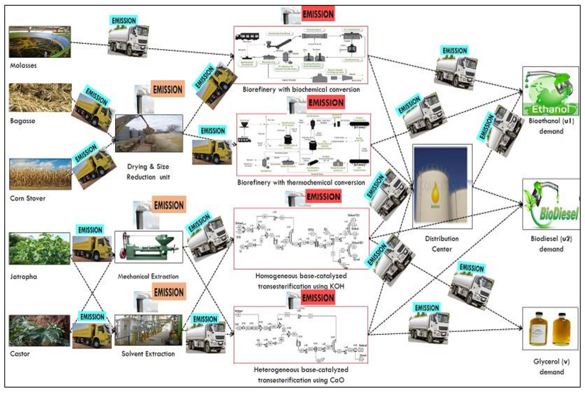
• Biomass preprocessing

  a.1.

  Drying and size reduction

  At this prior stage of the life cycle, the corn stover and bagasse are subjected to solar drying to drop down their moisture content from 20% [26] and 50% (average moisture content of bagasse produced in Ethiopia sugar industries), respectively, to 10%. Thereafter, the sizes of the feedstocks are reduced using a hammer mill, operated at a speed of 2000 rpm for 2 mm mesh size screen with 90° hammers. The research by Bitra et al. [27] and Kakolaki et al. [28] was used to compute the energy requirement of the mill to process the corn stover and bagasse, respectively. Table 1 presents the mass flow of input and output components and energy requirements to process 1 ton of both lignocellulostic feedstocks through drying and a size reduction mechanism.

  a.2.

  Mechanical and solvent extraction

  At this stage, the jatropha and castor seeds collected from the respective supply sources are converted to their respective oils either via mechanical extraction or solvent extraction technologies. The inventory data of the two extraction technologies are computed based on the previous research of Cheng et al. [29], Hou et al. [30] and Kebede [31]. Table 2 provides the mass flow of input and output components and energy requirement to process 1 ton of both non-edible feedstocks, i.e., jatropha and castor seeds, through mechanical and solvent extraction technologies. The required amount of raw materials to process 1 ton of jatropha and castor is assumed to be similar [30] despite the amount of products and byproducts being different depending on the conversion rate of the oil from the two feedstocks.

• Biofuel production

  b.1.

  Biochemical and thermochemical conversion

  The bioethanol production from corn stover/sugarcane molasses/bagasse is conducted by using biochemical or thermochemical conversions. The inventory data for both technologies are estimated based on Aspen plus process models of Foust et al. [32] and Mu et al. [33], as well as a similar molasses-based bioethanol plant in Ethiopia. Table 3 presents the inventory data associated with input and output materials, energy used as well as waste generation to process 1 ton of molasses/corn stover/bagasse using both conversion technologies.

  b.2.

  Homogeneous and heterogeneous based catalyzed transesterification

  After oil extraction, the transesterification step is carried out to yield biodiesel from the jatropha/castor oil. The two technologies considered at this stage are homogeneous and heterogeneous transesterification. The inventory data for both transesterification technologies are obtained from Aspen plus process models of Tasić et al. [34], Kaewcharoensombat et al. [35], and other referenced previous works [30,31,36]. Here, an assumption is taken that the input and output materials and energy for transesterification of jatropha and castor oil is similar since the conversion rate of both oils to biodiesel through both technologies is almost similar. Table 4 presents the inventory data associated with input and output materials, energy used as well as waste generation to process 1 ton of jatropha/castor oil using both homogeneous and heterogeneous transesterification processes.

• Biomass, preprocessed biomass and biofuel transportation

Diesel-powered heavy trucks are used for transporting materials in all BBSC stages. Considering the widely used type of vehicles for material transportation in the case study area, Euro II trailer truck and Euro III tanker truck are assumed to transport the solid and liquid materials available in the BBSC, respectively.

iii.

Impact analysis

In this work, the ecocosts method is used to quantify the impacts of all the activities of the BBSC on the environment. This method was acquainted by Vogtlander and Bijma [37] and was amended three times, in 2007, 2012, and 2017. Ecocosts are costs the that indicate the environmental stress a product brings in accordance with the prevention of the stress throughout the life cycle of the product.

Table 1. Material and energy inputs and outputs in drying and size reduction in raw corn stover and bagasse.

Drying and Size Reduction
Inventory	Corn Stover Based	Bagasse Based
Input
Biomass (tons)	1.0	1.0
Energy consumption (KWh)	9.33 × 104	2.64 × 104
Output
Biomass (tons)	0.9	0.6
Water (tons)	0.1	0.4

Source: Own computation.

Table 1. Material and energy inputs and outputs in drying and size reduction in raw corn stover and bagasse.

Drying and Size Reduction
Inventory	Corn Stover Based	Bagasse Based
Input
Biomass (tons)	1.0	1.0
Energy consumption (KWh)	9.33 × 104	2.64 × 104
Output
Biomass (tons)	0.9	0.6
Water (tons)	0.1	0.4

Source: Own computation.

Table 2. Material and energy inputs and outputs in mechanical and solvent extraction of jatropha and castor seed.

Mechanical Extraction			Solvent Extraction
Inventory	Jatropha Based	Castor Based	Inventory	Jatropha Based	Castor Based
Input			Input
Seed (tons)	1.0	1.0	Seed (tons)	1.0	1.0
Water (liter)	70.00	70.00	Hexane (tons)	0.9	0.9
H3PO4 (kg)	0.33	0.33	Water (liter)	100.00	100.00
Steam (ton)	10.00	10.00	H3PO4 (kg)	0.72	0.72
Electricity (kWh)	6220.00	6220.00	Steam (ton)	1820.00	1820.00
			Electricity (kWh)	1020.00	1020.00
Output			Output
Oil (tons)	0.25	0.38	Oil (tons)	0.32	0.49
Meal (tons)	0.7	0.51	Meal (tons)	0.61	0.40
Sludge (kg)	17.00	25.84	Sludge (kg)	66.38	70.65
Water (liter)	92.37	140.40	Water (liter)	60.00	91.88
H3PO4 (aq) (kg)	7.96	12.10	Hexane (tons)	0.90	0.90
Solid waste (kg)	3.00	4.56	H3PO4 (aq) (kg)	7.74	11.85
			Solid waste (including hulls) (kg)	36.00	37.59

Source: Own computation.

Table 2. Material and energy inputs and outputs in mechanical and solvent extraction of jatropha and castor seed.

Mechanical Extraction			Solvent Extraction
Inventory	Jatropha Based	Castor Based	Inventory	Jatropha Based	Castor Based
Input			Input
Seed (tons)	1.0	1.0	Seed (tons)	1.0	1.0
Water (liter)	70.00	70.00	Hexane (tons)	0.9	0.9
H3PO4 (kg)	0.33	0.33	Water (liter)	100.00	100.00
Steam (ton)	10.00	10.00	H3PO4 (kg)	0.72	0.72
Electricity (kWh)	6220.00	6220.00	Steam (ton)	1820.00	1820.00
			Electricity (kWh)	1020.00	1020.00
Output			Output
Oil (tons)	0.25	0.38	Oil (tons)	0.32	0.49
Meal (tons)	0.7	0.51	Meal (tons)	0.61	0.40
Sludge (kg)	17.00	25.84	Sludge (kg)	66.38	70.65
Water (liter)	92.37	140.40	Water (liter)	60.00	91.88
H3PO4 (aq) (kg)	7.96	12.10	Hexane (tons)	0.90	0.90
Solid waste (kg)	3.00	4.56	H3PO4 (aq) (kg)	7.74	11.85
			Solid waste (including hulls) (kg)	36.00	37.59

Source: Own computation.

Table 3. Material and energy inputs and outputs in biochemical and thermochemical conversions of molasses/corn stover/bagasse.

Biochemical Conversion				Thermochemical Conversion
Inventory	Corn Stover Based	Molasses Based	Bagasse Based	Inventory	Corn Stover Based	Bagasse Based
Input				Input
Biomass (ton)	1.00	1.00	1.00	Biomass (ton)	1.00	1.00
Water consumption (liter)	1870.00	3580.00	760.00	Water consumption (liter)	540.00	320.00
Enzyme (kg)	9.08	4.12	3.65	Air (m3)	2953.78	1593.63
Yeast (kg)	2.26	3.41	2.26	MgO (kg)	0.18	0.02
Lime (kg)	22.48	12.97	14.37	Bed materials (kg)	2.30	1.35
Sulfuric acid (kg)	29.44	10.62	19.73	Synthesis catalyst (kg)	0.01	0.01
Corn steep liquor (kg)	11.19		7.73	Tar reforming catalyst (kg)	0.01	0.01
Diammonium phosphate (kg)	1.18	0.28	0.91	Oxidizer for S recovery (kg)	1.35	0.71
Sodium hydroxide (kg)	10.01	7.32	10.01
Urea (kg)	1.77	1.02	1.77
Output				Output
Bioethanol (ton)	0.23	0.26	0.27	Bioethanol (ton)	0.20	0.19
Carbon dioxide (ton)	0.87	0.24	0.67	Carbon dioxide (ton)	0.91	0.63
Electricity output (KWh)	701.03	307.21	701.03	Mixed alcohol (kg)	39.02	23.93
Vinasse (kg)	29.90	28.62	29.90	Sulfur (solid) (kg)	0.56	0.29
				Sand and ash (kg)	73.88	7.69

Source: Own computation.

Table 3. Material and energy inputs and outputs in biochemical and thermochemical conversions of molasses/corn stover/bagasse.

Biochemical Conversion				Thermochemical Conversion
Inventory	Corn Stover Based	Molasses Based	Bagasse Based	Inventory	Corn Stover Based	Bagasse Based
Input				Input
Biomass (ton)	1.00	1.00	1.00	Biomass (ton)	1.00	1.00
Water consumption (liter)	1870.00	3580.00	760.00	Water consumption (liter)	540.00	320.00
Enzyme (kg)	9.08	4.12	3.65	Air (m3)	2953.78	1593.63
Yeast (kg)	2.26	3.41	2.26	MgO (kg)	0.18	0.02
Lime (kg)	22.48	12.97	14.37	Bed materials (kg)	2.30	1.35
Sulfuric acid (kg)	29.44	10.62	19.73	Synthesis catalyst (kg)	0.01	0.01
Corn steep liquor (kg)	11.19		7.73	Tar reforming catalyst (kg)	0.01	0.01
Diammonium phosphate (kg)	1.18	0.28	0.91	Oxidizer for S recovery (kg)	1.35	0.71
Sodium hydroxide (kg)	10.01	7.32	10.01
Urea (kg)	1.77	1.02	1.77
Output				Output
Bioethanol (ton)	0.23	0.26	0.27	Bioethanol (ton)	0.20	0.19
Carbon dioxide (ton)	0.87	0.24	0.67	Carbon dioxide (ton)	0.91	0.63
Electricity output (KWh)	701.03	307.21	701.03	Mixed alcohol (kg)	39.02	23.93
Vinasse (kg)	29.90	28.62	29.90	Sulfur (solid) (kg)	0.56	0.29
				Sand and ash (kg)	73.88	7.69

Source: Own computation.

Table 4. Material and energy inputs and outputs in homogeneous and heterogeneous transesterification of jatropha/castor oil.

Homogeneous Transesterification		Heterogeneous Transesterification
Inventory	Jatropha/Castor Oil Based	Inventory	Jatropha/Castor Oil Based
Input		Input
Oil (ton)	1.00	Oil (ton)	1.00
Methanol (kg)	68.00	Methanol (kg)	58.09
KOH (kg)	10.00	CaO (kg)	50.48
H3PO4 (kg)	5.84	Electricity (KWh)	308.47
Water (liter)	138.53
Electricity (KWh)	779.79
Output		Output
Biodiesel (ton)	0.95	Biodiesel (ton)	0.96
Glycerol (kg)	89.00	Glycerol (kg)	98.00
Unreacted oil (kg)	33.05	CaO (kg)	50.48
Water with waste methanol (liter)	137.60
Solid residues (K3PO4) (kg)	12.72

Source: Own computation.

Table 4. Material and energy inputs and outputs in homogeneous and heterogeneous transesterification of jatropha/castor oil.

Homogeneous Transesterification		Heterogeneous Transesterification
Inventory	Jatropha/Castor Oil Based	Inventory	Jatropha/Castor Oil Based
Input		Input
Oil (ton)	1.00	Oil (ton)	1.00
Methanol (kg)	68.00	Methanol (kg)	58.09
KOH (kg)	10.00	CaO (kg)	50.48
H3PO4 (kg)	5.84	Electricity (KWh)	308.47
Water (liter)	138.53
Electricity (KWh)	779.79
Output		Output
Biodiesel (ton)	0.95	Biodiesel (ton)	0.96
Glycerol (kg)	89.00	Glycerol (kg)	98.00
Unreacted oil (kg)	33.05	CaO (kg)	50.48
Water with waste methanol (liter)	137.60
Solid residues (K3PO4) (kg)	12.72

Source: Own computation.

The ecocosts method was developed on the basis of the marginal prevention costs required to halt the negative impact of toxic emissions. These emissions are associated with human health as well as ecosystems, emissions that cause global warming, and resource depletion (metals, rare earths, fossil fuels, water, and land use). The concept of ecocosts is described in detail at http://www.ecocostsvalue.com/ (accessed on 10 February 2021) [38]. The ecocosts of a product are the sum of all ecocosts of global warming (CO₂ and other GHGs), human health, ecosystem, and natural resources depletion during its life cycle. The set of marginal prevention costs (multipliers) for the emissions of toxic substances used in the ecocosts 2017 system are as follows: An ecocost value of 8.75 EUR/kg SOx equivalent for acidification, 4.17 EUR/kg phosphate equivalent for eutrophication, 340.0 EUR/kg Cu equivalent for ecotoxicity, 3754 EUR/kg benzo(a)pyrene equivalent for human toxicity, 6.0 EUR/kg NOx equivalent for summer smog (respiratory diseases), 35.0 EUR/kg fine dust PM2.5 for fine dust, and 0.116 EUR/kg CO₂ equivalent for global warming (GWP 100).

In this work, the ecocosts method is selected due to the advantages it has comparing with other environmental indicators. Some of the advantages are (a) it is easy to understand and can be compared with economic criteria as it is given in monetary value; (b) comparison with another product is not mandatory unlike to other LCA methods; and (c) the system, including the costs, are updated every 5 years to incorporate the latest scientific advancements [38].

The emission and other utility consumption data acquired from the inventory analysis are placed at substance level, i.e., Consequently, the endpoint level impacts are calculated through the ecocosts method.

The minimization of total ecocosts of the entire BBSC is the environmental objective of this study. The total ecocost is given as the sum of the ecocosts of biomass preprocessing, biofuel production, and material transportation (Equation (8)). Ecocosts associated with processing raw and preprocessed biomasses available in the BBSC through their respective preprocessing and biorefinery technologies are given in

Table A1. Ecocosts associated with processing of raw and preprocessed biomass through the respective preprocessing and biorefinery technologies (USD/ton).

Process	Eco-Costs of GWP	Eco-Costs of Acidification	Eco-Costs of Eutrophication	Eco-Costs of Ecotoxicity (Freshwater)	Eco-Costs of Photochemical Oxidants	Eco-Costs of Fine Dust	Eco-Costs of Human Tocicity	Eco-Costs of Energy Carriers	Eco-Costs of Baseline Water Stress	Eco-Costs of Land-Use	Eco-Costs of Waste	Eco-Costs of Metals Scarcity	Eco-Costs of Carbon Footprint	Eco-Costs of Ecosystem	Eco-Costs of Human Health	Eco-Costs of ReSource Scarcity	Total Eco-Costs
Corn Stover Drying and Size Reduction	0.14	0.00	0.00	0.00	0.00	5.07	0.00	11.20	0.02	0.00	0.00	0.00	0.14	0.00	5.07	11.18	16.39
Corn Stover Biochemical Conversion	299.75	32.14	0.00	0.00	43.54	6.60	0.00	4.17	0.23	0.00	0.00	0.00	299.75	32.14	50.15	4.40	386.43
Corn Stover Thermochemical Conversion	408.49	12.11	0.00	0.00	17.18	2.13	0.00	10.20	0.29	0.00	0.00	0.00	408.49	12.11	19.31	10.49	450.41
Molasses Biochemical Conversion	271.48	3.72	3.20	0.00	6.88	0.89	0.00	3.34	0.20	0.00	0.00	0.00	271.48	6.92	7.77	3.54	289.72
Bagasse Drying and Size Reduction	0.01	0.00	0.00	0.00	0.00	3.05	0.00	8.06	0.02	0.00	0.00	0.00	0.01	0.00	3.05	8.05	11.11
Bagasse Biochemical Conversion	286.17	32.14	0.00	0.00	43.54	6.60	0.00	3.71	0.23	0.00	0.00	0.00	286.17	32.14	50.15	3.94	372.40
Bagasse Thermochemical Conversion	394.92	12.11	0.00	0.00	17.18	2.13	0.00	9.08	0.29	0.00	0.00	0.00	394.92	12.11	19.31	9.38	435.73
Jatropha Mechanical Extraction	53.46	1.48	0.00	0.00	1.88	1.17	0.00	195.01	0.00	0.00	0.00	0.00	53.46	1.48	3.05	195.01	253.01
Jatropha Solvent Extraction	7.80	0.22	0.00	0.00	0.27	0.17	0.00	26.65	0.00	0.00	0.00	0.00	7.80	0.22	0.45	26.65	35.12
Jatropha Homogeneous Transesterification	105.99	1.02	0.00	0.00	1.28	0.65	0.00	84.15	0.01	0.00	0.00	0.00	105.99	1.02	1.93	84.15	193.08
Jatropha Heterogeneous Transesterification	52.98	0.39	0.00	0.00	0.49	0.25	0.00	32.33	0.00	0.00	0.00	0.00	52.98	0.39	0.74	32.33	86.44
Castor Mechanical Extraction	53.46	1.48	0.00	0.00	1.88	1.17	0.00	195.01	0.00	0.00	0.00	0.00	53.46	1.48	3.05	195.01	253.01
Castor Solvent Extraction	7.80	0.22	0.00	0.00	0.27	0.17	0.00	26.65	0.00	0.00	0.00	0.00	7.80	0.22	0.45	26.65	35.12
Castor Homogeneous Transesterification	17.27	16.69	0.00	0.00	20.61	4.40	0.00	84.15	0.01	0.00	0.00	0.00	17.27	16.69	25.01	84.15	143.12
Castor Heterogeneous Transesterification	17.27	16.69	0.00	0.00	20.61	4.40	0.00	0.00	0.00	0.00	0.00	0.00	17.27	16.69	25.01	0.00	58.97

of Appendix B. Moreover,

Table A2. Ecocosts associated with transportation per vehicle type (USD km⁻¹ Vehicle⁻¹).

Vehicle Type	Eco-Cost
Euro II diesel engine (for solid materials transportation)	0.03636
Euro III diesel engine (for liquid materials transportation)	0.02997

of Appendix B presents the ecocosts associated with transportation per vehicle type used in this study.

$$\begin{array}{cc}Min EcoCost=& {\displaystyle {\displaystyle \sum }_y}[ {\displaystyle {\displaystyle \sum }_{b\in B}}{\displaystyle {\displaystyle \sum }_{d\in D}}{\displaystyle {\displaystyle \sum }_{i\in I}}{\displaystyle {\displaystyle \sum }_{f\in F}}{\displaystyle {\displaystyle \sum }_{t\in T}}\left(ecpb{f}_{b,f}\ast Wbi{f}_{b,d,i,f,y,t}\right)\hfill \\ & +{\displaystyle {\displaystyle \sum }_{d\in D}}{\displaystyle {\displaystyle \sum }_{u\in U}}{\displaystyle {\displaystyle \sum }_{j\in J}}{\displaystyle {\displaystyle \sum }_{g\in G}}{\displaystyle {\displaystyle \sum }_{t\in T}}\left(ecpd{g}_{d,g}\ast Wdj{g}_{d,u,j,g,y,t}\right) \hfill \\ & +{\displaystyle {\displaystyle \sum }_{b\in B}}{\displaystyle {\displaystyle \sum }_{h\in H}}{\displaystyle {\displaystyle \sum }_{i\in I}}{\displaystyle {\displaystyle \sum }_{t\in T}}\left(ect{b}_b\ast vca{p}_b\ast di{s}_{h,i}\ast Fbh{i}_{b,h,i,y,t}\right)\hfill \\ & +{\displaystyle {\displaystyle \sum }_{d\in D}}{\displaystyle {\displaystyle \sum }_{i\in I}}{\displaystyle {\displaystyle \sum }_{j\in J}}{\displaystyle {\displaystyle \sum }_{t\in T}}\left(ect{d}_d\ast vca{p}_d\ast di{s}_{i,j}\ast Fdi{j}_{d,i,j,y,t}\right)\hfill \\ & +{\displaystyle {\displaystyle \sum }_{u\in U}}{\displaystyle {\displaystyle \sum }_{j\in J}}{\displaystyle {\displaystyle \sum }_{k\in K}}{\displaystyle {\displaystyle \sum }_{t\in T}}\left(ect{u}_u\ast vca{p}_u\ast di{s}_{j,k}\ast Fuj{k}_{u,j,k,y,t}\right)\hfill \\ & +{\displaystyle {\displaystyle \sum }_{u\in U}}{\displaystyle {\displaystyle \sum }_{k\in K}}{\displaystyle {\displaystyle \sum }_{m\in M}}{\displaystyle {\displaystyle \sum }_{t\in T}}\left(ect{u}_u\ast vca{p}_u\ast di{s}_{k,m}\ast Fuk{m}_{u,k,m,y,t}\right)\hfill \\ & +{\displaystyle {\displaystyle \sum }_{u\in U}}{\displaystyle {\displaystyle \sum }_{j\in J}}{\displaystyle {\displaystyle \sum }_{m\in M}}{\displaystyle {\displaystyle \sum }_{t\in T}}\left(ect{u}_u\ast vca{p}_u\ast di{s}_{j,m}\ast Fuj{m}_{u,j,m,y,t}\right)\hfill \\ & +{\displaystyle {\displaystyle \sum }_{v\in V}}{\displaystyle {\displaystyle \sum }_{j\in J}}{\displaystyle {\displaystyle \sum }_{n\in N}}{\displaystyle {\displaystyle \sum }_{t\in T}}\left(ect{v}_v\ast vca{p}_v\ast di{s}_{j,n}\ast Fvj{n}_{v,j,n,y,t}\right)]\hfill \end{array}$$

(8)

where ecpbf_b,f, and ecpdg_d,g are total ecocosts to convert unit amount of biomass type b with technology f, and unit amount of preprocessed biomass type d with technology g, respectively (USD/ton). ectb_b, ectd_d, ectu_u, and ectv_v are total ecocosts to transport biomass b, preprocessed biomass d, biofuel u, and coproduct v for unit distance, respectively (USD km⁻¹vehicle⁻¹). vcap_b, vcap_d, vcap_u, and vcap_v are capacity of a vehicle to transport biomass b, preprocessed biomass d, biofuel u, and coproduct v, respectively (vehicle ton⁻¹). dis_a,b is distance between two locations a and b per vehicle (km veh⁻¹).

3.2. Case Study

The proposed integrated strategic-tactical and economic-environment optimization model is applied to Ethiopia’s real case to evaluate its effectiveness, and ultimately support the sustainable design and plan of the biofuel sector of the country. It is a planned over a 20-year horizon and each month is considered as a time period. Accordingly, there are 240 periods in the planning horizon.

Ethiopia’s suitable land, favorable climate, and abundant water availability have endowed the country with immense biomass resources. As a result, the government of Ethiopia emphasizes the utilization of the abundant biomass for biofuel development. Bioethanol production from sugarcane molasses as well as the production of biodiesel from jatropha curcas, castor crop, and palm trees are the main strategic direction of the government [2,39]. Moreover, hopes have been raised for the utilization of lignocellulostic feedstocks, such as corn stover and bagasse, for bioethanol production due to their huge abundance, cellulosic composition, and potential to decrease any perceived competition between food and energy production. In line with the Ethiopian government’s strategy, the type of biofuels considered in this case study are bioethanol and biodiesel. Moreover, sugar cane molasses, and two lignocellulosic biomasses, i.e., sugarcane bagasse and corn stover, are considered for bioethanol production. Additionally, the two non-edible oil plants, i.e., jatropha and castor seed, are considered as biodiesel feedstocks. The potential locations for purchasing the feedstocks were restricted to the zones that produces the biomasses. The zones are the second-level administrative subdivision of the country, which is below regions and above districts.

Drying and size reduction is the only preprocessing mechanism considered for the two lignocellulosic biomasses. However, for the molasses, no preprocessing mechanism was taken into account. Additionally, solvent and mechanical extractions are the technologies examined for preprocessing of jatropha and castor to produce their respective oils. Bioethanol is produced from sugar cane molasses, and the two lignocellulosic biomasses via two alternative biorefinery technologies, namely, thermochemical conversion through gasification and biochemical conversion with acid pre-treatment. Similarly, biodiesel is produced from jatropha and castor oils in the biorefineries through the emerging heterogeneous [40] and conventional homogeneous base-catalyzed transesterification technologies using CaO and KOH, respectively [40]. Crude glycerol, which is generated from biodiesel production, is taken as a co-product for this case study as it provides a significant economic benefit. The four biorefinery technologies were selected due to the nature of the feedstocks, environment and economic conditions [39], and the presence of adequate techno-economic data for evaluation. Six different capacity levels are considered for each of the three supply chain components, i.e., preprocessing facility, biorefinery, and distribution center. Moreover, all 58 zones of Ethiopia are considered as candidate locations for the three supply chain components. The considered demand locations for bioethanol and biodiesel are the capital cities of the nine regions and two city administrations of Ethiopia as the data to project the biofuel demand of the vehicle are available for these 11 cities only.

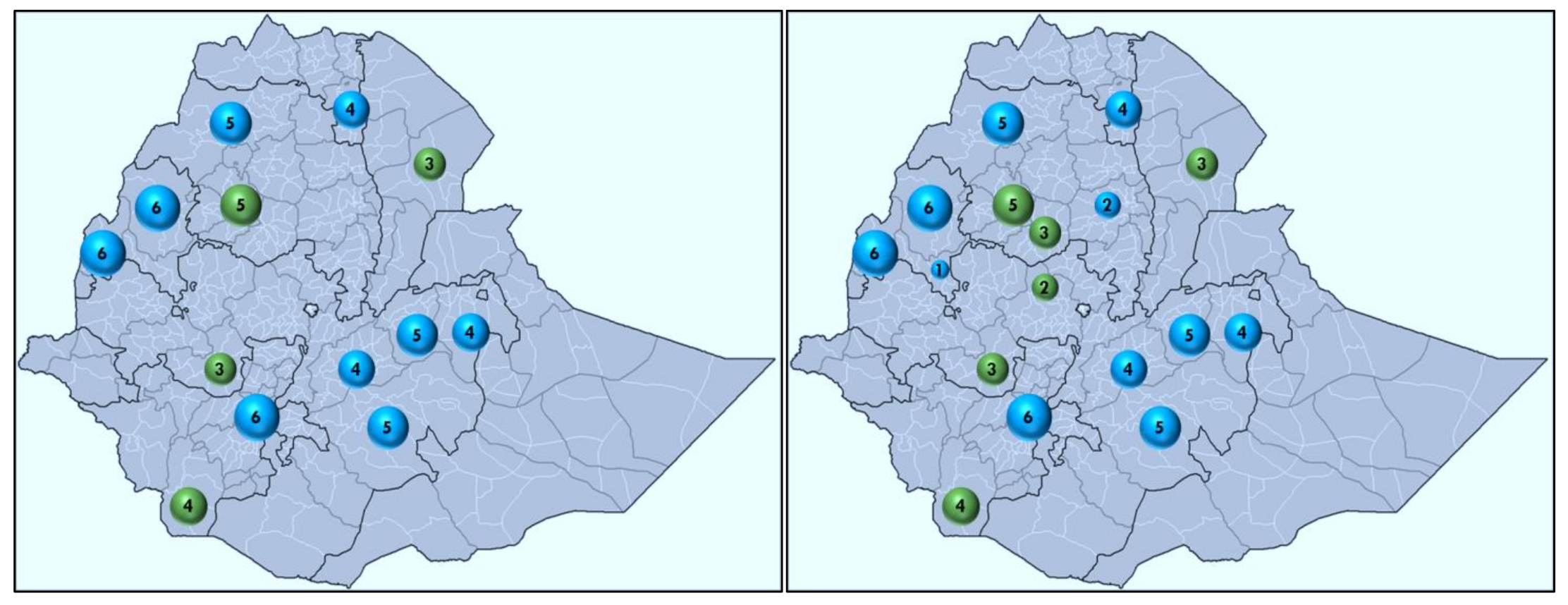
Despite the gathering of data being slightly challenging because it is a real, country-level case study, the authors attempted to the best of their ability to garner comprehensive, real data. Considering real data from responsible organizations in Ethiopia and data from the literature, the following assumptions were taken to estimate the technical, cost and environmental parameters of the BBSC.

• The annual production of molasses and bagasse is estimated based on the generation rate of the operational sugar factories in Ethiopia. Both the operational and under construction sugar factories, which are expected to start operation soon, are considered as potential suppliers of the two feedstocks. The amounts of molasses and bagasse were assumed to be zero in July and August as there was an experience of maintenance in the two months. The corn production data of each top corn producer zones in 2019/2020 [41] and corn stover-to-grain ratios [42] were used to estimate the stover generation amount. Since around 75% of the stover in Ethiopia is used as a cattle feed [43], the surplus 25% is considered. The land area (ha) dedicated to the cultivation of jatropha and castor in each zone [39,44,45] and their yield in terms of ton per ha (t.ha⁻¹) acquired from the current study of MoMPNG (Ministry of Mines, Petroleum and Natural Gas) [46] and FAO data [47] were used to estimate the amount of jatropha and castor seed produced.
• The quantity of bagasse, molasses and stover generation was assumed to be the same in each annum of the planning years. Contrarily, based on the projection from Ministry of Agriculture experts, the jatropha and castor quantity was considered to be double after 10 years. A potential variation from this assumption was addressed by conducting a sensitivity analysis on the biomass availability.
• Considering the status-quo of biofuel development in Ethiopia, government plan and type of vehicles available in the country, a forecast is made on bioethanol and biodiesel demand in the transportation sector. Consequently, in the years 2020/2021–2024/2025, 2025/2026–2029/2030, 2030/2031–2034/2035, and 2035/2036–2039/2040, a bioethanol blend with gasoline at 10%, 15%, 20%, and 25% by volume, respectively, was considered, whereas between the years 2020/2021–2029/2030, and 2030/2031–2039/2040, a biodiesel blend with diesel at 5% and 10% by volume, respectively, is assumed. A potential variation from the forecasted biofuels demand is addressed by conducting a sensitivity analysis. The Ethiopian Customs and Revenues Authority import data were used to forecast glycerol demand.
• The current purchasing prices of the biomasses and selling prices of the biofuels were considered in this study. The effect of potential variation from these prices on the results is addressed by conducting a sensitivity analysis.
• Based on the recommendation from Ethiopian Ministry of Economic Development and Cooperation to evaluate projects, a 10% discount rate was used in this case study.
• As there is shortage of real biorefinery and preprocessing plants in Ethiopia, most of the techno-economic data were predicted using previous research. Aspen Plus process models of Foust et al. [32] were used to determine the production and investment costs of the bioethanol producing biorefineries. Similarly, the investment and production costs of the two base-catalyzed transesterification technologies were estimated based on Aspen plus process models of Tasić et al. [34]. The cost of a similar plant built in Ethiopia was used to estimate the production cost associated with bioethanol production from molasses. The Lang Factor method [48] and data from Cao and Rosentrater [49] were used to predict the investment and production costs of the drying and size reduction unit, respectively. A material and energy balance was performed to estimate the production and investment costs of mechanical extraction. Then, the production and investment costs of solvent extraction was predicted based on a correlation from Cheng et al. [50]. Chemical engineering cost index values were used to actualize all cost data before 2019, which was taken as a reference year for all costs in the study. The investment and production costs for preprocessing and biorefineries with the six capacity levels were obtained using Chilton’s law equation [38].
• To transport all materials within the BBSC, the only road transportation mode was assumed by considering the case study area’s features. The road transportation distance between each zone was obtained from a geographic information system.
• Based on the current practice in Ethiopia, heavy-duty Euro II and Euro III diesel-engine vehicles were considered in this case study for transporting the solid (raw and preprocessed biomasses) and liquid (biofuels, co-product and preprocessed oils) materials along the BBSC, respectively. The transportation costs are estimated based on Ministry of Transport data.
• The production yields of preprocessing units and biorefineries via the different technologies were obtained from previous scientific studies and laboratory works.
• To ensure an adequate biomass supply, the storage capacity of the biorefinery and preprocessing units were assumed to accommodate the preprocessed and raw biomasses utilized for a year, respectively. This assumption is taken because of seasonal variation of feedstock availability, unsustainable corn cultivation habits, low-quality road infrastructure in some zones and recurrent interruption of sugar production in Ethiopia.
• Either outside atmosphere storage, covered structure, or enclosed structure was considered for storing each type of materials in the BBSC based on the condition (raw, pretreated or processed), phase and size of the material. The storage cost and monthly deterioration in each storage system were obtained from a previous scientific study [51].

The data used for all the technical and cost parameters of this case study are available in the Supplementary Materials.

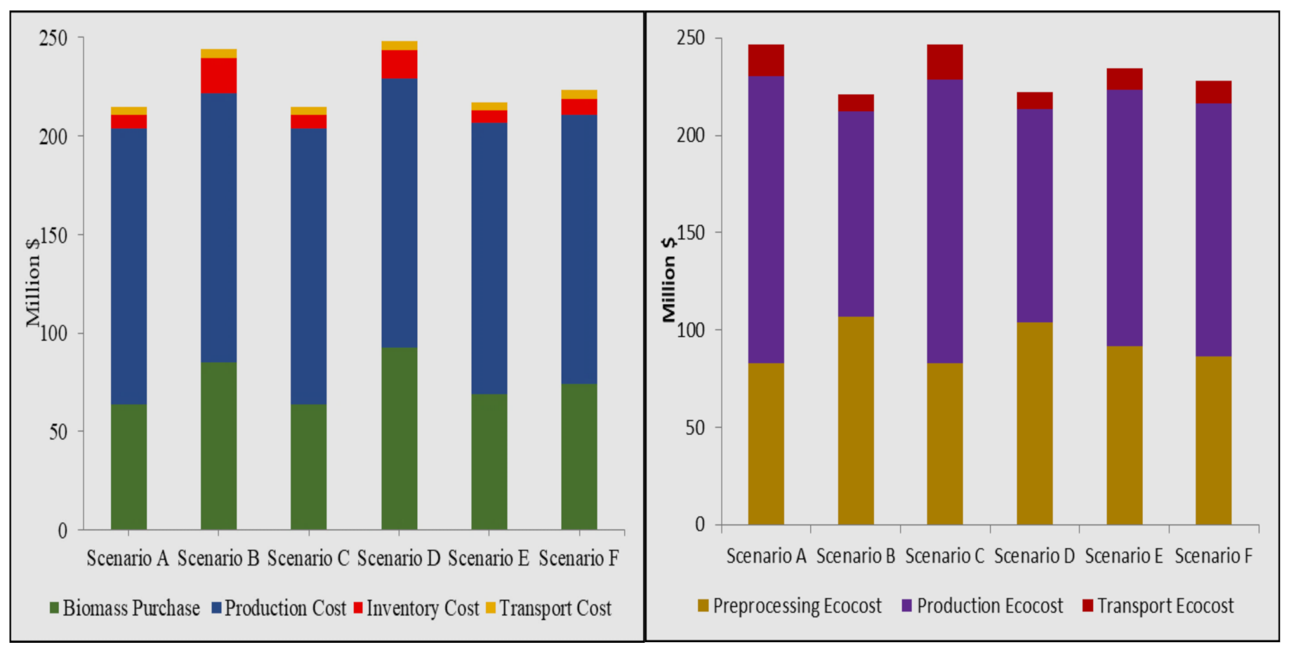
4. Results and Discussion

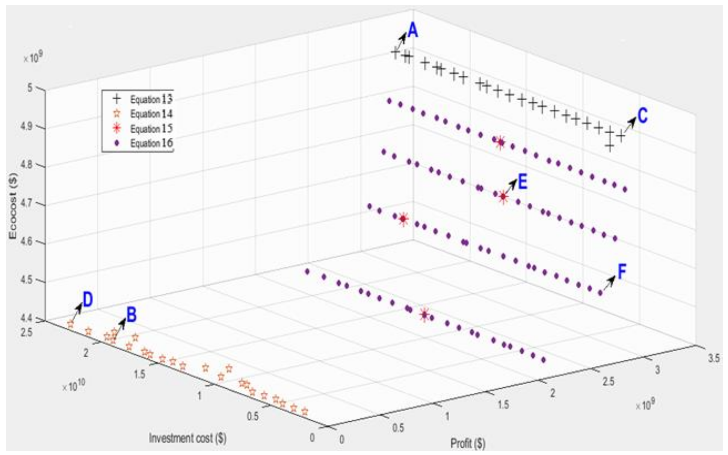
4.1. Multiobjective Optimization Strategy

Since this planning problem relies on three objective functions, it requires solution of a multi-objective MILP. The problem addressed in this study can be stated as follows.

$$\begin{array}{c}Objective function=\left\{\max profit,\min investment cost,\min ecocost\right\}\hfill \\ \mathrm{Subject} \mathrm{to} \mathrm{Constraints} \left(\mathrm{A}1\right)–\left(\mathrm{A}29\right)\hfill \end{array}$$

(9)

where profit, investment cost, and ecocost are defined in Equations (1), (7) and (8) respectively.

A series of mono-objective optimization problems were considered as presented in Equations (10)–(12) before solving the multi-objective problem.

$$\begin{array}{c}Objective function=\left\{\max profit\right\}\hfill \\ \mathrm{Subject} \mathrm{to} \mathrm{Constraints} \left(\mathrm{A}1\right)–\left(\mathrm{A}29\right)\hfill \end{array}$$

(10)

$$\begin{array}{c}Objective function=\left\{\min investment cost\right\}\hfill \\ \mathrm{Subject} \mathrm{to} \mathrm{Constraints} \left(\mathrm{A}1\right)–\left(\mathrm{A}29\right)\hfill \end{array}$$

(11)

$$\begin{array}{c}Objective function=\left\{\min ecocost\right\}\hfill \\ \mathrm{Subject} \mathrm{to} \mathrm{Constraints} \left(\mathrm{A}1\right)–\left(\mathrm{A}29\right)\hfill \end{array}$$

(12)

The mono-objective optimization models are solved using CPLEX 12.8 algorithm embedded in IBM ILOG. Then, the intention was to make a payoff table (see

Table 5. Payoff table.

Mono-Objective Optimization Case	Profit Value (M USD)	Investment Cost Value (M USD)	Ecocost Value (M USD)
Max profit Equation (10)	3110	22,081	4936
Min investment cost Equation (11)	-	-	-
Min ecocost Equation (12)	0.00	18,985	4416

) and acquire a balanced solution [38] that helps to seek an excellent compromise among the three antagonistic issues. Nevertheless, the attempt to solve Equation (11) (investment cost minimization) could not be successful, as the CPLEX ran out of memory. This is attributed to the sharp increment in model size, as it is a real countrywide case study with many continuous decision variables and parameters; in addition, it has many binary variables due to strategic choices, for example, the investment decisions related to location, capacity and technology of the BBSC components carried out on an annual basis.

Therefore, to obtain a good compromise between the profit and investment cost as well as ecocost and investment cost, the following procedures are used. We chose to solve Equations (10) and (12) with respect to different investment cost ranges, as specified in Equations (13) and (14) respectively.

$$\begin{array}{c}Objective function=\left\{\max profit\right\}\hfill \\ \mathrm{Subject} \mathrm{to} \mathrm{Constraints} \left(\mathrm{A}1\right)–\left(\mathrm{A}29\right)\hfill \\ Investment Cost{ }_{lower} \le Investment Cost \le Investment Cost{ }_{upper}\hfill \end{array}$$

(13)

$$\begin{array}{c}Objective function=\left\{\min ecocost\right\}\hfill \\ \mathrm{Subject} \mathrm{to} \mathrm{Constraints} \left(\mathrm{A}1\right)–\left(\mathrm{A}29\right)\hfill \\ Investment Cost{ }_{lower} \le Investment Cost \le Investment Cost{ }_{upper}\hfill \end{array}$$

(14)

As shown in Table 5, the range of the profit value between Equations (10) and (12) is very large, whereas the ecocost variation is not significant. Therefore, to obtain an additional set of feasible solutions that offers a good compromise between the profit and ecocost, Equation (10) is further solved with respect to different ecocost ranges as given in Equation (15). The ecocost values obtained in the profit maximization and ecocost minimization are taken as the upper and lower bounds, respectively.

$$\begin{array}{c}Objective function=\left\{\max profit\right\}\hfill \\ \mathrm{Subject} \mathrm{to} \mathrm{Constraints} \left(\mathrm{A}1\right)–\left(\mathrm{A}29\right)\hfill \\ Ecocost{ }_{lower} \le Ecocost \le Ecocost{ }_{upper}\hfill \end{array}$$

(15)

Moreover, to find a good compromise between the three objectives, Equations (13) and (15) are merged to offer the following equation:

$$\begin{array}{c}Objective function=\left\{\max profit\right\}\hfill \\ \mathrm{Subject} \mathrm{to} \mathrm{Constraints} \left(\mathrm{A}1\right)–\left(\mathrm{A}29\right)\hfill \\ Investment Cost{ }_{lower} \le Investment Cost \le Investment Cost{ }_{upper}\hfill \\ Ecocost{ }_{lower} \le Ecocost \le Ecocost{ }_{upper}\hfill \end{array}$$

(16)

Table 6. Statistics for Equations (13)–(16).

		Equation (13)	Equation (14)	Equation (15)	Equation (16)
Number of constraints		1,348,768	1,348,768	1,348,768	1,348,772
Number of binary variables		174	174	174	174
Number of continuous variables		2,404,430	2,404,430	2,404,430	2,404,430
CPU time using an Intel 2.60-GHz processor (minutes)	Min	32.49	29.05	58.42	157.21
	Max	176.01	169.45	102.42	668.58
Iterations	Min	3,079,950	2,989,417	3,258,726	4,484,996
	Max	6,332,344	6,051,353	5,187,132	25,247,564
Relative optimality gap (%)		0.01
Absolute optimality gap (%)		0.0001

provides the statistics for Equations (13)–(16). Moreover, the feasible solutions to the four equations are represented in Figure 3.

4.2. Optimum Solutions for Mono-Objectives

The most profitable and environmentally friendly solutions are represented by point A and B in Figure 3, which are labeled as Scenarios A and B in this paper, respectively.

Scenario A proposes molasses as the only feedstock for bioethanol production in the first 5 years, since it has lowest production cost. Then, to satisfy the required bioethanol production after 5 years, the utilization of corn stover is also recommended along with molasses due to its cheaper price. Regarding biodiesel feedstocks, both jatropha and castor are favored throughout the planning period. Scenario A involves the installation of fourteen biochemical and one thermochemical refinery for bioethanol and eighteen heterogeneous and one homogeneous catalysis transesterification refineries for biodiesel production between 2020/2021 and 2024/2025. Moreover, the required number of refineries increased between the periods 2025/2026–2029/2030, 2030/2031–2034/2035, and 2035/2036–2039/2040 by 21.42%, 28.57%, and 45.86% for biochemical; 200%, 600%, and 1700% for thermochemical; and 47.06%, 82.35%, and 117.6% for heterogeneous transesterification, respectively. To preprocess the raw feedstocks in the first five years of the planning period, one drying and size reduction as well as seven solvent and one mechanical extraction unit should be installed, in which numbers have shown a significant and consistent increment in the next 5–10, 11–15, and 16–20 years. Moreover, in the last 10 years of the planning period, Scenario A favors the building of a smaller number of mechanical extraction and homogeneous transesterification units with small capacities.

Despite Scenario B reducing the ecocost by 12% compared to Scenario A, it leads to almost zero profit. Similar to Scenario A, molasses is the only chosen feedstock to satisfy bioethanol production in the first 5 years. However, unlike to Scenario A, bagasse is the widely proposed bioethanol feedstock along with molasses after 5 years. This is attributed to relatively low fine particulate matter emissions associated with preprocessing of bagasse than corn stover. Similar to Scenario A, both jatropha and castor are recommended biodiesel feedstocks in all planning periods. In Scenario B, biochemical and heterogeneous transesterification refineries are exclusively chosen throughout the planning periods for bioethanol and biodiesel production, respectively, because of their lower GHG emission potential. Moreover, to reduce emissions, Scenario B recommends the installation of a smaller number of refineries comparing to Scenario A, but with higher capacities in fewer locations. In this scenario, the model proposes the installation of thirteen biochemical and fifteen heterogeneous transesterification refineries between 2020/2021 and 2024/2025. Moreover, the required number refineries increased by 6.25%, 18.75%, and 26.67% for the biochemical and by 46.67%, 86.67%, and 113.33% for heterogeneous transesterification between the periods 2025/2026–2029/2030, 2030/2031–2034/2035, and 2035/2036–2039/2040, respectively. In contrast to Scenario A, Scenario B favors the building of a greater number of preprocessing units with lower capacities in a location proximate to the feedstock supplies and distribution centers. This is mainly attributed to reduce transportation distance between biomass supply to preprocessing unit, and from biorefinery to demand zone, which ultimately reduces the vehicular emissions during biomass and biofuel transport.

4.3. Feasible Solutions for Bi-Objectives

The behavior of the graph for Equation (13) in Figure 3 has indicated that the extreme variation in the investment cost does not bring a significant change in the profit, i.e., the profit varies only by 0.42% when the investment cost increases from USD 3 to 22 billion. This indicates that deployment of number of biorefineries, preprocessing units, and distribution centers without designing optimum network of the BBSC is not a guarantee to obtain meaningful economic benefits. Nevertheless, the profit reduced significantly when the investment cost is downsized from USD 3 to 2 billion. The most feasible solution that corresponds to maximum profit but with a minimum investment cost is indicated by point C of Figure 4, which is labeled as Scenario C in this paper. In Scenario C, the model favors utilization of molasses and installation of biochemical refineries to produce bioethanol in the next 15 years. However, to satisfy the bioethanol demand in the next 16–20 years, corn stover should also be utilized and seven additional thermochemical refineries with their respective drying and size reduction units are required to be built. Regarding the biodiesel production, the model proposes the installation of heterogeneous transesterification refineries and solvent extraction units, in which their number has shown an increment with the planning period. Nevertheless, the installation of homogeneous transesterification refineries and mechanical extraction units is not supported in the entire planning year because of the higher production cost. Despite this, jatropha is chosen as the sole feedstock until 2024/2025; the usage of castor is proposed along with jatropha to attain the rising biodiesel demand after that year.

Similar to the profit maximization vs. investment cost variation, the behavior of the graph for Equation (14) in Figure 3 has indicated that the extreme increment in the investment cost does not bring a significant change in the ecocost. The reason is that the rise in investment cost is majorly associated with the deployment of more distribution centers, which does not have impact on ecocost due to the assumption that there is insignificant emission associated with storage of materials. Scenario D in this work implies the most feasible solution that corresponds to the lowest ecocost as well as lowest investment cost, and it is indicated by point D of Figure 3. In this Scenario, the model recommends an approximately similar network, biorefinery location and technology type to the one acquired in Scenario C. However, here, a greater number of preprocessing facilities with smaller capacities in few locations as well as more distribution centers are proposed. Moreover, no thermochemical based refineries are promoted, and bagasse is used as bioethanol feedstock in the last five planning years along with molasses compared with Scenario C.

The last bi-objective consideration is between the profit maximization and ecocost minimization. The antagonistic nature of the two objectives is assessed through the behavior of the graph for Equation (15) in Figure 3. Accordingly, the behavior has shown that a 2.5%, 5%, 7.5% and 10% reduction in the ecocost will decrease the profit by approximately 2%, 5.17%, 11% and 37%, respectively. Among the different solutions indicated in Figure 3, point E is the most feasible one to compromise the maximization of the profit and minimization of the ecocost and it is taken as Scenario E in this paper. The number, technology and capacity of biorefineries recommended in this scenario is almost similar to Scenario B, except there is very little variation in the number for the last five planning years. However, the numbers of preprocessing and distribution centers proposed in Scenario E are higher than the one recommended in Scenario A and significantly lower than Scenario B. Consequently, this scenario shows a small reduction in profit by 5% compared with Scenario A and a slight increment in the ecocost by 6% compared with Scenario B.

4.4. Feasible Solutions for Multi-Objectives

A set of efficient feasible solutions, which compromise the three objectives, is generated following the method described in Equation (16). In order to obtain a representative, feasible solution, the profit maximization forecast was run by taking four intervals for the ecocost and twenty-two intervals for the investment cost, generating a total of 88 feasible solutions (see the graph for Equation (16) in Figure 3). Among the feasible solutions, the one indicated as point F in Figure 4 is the best solution that compromises the three antagonistic objectives and labeled as Scenario F in this paper. In Scenario F, the model favors utilization of molasses in the first 10 planning years, which is then joined by both corn stover and bagasse to satisfy the bioethanol production in the next 11–20 years. Similar to the cases shown in most previous scenarios, Scenario F also recommends the utilization of both jatropha and castor for biodiesel production along the entire planning period. Moreover, the proposed preprocessing mechanisms for the lignocellulostic bioethanol feedstocks and biodiesel feedstocks are drying size reduction and solvent extraction, respectively. Biochemical and heterogeneous transesterification refineries are exclusively chosen throughout the planning periods for bioethanol and biodiesel production, respectively. In most cases, the refineries are proposed to be built in locations close to the biomass supply; despite this, a few are recommended to be located in high-biofuel-demand areas without biomass resources. The optimal strategic decisions (number, technology and capacity) of the preprocessing, and biorefinery for Scenario F for the different planning periods, are depicted in Figure 4 and Figure 5 respectively.

The average annual cost and ecocost components for the six scenarios are given in Figure 6. In all the six scenarios, the production cost constitutes the highest share of total cost by contributing 55 to 65% depending on the scenarios, followed by biomass purchase, inventory and transport cost. The highest biomass purchase cost is shown in the ecocost minimization scenarios (Scenario B and Scenario D), which is mainly attributed to the preference of bagasse as bioethanol feedstock than corn stover in these scenarios. Moreover, the highest inventory cost is also observed in these scenarios due to the installation of more preprocessing and distribution centers. The transport cost account for approximately 2% share of total cost in all scenarios.

The production and preprocessing stages cover more than 90% of the total ecocost, of which they account for 48–60%, and 34–49%, respectively, depending on the scenarios. Additionally, the remaining 3–7% of the total ecocost is covered by transportation of materials in the BBSC. The highest ecocost related to production is registered in Scenario A since it favors environmental unfriendly technologies, including homogeneous transesterification, thermochemical conversion and mechanical extraction, especially in the last planning periods. On the other hand, the maximum preprocessing ecocost is observed in Scenario B as the number of preprocessing facilities is higher. The transport ecocost is lowest in Scenario B and Scenario D, since they reduce transportation distance from biomass supply to preprocessing unit, and from biorefinery to demand zone is favored by selecting a higher number of preprocessing and distribution centers.

5. Conclusions and Perspectives

This study aims to design and plan a country-level biomass-to-biofuel supply chain (BBSC), taking into account economic-environmental perspectives, multiple time periods and a supply chain from field to product. To this end, a multi-period, multi-feedstock, multi-product, multi-echelon and multi-objective mixed-integer linear programming (MILP) model is developed. Compared to the other economic-environmental optimization models developed so far, the novelty of this model lies in the following issues: (1) The formulation of integrated model provides optimal strategic and tactical decisions simultaneously, rather than focusing on a conventional hierarchical approach, in which tactical decisions are made based on the optimal strategic decisions from the strategic-level model, and may arouse a non-optimal, sub-optimal and infeasible solutions. (2) The development of a comprehensive mathematical model of BBSC that intends to produce bioethanol and biodiesel simultaneously from five types of feedstocks and includes all the principal supply chain components, both upstream and downstream of the biorefineries.

The model is applied to Ethiopia’s actual case to offer a decision support tool for policymakers and other stakeholders, aiming to assist the development of the infant bioethanol and biodiesel sector in sustainable manner. A life cycle assessment was used to estimate the environmental impact along the BBSC and it is converted to monetary basis through ecocost approach. Since this planning problem relies on three objective functions—namely, profit, ecocost and investment costs—it requires a solution of a multi-objective MILP. However, the attempt to solve the latter with CPLEX could not succeed. This is due to the model size’s sharp increment, as it is an actual countrywide case study with many continuous decision variables and parameters, as well as availability of many binary variables due to strategic choices. Therefore, a new semi-heuristic approach, which offers a feasible solution to the problem, is provided to analyze the compromise between the objectives.

The results indicated that a clear tradeoff between the economic (profit) and environmental objectives. Accordingly, a 37% reduction in the profit is observed by decreasing the environmental burden (ecocost) of the BBSC by 10%. Moreover, further minimization of the ecocost by 12% leads to almost no profit. Contrarily, the variation in the investment cost does not have a significant impact on both profit and ecocost. The most feasible solution that compromise the three objectives has exclusively proposed the installation of biochemical and heterogeneous transesterification refineries for bioethanol and biodiesel production, respectively. Most of the refineries are located in areas close to the biomass supply locations rather than biofuel demand locations, whereas the opposite is true for a small number of refineries.

Numerous paths for the future expansion of this study are expected to be explored: (1) The incorporation of additional optimization objectives associated with other dimensions of sustainability, such as social, political, and technological dimensions. (2) The performance of either a very computationally demanding global sensitivity analysis or incorporate stochasticity in the model to address uncertainties in the input data (e.g., biomass availability, biomass purchase price, biofuel production costs and selling prices, and biofuel demand). (3) The exploration of solving methods for such large, national-level, multi-objective, and long-term planning problems to obtain optimal solutions, which is an upgraded version of the feasible solutions obtained in this study, with efficient resolution and acceptable computational time.

References

- FDRE. Ethiopia’s Climate-Resilient Green Economy (CRGE) Strategy. 2011. Available online: https://www.undp.org/content/dam/ethiopia/docs/Ethiopia%20CRGE.pdf (accessed on 29 May 2020).
- Negash, M.; Riera, O. Biodiesel value chain and access to energy in Ethiopia: Policies and business prospects. Renew. Sustain. Energy Rev. 2014, 39, 975–985. [Google Scholar] [CrossRef]
- Tesfamichael, B.; Montastruc, L.; Negny, S.; Yimam, A. Designing and planning of Ethiopia’s biomass-to-biofuel supply chain through integrated strategic-tactical optimization model considering economic dimension. Comput. Chem. Eng. 2021, 153, 107425. [Google Scholar] [CrossRef]
- Pérez, A.T.E.; Camargo, M.; Rincon, P.C.N.; Marchant, M.A. Key challenges and requirements for sustainable and industrialized biorefinery supply chain design and management: A bibliographic analysis. Renew. Sustain. Energy Rev. 2017, 69, 350–359. [Google Scholar] [CrossRef]
- Li, Q.; Hu, G. Supply chain design under uncertainty for advanced biofuel production based on bio-oil gasification. Energy 2014, 74, 576–584. [Google Scholar] [CrossRef] [Green Version]
- You, F.; Tao, L.; Graziano, D.J.; Snyder, S.W. Optimal design of sustainable cellulosic biofuel supply chains: Multiobjective optimization coupled with life cycle assessment and input-output analysis. AIChE J. 2012, 58, 1157–1180. [Google Scholar] [CrossRef] [Green Version]
- Cambero, C.; Sowlati, T.; Pavel, M. Economic and life cycle environmental optimization of forest-based biorefinery supply chains for bioenergy and biofuel production. Chem. Eng. Res. Des. 2016, 107, 218–235. [Google Scholar] [CrossRef]
- Murillo-Alvarado, P.E.; Guillén-Gosálbez, G.; Ponce-Ortega, J.M.; Castro-Montoya, A.J.; Serna-González, M.; Jiménez, L. Multi-objective optimization of the supply chain of biofuels from residues of the tequila industry in Mexico. J. Clean. Prod. 2015, 108, 422–441. [Google Scholar] [CrossRef]
- Santibañez-Aguilar, J.E.; González-Campos, B.; Ponce-Ortega, J.M.; Serna-González, M.; El-Halwagi, M. Optimal planning and site selection for distributed multiproduct biorefineries involving economic, environmental and social objectives. J. Clean. Prod. 2014, 65, 270–294. [Google Scholar] [CrossRef]
- Babazadeh, R.; Razmi, J.; Pishvaee, M.S.; Rabbani, M. A sustainable second-generation biodiesel supply chain network design problem under risk. Omega 2017, 66, 258–277. [Google Scholar] [CrossRef] [Green Version]
- Zore, Ž.; Čuček, L.; Kravanja, Z. Synthesis of sustainable production systems using an upgraded concept of sustainability profit and circularity. J. Clean. Prod. 2018, 201, 1138–1154. [Google Scholar] [CrossRef]
- Barbosa-Póvoa, A.P.; da Silva, C.; Carvalho, A. Opportunities and challenges in sustainable supply chain: An operations research perspective. Eur. J. Oper. Res. 2018, 268, 399–431. [Google Scholar] [CrossRef]
- Lam, H.L.; Varbanov, P.; Klemeš, J.J. Optimisation of regional energy supply chains utilising renewables: P-graph approach. Comput. Chem. Eng. 2010, 34, 782–792. [Google Scholar] [CrossRef]
- Čuček, L.; Martin, M.; Grossmann, I.E.; Kravanja, Z. Multi-period synthesis of optimally integrated biomass and bioenergy supply network. Comput. Chem. Eng. 2014, 66, 57–70. [Google Scholar] [CrossRef]
- Akhtari, S.; Sowlati, T.; Griess, V.C. Integrated strategic and tactical optimization of forest-based biomass supply chains to consider medium-term supply and demand variations. Appl. Energy 2018, 213, 626–638. [Google Scholar] [CrossRef]
- Vogel, T.; Almada-Lobo, B.; Almeder, C. Integrated versus hierarchical approach to aggregate production planning and master production scheduling. OR Spectr. 2017, 39, 193–229. [Google Scholar] [CrossRef]
- Paradis, G.; Lebel, L.; D’Amours, S.; Bouchard, M. On the risk of systematic drift under incoherent hierarchical forest management planning. Can. J. For. Res. 2013, 43, 480–492. [Google Scholar] [CrossRef]
- Lin, T.; Rodríguez, L.F.; Shastri, Y.N.; Hansen, A.C.; Ting, K. Integrated strategic and tactical biomass–biofuel supply chain optimization. Bioresour. Technol. 2014, 156, 256–266. [Google Scholar] [CrossRef] [PubMed]
- Zhang, J.; Osmani, A.; Awudu, I.; Gonela, V. An integrated optimization model for switchgrass-based bioethanol supply chain. Appl. Energy 2013, 102, 1205–1217. [Google Scholar] [CrossRef]
- Ekşioğlu, S.D.; Acharya, A.; Leightley, L.E.; Arora, S. Analyzing the design and management of biomass-to-biorefinery supply chain. Comput. Ind. Eng. 2009, 57, 1342–1352. [Google Scholar] [CrossRef]
- Russo, D.; Spreafico, C. TRIZ-Based Guidelines for Eco-Improvement. Sustainability 2020, 12, 3412. [Google Scholar] [CrossRef] [Green Version]
- International Organization for Standardization. ISO 14040, Environmental Management-Life Cycle Assessment-Principles and Framework (ISO 14040:2006); International Organization for Standardization: Geneva, Switzerland, 2006. [Google Scholar]
- Federal Transport Authority. Global Fuel Economy Initative, Final Draft Report on Pilot Global Fuel Economy Initiative Study in Ethiopia, Addis Ababa, 2012; Federal Transport Authority: Abu Dhabi, United Arab Emirates, 2012.
- Khoshnevisan, B.; Rafiee, S.; Tabatabaei, M.; Ghanavati, H.; Mohtasebi, S.S.; Rahimi, V.; Shafiei, M.; Angelidaki, I.; Karimi, K. Life cycle assessment of castor-based biorefinery: A well to wheel LCA. Int. J. Life Cycle Assess. 2018, 23, 1788–1805. [Google Scholar] [CrossRef]
- Soam, S.; Kumar, R.; Gupta, R.P.; Sharma, P.K.; Tuli, D.K.; Das, B. Life cycle assessment of fuel ethanol from sugarcane molasses in northern and western India and its impact on Indian biofuel programme. Energy 2015, 83, 307–315. [Google Scholar] [CrossRef]
- Tesfamichael, B.; Gessese, N. Effect of Biochar Application Rate, Production (Pyrolysis) Temperature and Feedstock Type (Rice Husk/Maize Straw) on Amendment of Clay-Acidic Soil. In Lecture Notes of the Institute for Computer Sciences, Social Informatics and Telecommunications Engineering; Springer: Berlin/Heidelberg, Germany, 2019; pp. 135–144. [Google Scholar]
- Bitra, V.S.; Womac, A.; Chevanan, N.; Miu, P.I.; Igathinathane, C.; Sokhansanj, S.; Smith, D.R. Direct mechanical energy measures of hammer mill comminution of switchgrass, wheat straw, and corn stover and analysis of their particle size distributions. Powder Technol. 2009, 193, 32–45. [Google Scholar] [CrossRef]
- Kinamehr, M.H.; Abooali, B. Influence of feed moisture and hammer mill operating factors on bagasse particle size distributions. Agric. Eng. Int. CIGR J. 2020, 22, 180–188. [Google Scholar]
- Cheng, M.-H.; Sekhon, J.J.; Rosentrater, K.A.; Wang, T.; Jung, S.; Johnson, L.A. Environmental impact assessment of soybean oil production: Extruding-expelling process, hexane extraction and aqueous extraction. Food Bioprod. Process. 2018, 108, 58–68. [Google Scholar] [CrossRef]
- Hou, J.; Zhang, P.; Yuan, X.; Zheng, Y. Life cycle assessment of biodiesel from soybean, jatropha and microalgae in China conditions. Renew. Sustain. Energy Rev. 2011, 15, 5081–5091. [Google Scholar] [CrossRef]
- Abebe, D.K. A Life Cycle Assessment on Liquid Biofuel Use in the Transport Sector of Ethiopia. Ph.D. Thesis, University of South Africa, Pretoria, South Africa, 2013. [Google Scholar]
- Foust, T.; Aden, A.; Dutta, A.; Phillips, S. An economic and environmental comparison of a biochemical and a thermochemical lignocellulosic ethanol conversion processes. Cellulose 2009, 16, 547–565. [Google Scholar] [CrossRef]
- Mu, D.; Seager, T.; Rao, P.S.; Zhao, F. Comparative Life Cycle Assessment of Lignocellulosic Ethanol Production: Biochemical Versus Thermochemical Conversion. Environ. Manag. 2010, 46, 565–578. [Google Scholar] [CrossRef]
- Tasić, M.B.; Stamenković, O.S.; Veljković, V.B. Cost analysis of simulated base-catalyzed biodiesel production processes. Energy Convers. Manag. 2014, 84, 405–413. [Google Scholar] [CrossRef]
- Kaewcharoensombat, U.; Prommetta, K.; Srinophakun, T. Life cycle assessment of biodiesel production from jatropha. J. Taiwan Inst. Chem. Eng. 2011, 42, 454–462. [Google Scholar] [CrossRef]
- Liang, S.; Xu, M.; Zhang, T. Life cycle assessment of biodiesel production in China. Bioresour. Technol. 2013, 129, 72–77. [Google Scholar] [CrossRef]
- Vogtlander, J.G.; Bijma, A. The ‘Virtual Pollution Prevention Costs ‘99’. Int. J. Life Cycle Assess. 2000, 5, 113–120. [Google Scholar] [CrossRef]
- Miret, C.; Chazara, P.; Montastruc, L.; Negny, S.; Domenech, S. Design of bioethanol green supply chain: Comparison between first and second generation biomass concerning economic, environmental and social criteria. Comput. Chem. Eng. 2016, 85, 16–35. [Google Scholar] [CrossRef] [Green Version]
- Berhanu, M.; Jabasingh, S.A.; Kifile, Z. Expanding sustenance in Ethiopia based on renewable energy resources – A comprehensive review. Renew. Sustain. Energy Rev. 2017, 75, 1035–1045. [Google Scholar] [CrossRef]
- Marinković, D.; Stanković, M.V.; Veličković, A.V.; Avramović, J.M.; Miladinović, M.R.; Stamenković, O.; Veljković, V.B.; Jovanović, D.M. Calcium oxide as a promising heterogeneous catalyst for biodiesel production: Current state and perspectives. Renew. Sustain. Energy Rev. 2016, 56, 1387–1408. [Google Scholar] [CrossRef]
- CSA. Agricultural Sample Survey 2019/20: Report on Area and Production Of Major Crops, I. 2020. Available online: https://www.statsethiopia.gov.et/ (accessed on 29 May 2020).
- Marvin, W.A.; Schmidt, L.D.; Benjaafar, S.; Tiffany, D.G.; Daoutidis, P. Economic Optimization of a Lignocellulosic Biomass-to-Ethanol Supply Chain. Chem. Eng. Sci. 2012, 67, 68–79. [Google Scholar] [CrossRef]
- FAO. Ethiopia: Report on Feed Inventory and Feed Balance; FAO: Rome, Italy, 2018. [Google Scholar]
- Lakew, H.; Shiferaw, Y. Rapid Assessment of Biofuels Development Status in Ethiopia and Proceedings of the National Workshop on Environmental Impact Assessment and Biofuels; MELCA Mahiber: Addis Ababa, Ethiopia, 2008. [Google Scholar]
- Salehu, F.; Abebe, S.; Walle, T. Implementing Biofuels Programme for Household and Transport Energy Use; Case Study On Regulatory Reforms for Adoption of Biofuels Programme in Ethiopia; MELCA Mahiber: Addis Ababa, Ethiopia, 2015. [Google Scholar]
- MoMPNG. Baseline, Suitability Map, and Value Chain Study on Biofuel Development of Ethiopia; MELCA Mahiber: Addis Ababa, Ethiopia, 2018. [Google Scholar]
- FAO. FAOSTAT. 2019. Available online: http://www.fao.org/faostat/en/#home (accessed on 26 December 2019).
- Peters, M.S.; Timmerhaus, K.D.; West, R.E. Plant Design and Economics for Chemical Engineers; McGraw-Hill: New York, NY, USA, 2003. [Google Scholar]
- Cao, X.; Rosentrater, K.A. LCA and TEA of Corn Stover Size Reduction. In Proceedings of the 2016 ASABE International Meeting, Orlando, FL, USA, 17–20 July 2016. [Google Scholar] [CrossRef] [Green Version]
- Cheng, M.-H.; Dien, B.S.; Singh, V. Economics of plant oil recovery: A review. Biocatal. Agric. Biotechnol. 2019, 18, 101056. [Google Scholar] [CrossRef]
- Yue, D.; Slivinsky, M.; Sumpter, J.; You, F. Sustainable Design and Operation of Cellulosic Bioelectricity Supply Chain Networks with Life Cycle Economic, Environmental, and Social Optimization. Ind. Eng. Chem. Res. 2014, 53, 4008–4029. [Google Scholar] [CrossRef]