Abstract
This paper uses computational fluid dynamics (CFD) to simulate flow field distribution inside an electrochemical descaling reactor in three dimensions. First, the reactor flow field was obtained by steady-state simulation, and the grid independence was verified. Then, the steady state of the flow field was judged to ensure the accuracy of the simulation results. Transient simulations were performed on the basis of steady-state simulations, and residence time distribution (RTD) curves were obtained by a pulse-tracing method. The effects of plate height and plate spacing on reactor hydraulic characteristics (flow state and backmixing) were investigated using RTD curves, and the results showed that increasing the plate height and decreasing the plate spacing could make the flow more similar to the plug flow and reduce the degree of backmixing in the reactor. The flow field details provided by CFD were used to analyze the reactor flow field and were further verified to obtain the distribution patterns of dead and short circuit zones. Meanwhile, information regarding pressure drops was extracted for different working conditions (490, 560, and 630 mm for pole plate height and 172.6, 129.45, and 103.56 mm for pole plate spacing), and the results showed that increasing the pole plate height and decreasing the pole plate spacing led to an increased drop in pressure. In this case, a larger pressure drop means higher energy consumption. However, increasing the pole plate height had a smaller effect on energy consumption than decreasing the pole plate spacing.
1. Introduction
The circulating cooling water is used primarily for cooling equipment, dust removal, and the cooling of shower products in the industry. This process consumes large quantities of water. According to some statistics [1], industrial water consumption in China in 2019 was 121.76 billion cubic meters, accounting for 20% of total water consumption. In terms of industrial water, industrial cooling water accounted for about 60–70% of total industrial water consumption. Due to the exchange and transfer of heat, a scale will gradually form on the surface of heat-exchange equipment after accumulation. This scale causes higher energy consumption and equipment corrosion and, in severe cases, it may even explode. Several studies have documented that a scale of 3 mm in thickness can cause 20% of extra energy consumption, while a 9 mm-thick scale can cause 60% of extra energy consumption [2]. Therefore, to ensure production safety and decrease the treatment of energy consumption, the descaling of heat-exchange equipment is essential. Until recently, the method of adding chemicals has been widely used due to its low treatment costs and efficient effects. However, problems such as environmental pollution and secondary treatment of effluent also make it difficult to satisfy the needs of an environmentally friendly society [3,4,5]. The electrochemical treatment technology has increasingly been favored by researchers for its clean, non-polluting, and low-energy consumption features [6,7,8].
At present, many scholars have examined the descaling mechanism of electrochemical technology and have worked to improve its descaling efficiency. In 2021, Guo et al. [9] points out that the current magnitude can directly affect the descaling efficiency of an electrochemical system. In addition, it has been shown that the removal efficiency of both hardness and alkalinity increases with the increasing current. In 2019, Luan et al. [10] designed multi-meshes coupled cathodes—which produce a self-synergy effect based on their unique multilayer structure—that significantly improved descaling efficiency and further reduced energy consumption. In 2011, David Hasson [11] designed a novel descaling system that was characterized by the fact that the cathode and anode of the system were separated by a cationic ion exchange membrane and equipped with a separate reactor, thus avoiding the problem of cathode descaling. Furthermore, it can significantly increase the precipitation rate of CaCO3, significantly reduce the required electrode area, and overcome the fact that the conventional equipment is limited by the current limit. All of the above studies have made great contributions to the progress of electrochemical treatment technology, in which they offer something new in terms of improvements to electrical parameters and the development of new equipment. However, there is not a great deal of focus on the hydraulic characteristics of equipment, including internal water flow state, backmixing, etc.
Many scholars have conducted theoretical studies on the flow phenomena of fluids by developing universal mathematical models to guide and enable the intensification of flow processes [12,13,14]. However, whenever fluid flow is involved, the structure of the reactor is also an important factor that affects hydraulic flow characteristics [15]. The hydraulic characteristics of equipment have significant effects on improvements in descaling efficiency, equipment optimization, etc. One of the main approaches to the study of reactor mixing performance and hydraulic properties is the theory of residence time distribution. This concept was first proposed in 1935 by MacMullin and Weber for application in analytical chemical reactors and developed into a more explicit form through Danckwerts and Levenspiel et al. [16,17,18].
At the same time, flow field analysis is also an important mean for the study of the hydraulic characteristics of a reactor. However, the complicated nature of fluid motion has made it almost impossible to examine the flow field characteristics simply by direct field measurements or laboratory experiments. However, since the introduction of CFD in 1970, it has been easy to obtain complete flow field characteristics. Therefore, this method has been widely used in a variety of continuous flow systems. In 2010, Ding et al. [19] conducted a three-dimensional CFD simulation of a biohydrogen reactor. The authors derived reactor parameters with both performance and economy by optimizing its impeller structural parameters and analyzing the flow patterns of different types and speeds of the impeller. In 2017, Das et al. [20] performed two-dimensional simulations of multiphase flow in modified up-flow anaerobic sludge blanket (MUASB) and up-flow anaerobic sludge blanket (UASB) reactors. In addition, the authors compared and analyzed their hydrodynamic characteristics. The results showed that the mixing performance of MUASB was superior. Moreover, in the MUASB reactor, the appropriate baffle length and angle were more conducive to the mixing of materials. In the field of reactor design, CFD is a relatively mature research method [21,22,23], but few studies have used CFD to study the hydraulic characteristics of electrochemical descaling reactors.
In this paper, the internal structure of an electrochemical reactor is taken as the influencing factor, and the CFD method is adopted to simulate an electrochemical reactor in three dimensions with different structures. In Section 2, the RTD theory and numerical simulation scheme are described. In Section 3, results of the residence time distribution (RTD) and the reactor internal flow fields are presented from simulations. Moreover, this section analyzes the influence of structural changes to the reactor hydraulic characteristics and provides the theoretical basis for the design of electrochemical reactors with good hydraulic characteristics. In Section 4, the findings of our study are summarized and the concluding remarks are presented.
2. Methods
2.1. Methods of RTD
In an actual industrial reactor, due to the uneven flow rate of the reaction material or the influence of internal components, the reactor exists in a trench flow, dead zone, etc. This leads the reactor outlet material to have a different residence time in the reactor. According to the probability theory, the residence time distribution density function can be used to quantitatively describe the residence time distribution of the material in the reactor. This function can be written as:
where is the tracer concentration at the outlet as a function of time.
Since the curve has the property of normalization, the expression is:
For the curve, the mathematical expectation of residence time distribution is the average residence time of the material in reactor [24]. The mean residence time is the average time elapsed from the entry of fluid microelements into the reactor to their exit, and can be expressed by the following equation:
Variance, also known as dispersion, measures the degree of deviation of a random variable from its mean and is defined as:
In order to standardize and eliminate the inconvenience caused by different time units, dimensionless time can be introduced. The expression is:
Dimensionless time is substituted into Equation (1), and the corresponding residence time distribution density is:
Dimensionless time is substituted into Equation (4), and the corresponding variance is:
Since there is always a certain degree of backmixing in the reactor, it is generally described using the residence time. However, the degree of backmixing in the reaction is difficult to measure practically [25,26,27]. In addition, there is not necessarily a definite correspondence between the residence time and the degree of backmixing. Therefore, a mathematical modeling approach is needed to quantitatively describe the relationship between backmixing and residence time distribution.
When the reactor backmixing is minimal, it can be described by the axial dispersion model. According to the closed vessel boundary conditions, this can be:
where Pe is the Peclet number, D is the axial dispersion coefficient, is the line speed, and is the characteristic length. When Pe is 0, there is no axial mixing in the plug-flow. In addition, Pe is infinity, which indicates maximum axial mixing in the mixing flow. The rest represents the presence of different degrees of mixing in the reactor. As can be seen from the above equation, as long as the E(θ)curve is measured, variance can be derived and the Pe can be obtained.
Moreover, regardless of the reactor’s form, an actual reactor can be simulated by a tanks-in-series model, where N is the model parameter with a mixing flow, N is 1, and a plug-flow at N is infinity, which can be expressed by as [17,28,29]:
It can be proved that:
Similarly, the model’s parameters, N, can be calculated from the curve.
2.2. Geometry and Mesh
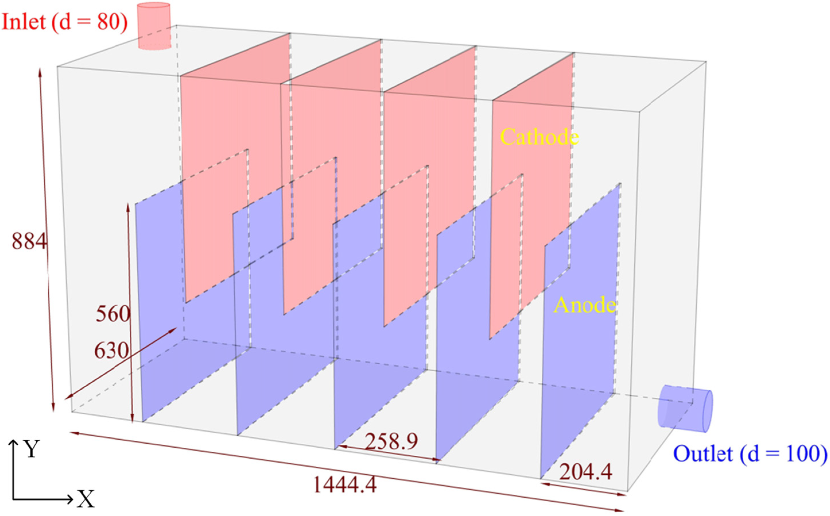
The physical model of the reactor was generated by the ANSYS Design Modeler [30] based on real reactor parameters at an equal scale. The reactor was equipped with an inlet (diameter was 80 mm) and an outlet (diameter was 100 mm), which were on the upper side and the right side of the reactor, respectively. The cathode and anode plates were alternately arranged inside the reactor. Their length, width, and height were 560, 4, and 630 mm, respectively. The distance between the anode plates (or cathode plates) was 258.9 mm and the length of the rightmost anode plate from the vessel wall was 204.4 mm. The raw water to be treated enters the reactor from the inlet. After an electrochemical reaction in the reactor, the water flows through the outlet to complete a cycle of descaling treatment. In order to save computational resources, some unnecessary details were simplified. The physical model is shown in Figure 1 after the modeling is completed, and all of the units in the figure are in millimeters (mm).

Figure 1.
Physical model diagram of electrochemical descaling reactor (all of the units are in mm).
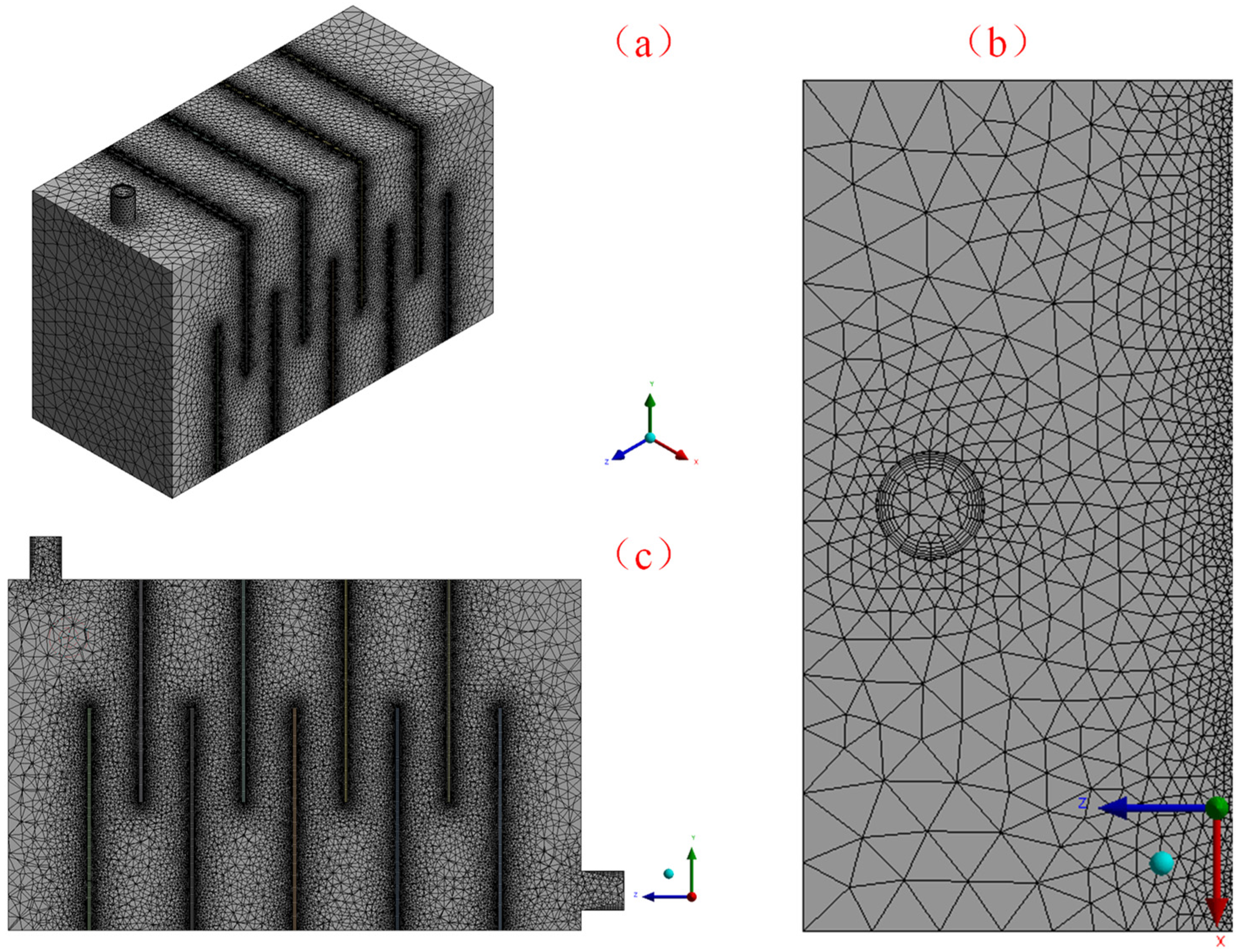
The fineness of the grid was an important factor affecting the calculation accuracy, calculation cost, and calculation speed. In this paper, the mesh was created in ANSYS Meshing [31]. Due to the friction between the fluid and the pipeline, there were large velocity gradients at the inlet and outlet. In addition, we set boundary layer meshes for the inlet and outlet to ensure the accuracy of the calculation results. Due to the large curvature at the inlet and outlet, and the narrow area in the model at the pole plate, we selected a smaller mesh size for these areas to improve the calculation accuracy. The other areas of the model were set with a larger mesh size to improve the computational speed and save costs. The completed grid is shown in Figure 2, and the total number of cells in the grid is 12302903. A combination of a tetrahedral grid and a hexahedral grid was used to divide the grid, and the average quality of the grid was above 0.81. The skewness was less than 0.2, which ensured the accuracy of the calculation results.
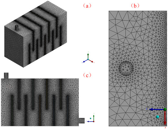
Figure 2.
Diagram of grid division in computational domain ((a): The 3D view of the grid; (b): The enlarged view of the grid at the inlet; (c): The YZ-plane cross-section of the grid at X = 315 mm).
2.3. Governing Equations
The objective of this paper is to examine the flow process of an incompressible Newtonian fluid in a reactor. As the energy loss and heat transfer due to the flow is small, we can assume that the temperature in the calculation domain is uniform [32,33]. In addition, the effect of gravity on the flow is neglected in this simulation due to the low reactor height. Therefore, the continuity equation and the momentum conservation equation can be used to describe this flow, as follows:
The concentration field of the tracer is obtained by solving the component transport equation to depict the RTD curve, which has the following general form:
Yi is the partial mass fraction of the ith component and Ji is the diffusion flux of components caused by concentration and temperature gradients. Since there is no diffusion caused by temperature gradients in this simulation, by the assumption of dilute approximation, the diffusion flux can be written as [32]:
is the diffusion coefficient for the ith species in the mixture.
2.4. Model Solution Procedure
Numerical simulations were performed by the pulse-tracer method in order to obtain the residence time distribution in two parts.
The first part was to solve the flow field of the steady-state calculation, and the simulation was based on the pressure solver. The flow model used the k-Ɛ two-equation turbulence model [34,35]. Here, the fluid material was defined as liquid water, the boundary condition of velocity inlet was used at the inlet, the inlet velocity was 2.60 m/s, and the turbulence was defined in terms of turbulence intensity and hydraulic diameter, which were 2.4% and 1.03 m, respectively. The boundary condition of the pressure outlet was used at the outlet, and its gauge pressure was set to 0. For the reactor wall, pole plate, and other components, the boundary condition of a standard no-slip wall was used. The second-order upwind discretization scheme was chosen for all of the equations in order to minimize numerical diffusions, and was solved with the coupled algorithm [36]. Physical parameters such as velocity and pressure were monitored in the calculation for an analysis later. In addition, we considered the calculation to have converged when the calculated residuals were less than 10−3.
The second part was the transient solution of the transport equation based on the convergent solution of the flow field of the steady-state calculation. Here, the physical properties of the tracer were set to be the same as water, the viscosity of the fluid mixture was set to 1 × 10⁻³ kg/(m·s), and the mass diffusivity was 1 × 10⁻⁹ m2/s. The inlet boundary condition was set to a mass fraction of 1 for the tracer and the pulse injection was completed within 0.50 s. Subsequently, the mass fraction of the tracer for the inlet boundary condition was set to 0. The RTD curve was obtained by setting a suitable maximum number of iterative and time steps to converge at each step and ensure that the residuals were reduced to between 10−4 and 10−7. Then, the tracer concentration was monitored at the outlet by area-weighted averaging.
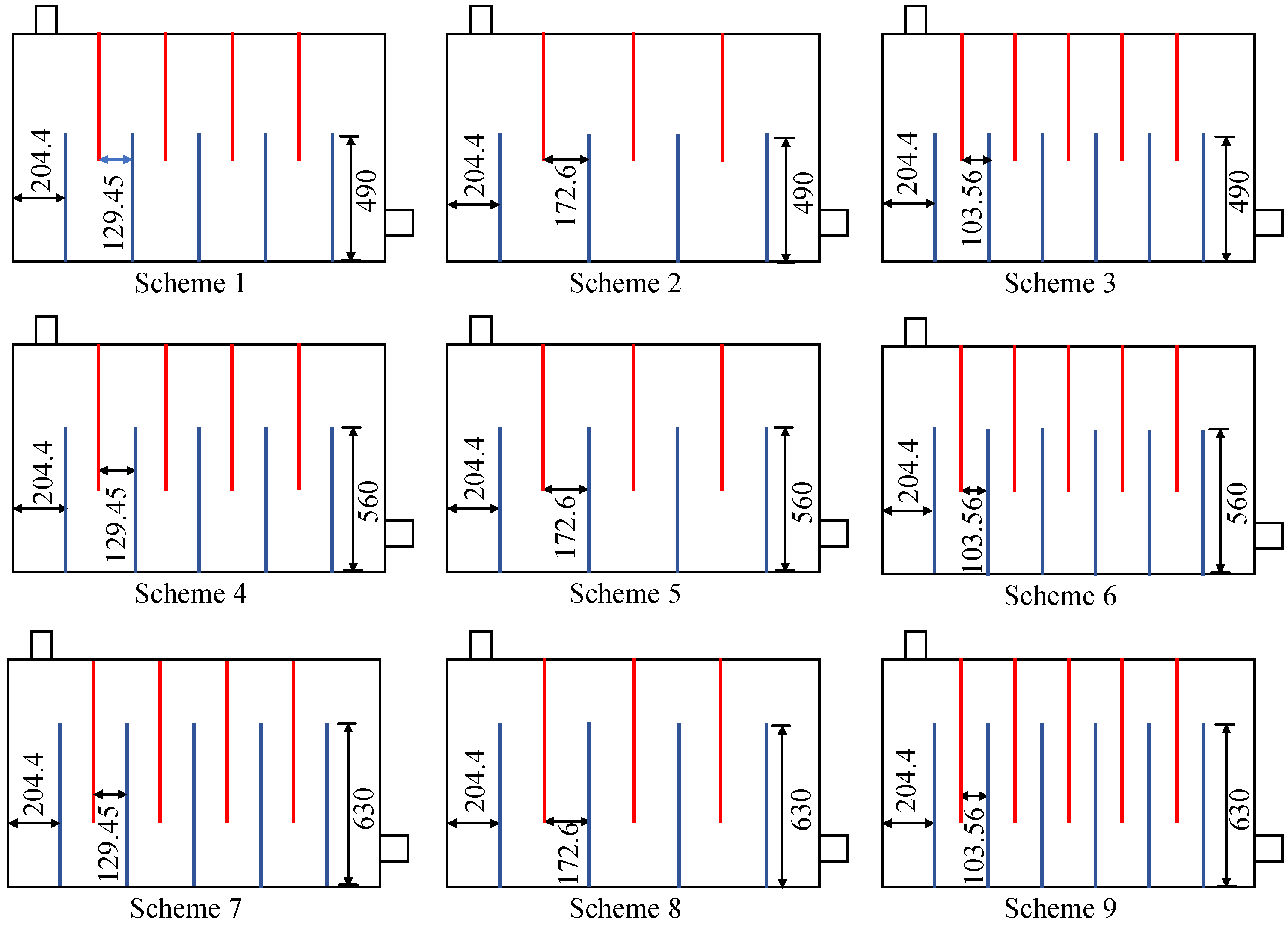
The boundary conditions used in the simulations are summarized in Table 1. Figure 3 is the schematic of the different tested configurations.

Table 1.
Summary of boundary conditions set in the simulation.
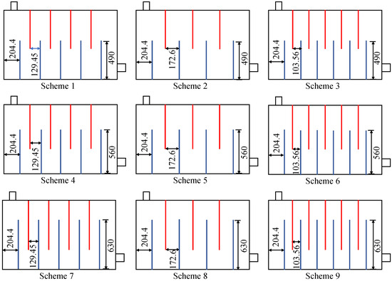
Figure 3.
Test configuration options (Scheme 1 is Ps = 129.45 and Pl = 490; Scheme 2 is Ps = 172.6 and Pl = 490; Scheme 3 is Ps = 103.56 and Pl = 490; Scheme 4 is Ps = 129.45 and Pl = 560; Scheme 5 is Ps = 172.6 and Pl = 560; Scheme 6 is Ps = 103.56 and Pl = 560; Scheme 7 is Ps = 129.45 and Pl = 630; Scheme 8 is Ps = 172.6 and Pl = 630; Scheme 9 is Ps = 103.56 and Pl = 630. All the above units are in mm).
3. Results and Discussion
3.1. Validation of Grid Independence
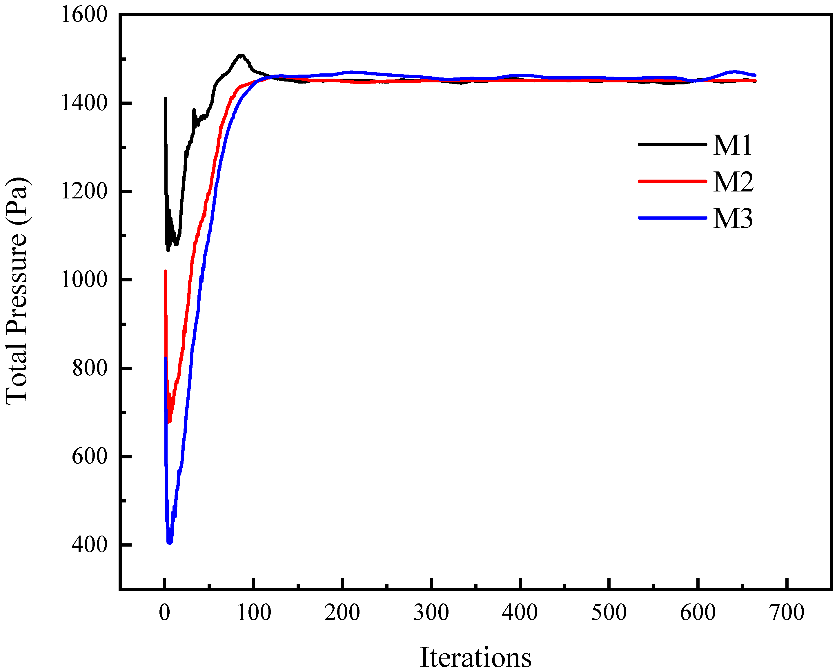
In order to eliminate the influence of grid size on the calculation results, the grid independence was verified for calculations with different numbers of grid cells (Ps = plate space = 129.45 mm; Pl = plate height = 560 mm). Simulations were performed using three different numbers of grids, i.e., M1 (10948191), M2 (5541889), and M3 (1776531), under the same operating conditions. In addition, the outlet velocity and total pressure were monitored by area-weighted averaging, respectively. The results are shown in Figure 4 and Table 2.
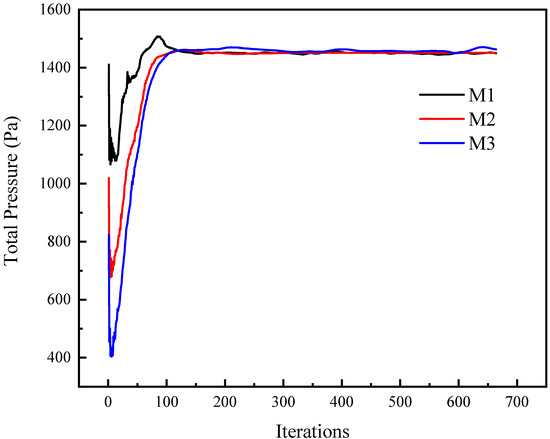
Figure 4.
Plot of total outlet pressure with iteration time (V = 2.6 m/s, Ps = 129.45 mm, Pl = 560 mm).
Table 2.
Validation results of grid independence.
As can be seen from Table 1, the trends in velocity and the total pressure at the reactor outlet do not change significantly with the increase in grid number. When the number of grids is encrypted from 5541889 to 10948191, it can be seen that the results no longer change. As can be seen from Figure 4, although the total outlet pressure shows a large difference in the initial stage, it is basically the same when the flow is stabilized. The computational errors of grids M1 and M2 for both the outlet velocity and total pressure were less than 1%, which indicated that the errors brought by the grid were acceptable for the experiment, and the M2 grid was finally used for the simulation.
3.2. Judgment of Flow Field Reaching the Steady State
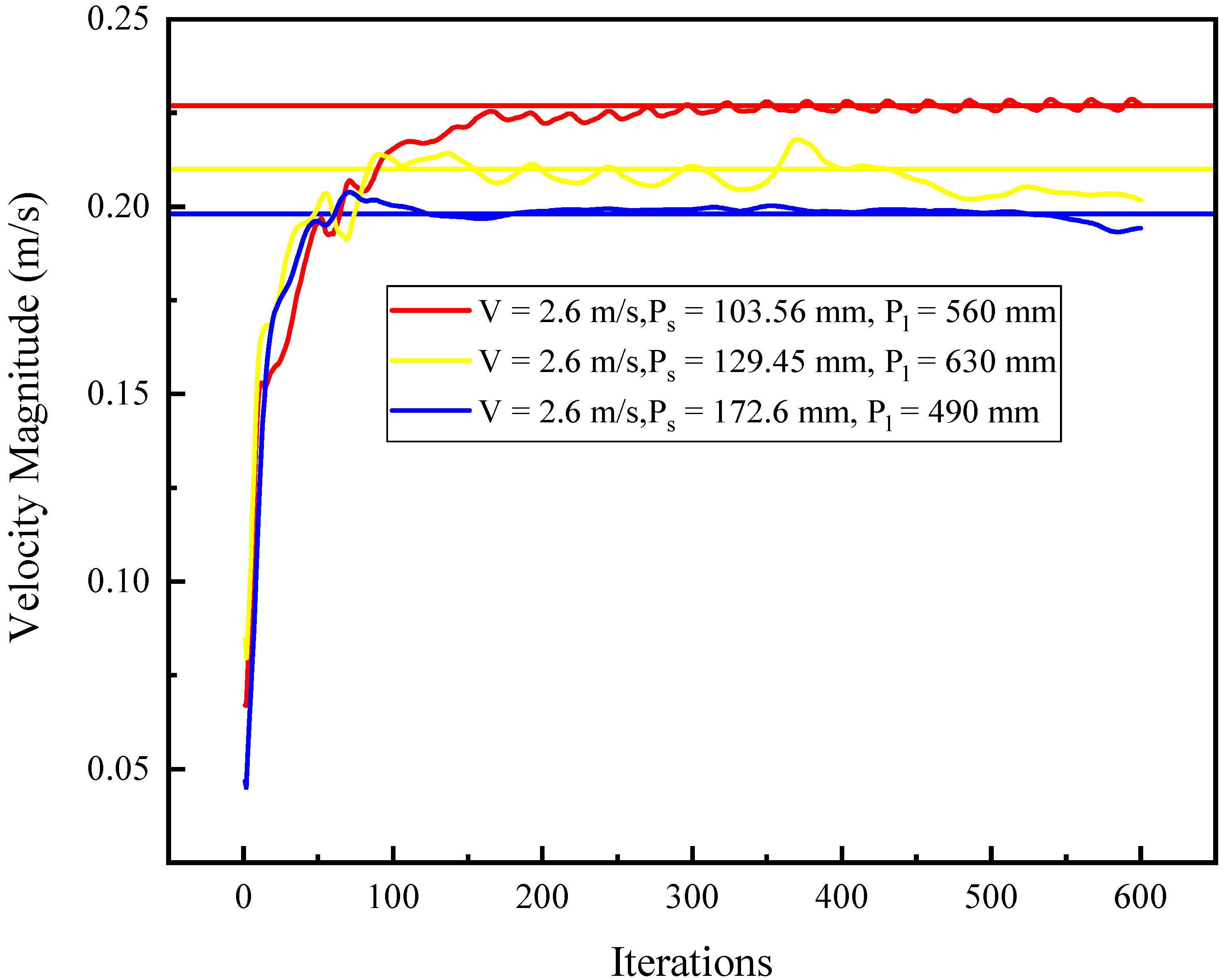
When obtaining the residence time distribution by a pulse-tracing method, we must note that the tracer can be injected into the reactor only when the flow field remains stable. Therefore, suitable evaluation criteria need to be proposed to determine the flow state of the flow field. Numerous studies have concluded that the flow field was considered to have reached a steady state when certain physical quantities in the fluid flow no longer fluctuated significantly [37,38,39]. Therefore, in this paper, the velocities in the reactor at three different operating conditions (V = 2.6 m/s, Ps = 103.56 mm, Pl = 560 mm; V = 2.6 m/s, Ps = 129.45 mm, Pl = 630 mm; and V = 2.6 m/s, Ps = 172.6 mm, Pl = 490 mm) were monitored by volume-weighted averaging to observe and determine that the flow field had stabilized. Figure 5 shows that, although their time to reach stability varies for each working condition, their average velocities in the reactor all reach a steady state: 0.227, 0.21, and 0.198 m/s, respectively. From this, we can assume that the flow field was at a steady state at each reaction condition when the tracer was pulse injected, and no errors or mistakes in RTD curves could be caused as a result.
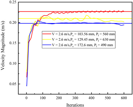
Figure 5.
Variations in speed with the number of iteration steps for each working condition.
3.3. The Effect of Plate Length on the Reactor’s Hydraulic Characteristics
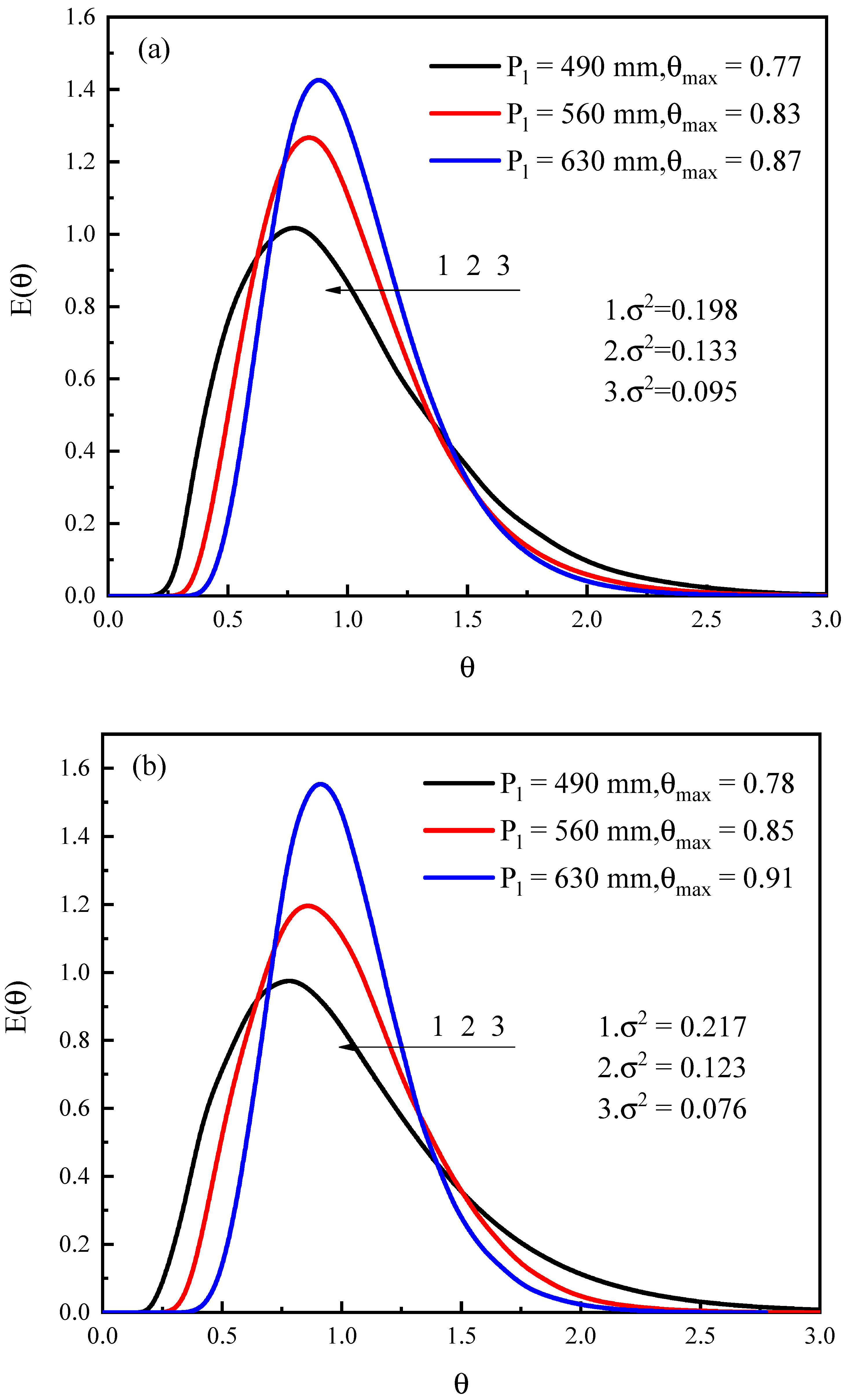
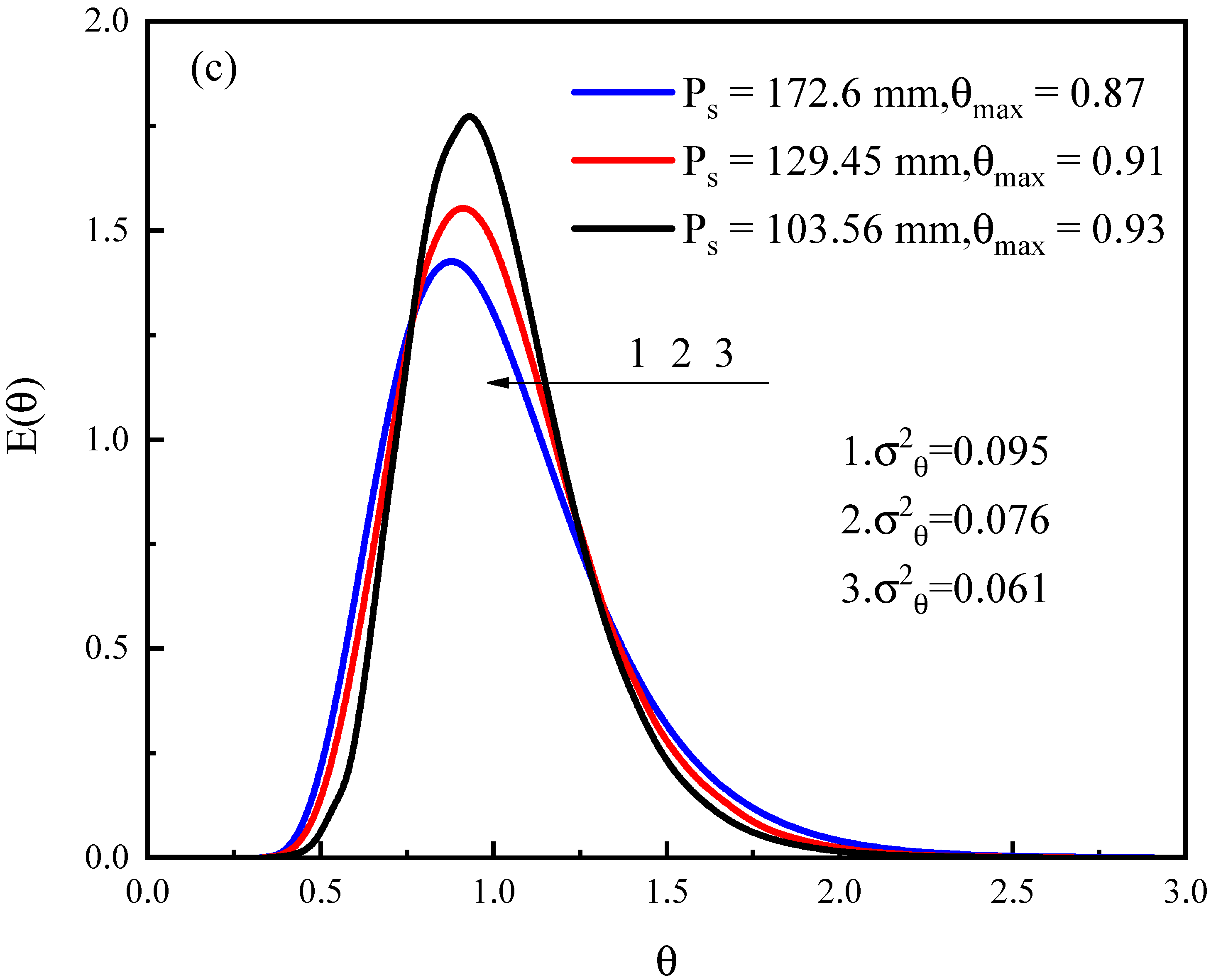
Figure 6 shows the variation in the RTD curve with the height of the pole plate for different plates. It is apparent from Figure 6 that the RTD curve has a more symmetrical distribution with the increase in plate height, which indicates a more uniform mixing of the fluid and less short-circuiting. Moreover, this was evidenced by the continuous increase in the maximum peak time, which was 0.77–0.87 (Ps = 172.6 mm), 0.78–0.91 (Ps = 129.45 mm), and 0.78-0.93 (Ps = 103.56 mm), with the increasing plate height at different plate spacings, respectively. The maximum peak time is 0.91, which indicates that the dead zone area and the degree of backmixing in the reactor are reduced. Furthermore, with the increase in plate height, we can observe that the tail of the RTD curve becomes shorter and the curve at the end is smoother. Many studies suggest that the longer the tail of the curve, the longer the dead zone formed in the reactor due to a slow flow rate or stagnant area. Therefore, from Figure 6, we can conclude that the increase in the height of the pole plate is beneficial to reduce the dead zone in the reactor. In addition, we found that the variance in RTD curves decreased with an increasing pole plate height at three different pole plate spacings, implying that the flow state of the reacting fluid was evolving towards the plug-flow.
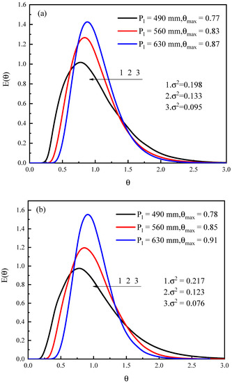

Figure 6.
Plot of the effect of pole plate height on the RTD curve ((a): The residence time distribution curves of the reactor when V is 2.6 m/s, Ps is 172.6 mm, and Pl is 490, 560 and 630 mm, respectively; (b): The residence time distribution curves of the reactor when V is 2.6 m/s, Ps is 129.45 mm, and Pl is 490, 560 and 630 mm, respectively; (c): The residence time distribution curves of the reactor when V is 2.6 m/s, Ps is 103.56 mm, and Pl is 490, 560 and 630 mm, respectively).
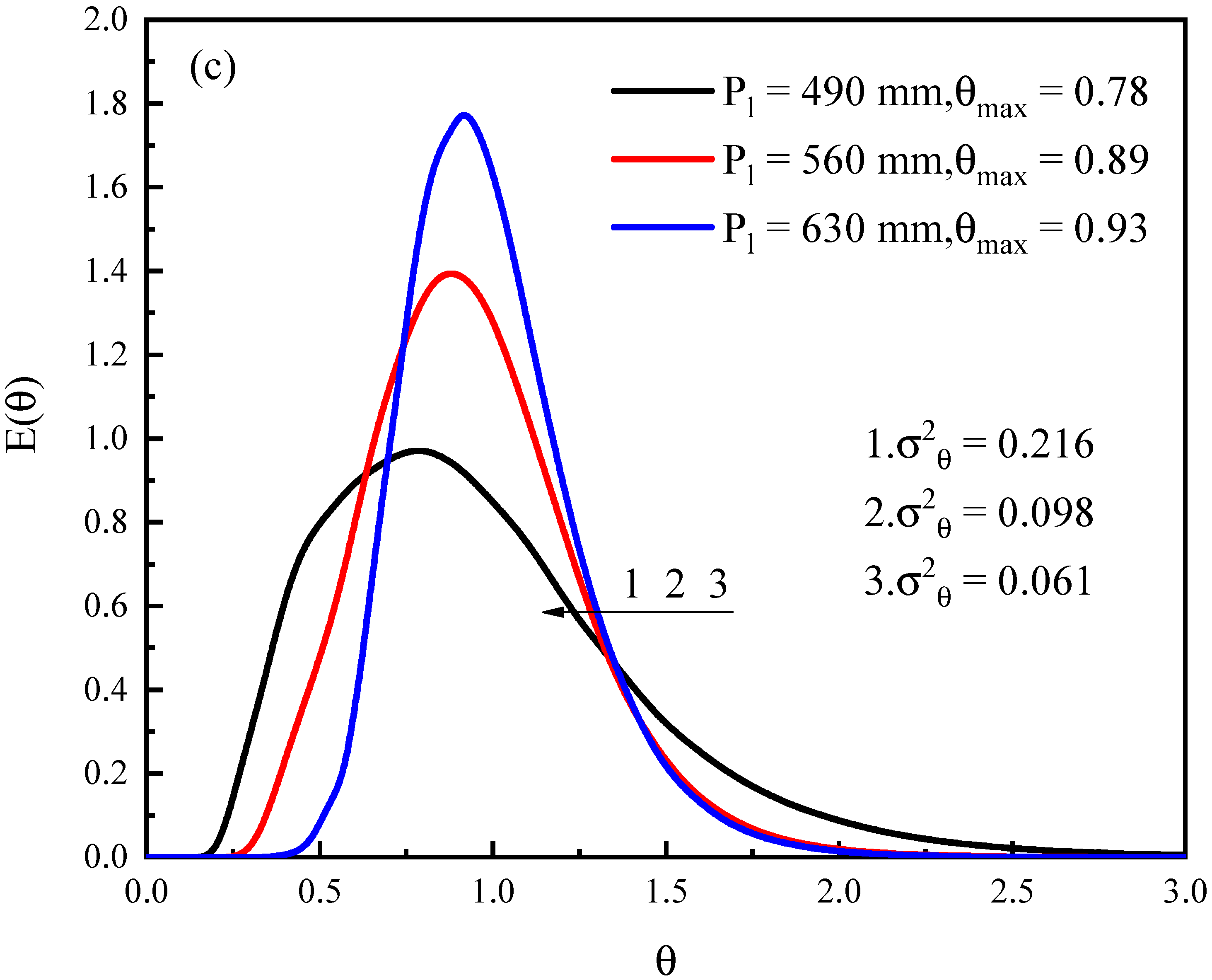
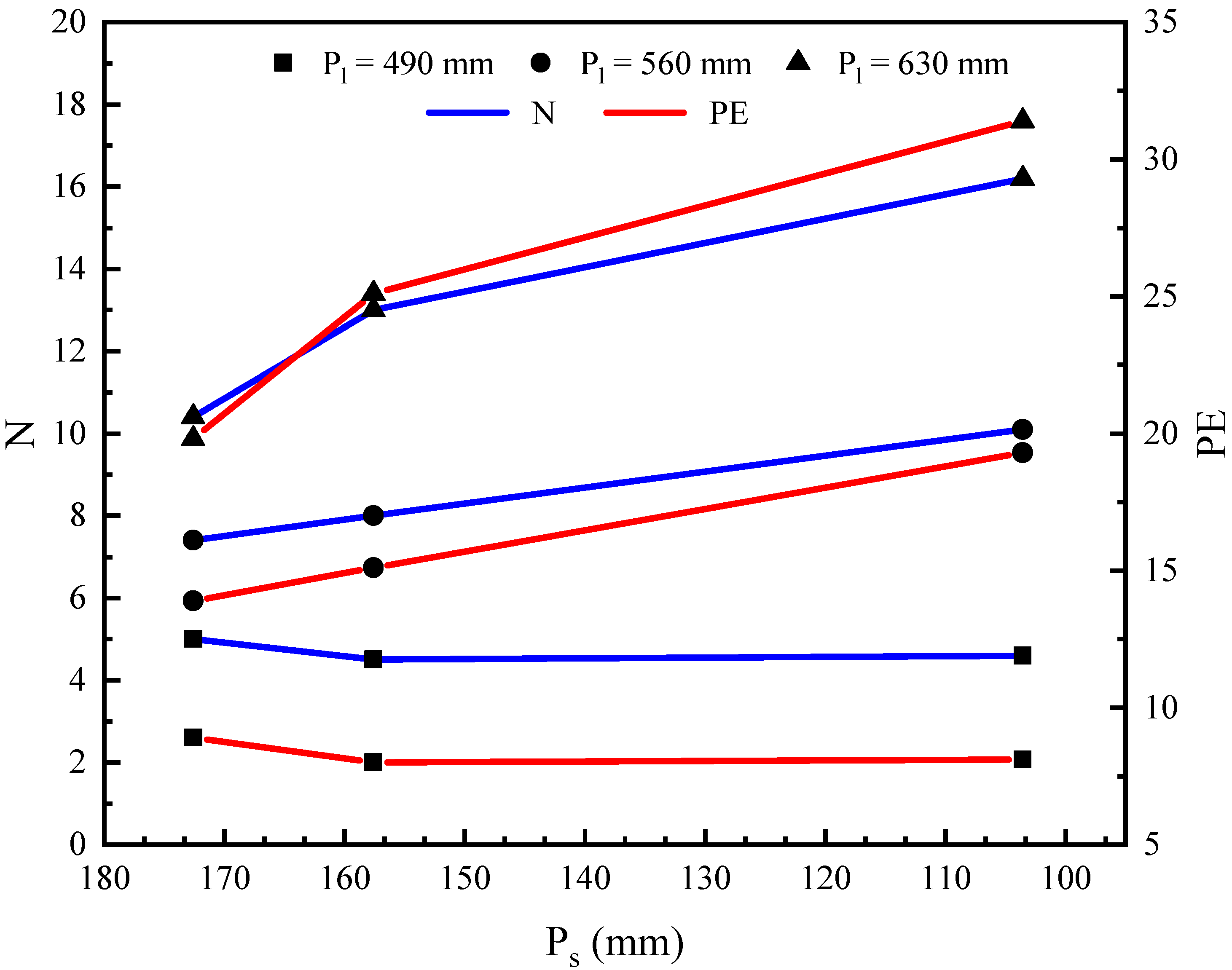
In order to quantitatively analyze the degree of backmixing in the reactor, the Pe number and model parameter N can be calculated based on the axial dispersion model and the tanks-in-series model to characterize the degree of backmixing, based on the dimensionless variance of the RTD curve. The calculated Pe numbers and model parameter N are shown in Table 3 and Figure 7. Table 3 shows that the overall numerical range of model parameter N is 4.5–16.2, which indicates that the flow state of the reactor is in the form of plug-flow according to its properties. Figure 7 shows that model parameter N always increases with the increase in plate height regardless of plate spacing, which also indicates that the backmixing in the reactor becomes smaller and smaller, and the flow state tends to be more in the form of plug-flow. Moreover, we find that the trend in Pe number is consistent with model parameter N. The larger Pe value indicates that the axial diffusion in the reactor is smaller and closer to the plug-flow, which also confirms our previous analysis of model parameter N. Therefore, within the scope of this experiment, we know that, in order to reduce the degree of backmixing, the height of the pole plate should be increased as much as possible. In addition, from the perspective of electrochemical descaling principles, increasing the pole plate area can effectively enhance the efficiency of electrochemical descaling [10,11].
Table 3.
Pe number and model parameter N.

Figure 7.
Plot of the effect of pole plate height on Pe number, model parameter N.
3.4. The Effect of Plate Spacing on the Reactor’s Hydraulic Characteristics
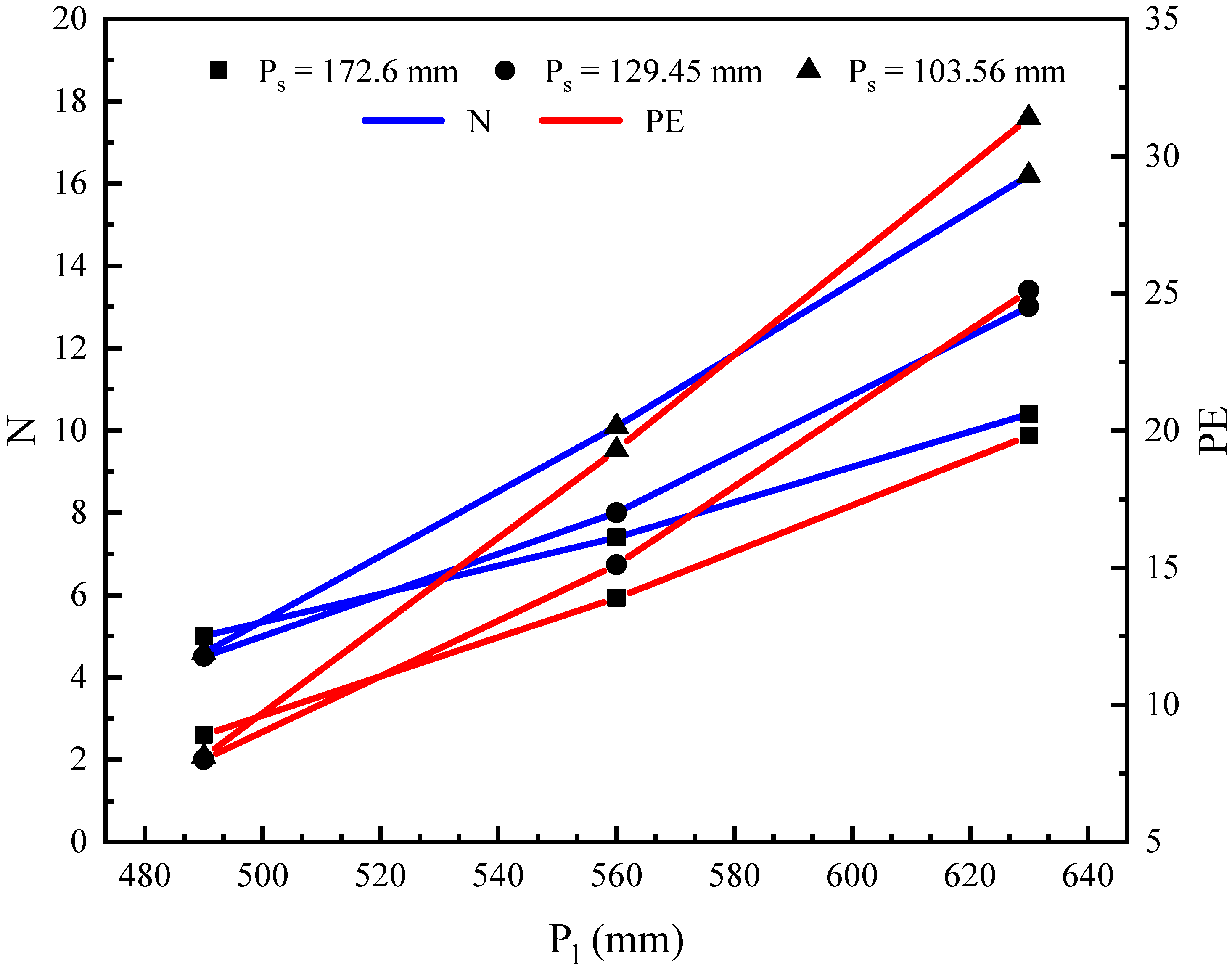
Figure 8 shows that the maximum peak time of the RTD curve increases to different degrees with the decrease in pole plate spacing at the same pole plate height. The changes in the maximum peak time were 0.776–0.786, 0.83–0.89, and 0.87–0.93 when the pole plate height was 490, 560, and 630 mm, respectively. Early peaking indicates that there is short-circuiting in the reactor. Part of the fluid flows out of the reactor without the reaction, resulting in reduced reaction efficiency. The increase in peak time indicates that reducing the pole plate spacing can reduce short-circuiting in the device within a certain range and improve the reaction conditions. The peak time was closer to 1 and the shape of the curve was closer to a normal distribution, which indicated that backmixing in the reactor was gradually decreasing. However, it is worth noting that the variance in RTD curves at different pole plate heights has different trends in relation to decreasing pole plate spacing. This can be seen in Figure 8a, where the variance of RTD curves increases from 0.198 to 0.217 and then decreases to 0.216. However, as can be seen in Figure 8b,c where the variance in RTD shows a monotonically decreasing trend with a decreasing pole plate spacing trend, this may be due to some coupling between the two. Since the pole plate spacing and pole plate height change to act on the fluid flow field, resulting in an interaction between the two and thus, showing different changes that ought to be investigated further in the future.
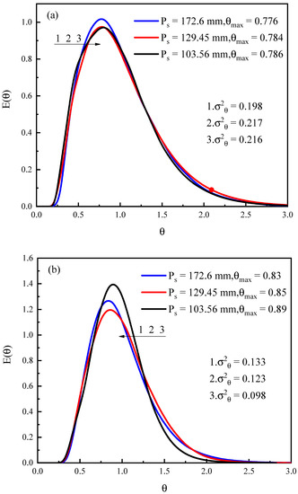
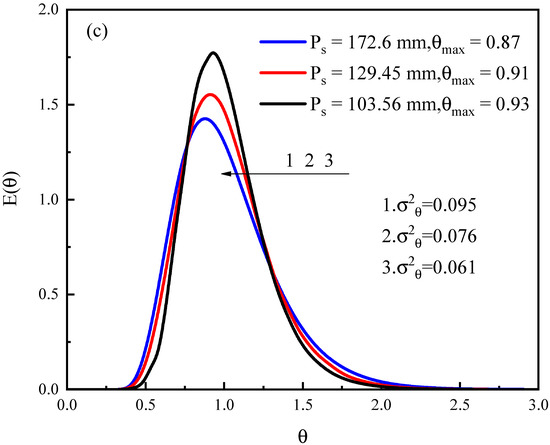
Figure 8.
Plot of the effect of pole plate spacing on the RTD curve ((a): The residence time distribution curves of the reactor when V is 2.6 m/s, Pl is 490 mm, and Ps is 172.6, 129.45 and 103.56 mm, respectively; (b): The residence time distribution curves of the reactor when V is 2.6 m/s, Pl is 560 mm, and Ps is 172.6, 129.45 and 103.56 mm, respectively; (c): The residence time distribution curves of the reactor when V is 2.6 m/s, Pl is 630 mm, and Ps is 172.6, 129.45 and 103.56 mm, respectively).
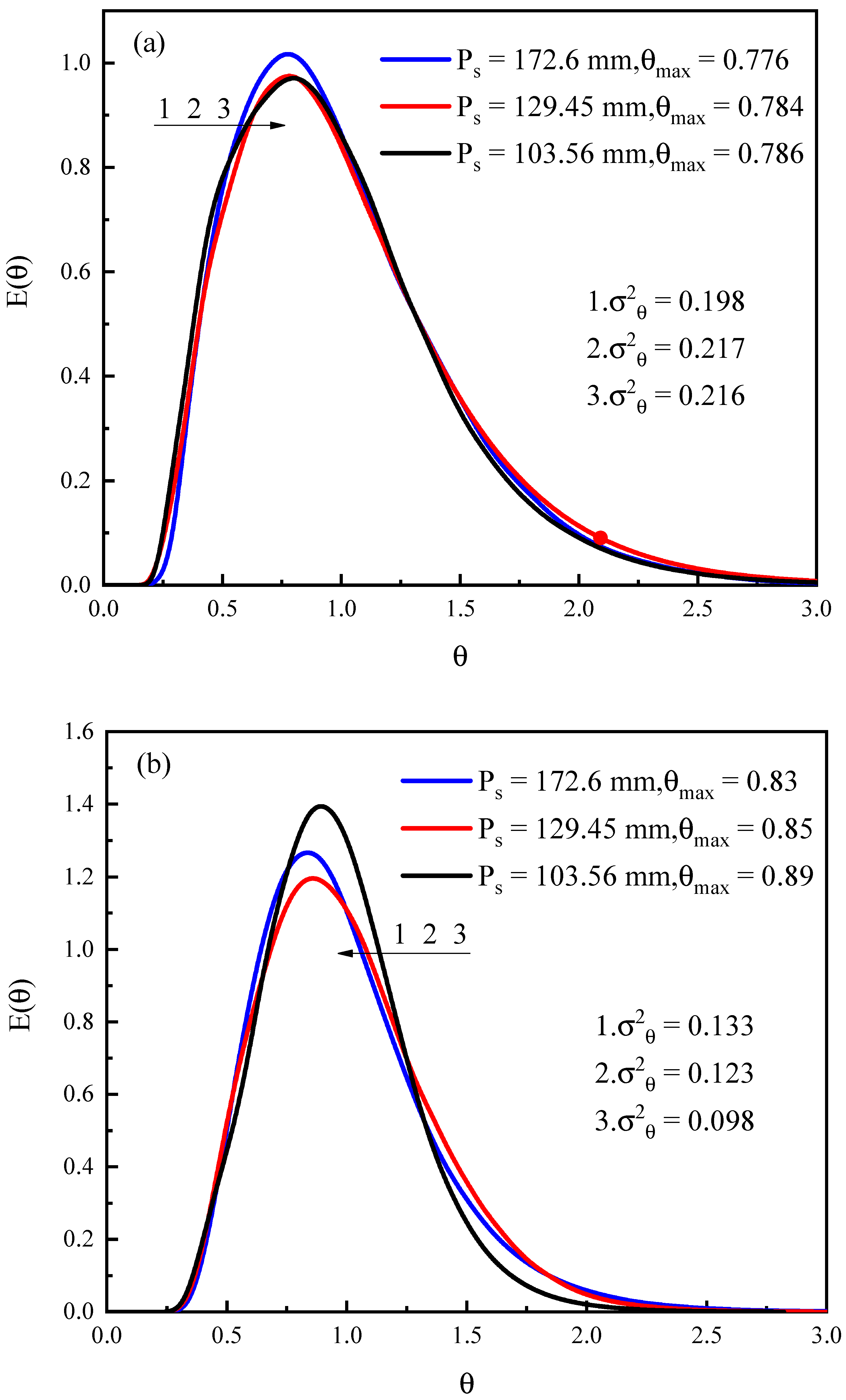
As shown in Figure 9, the Pe number represents the ratio of convection rate to diffusion rate. Through this, we can see that the backmixing in the reactor is small and the flow state is normal, i.e., it is between the horizontal flow and fully mixed flow. Model parameter N and the Pe number both increase with the decreasing plate spacing, which indicates that the decreasing plate spacing also suppresses the backmixing in the reactor and enhances the fluid pushing state.
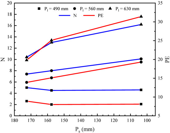
Figure 9.
Plot of the effect of pole plate spacing on Pe number and model parameter N.
3.5. Reactor Flow Field Characteristics and Analysis
In order to obtain more accurate simulation results in the spatial dimension, three-dimensional simulations of the electrochemical reactor were performed. However, it was often difficult to analyze the three-dimensional flow field. Therefore, we generally adopted the approach of selecting representative two-dimensional planes for later discussion.
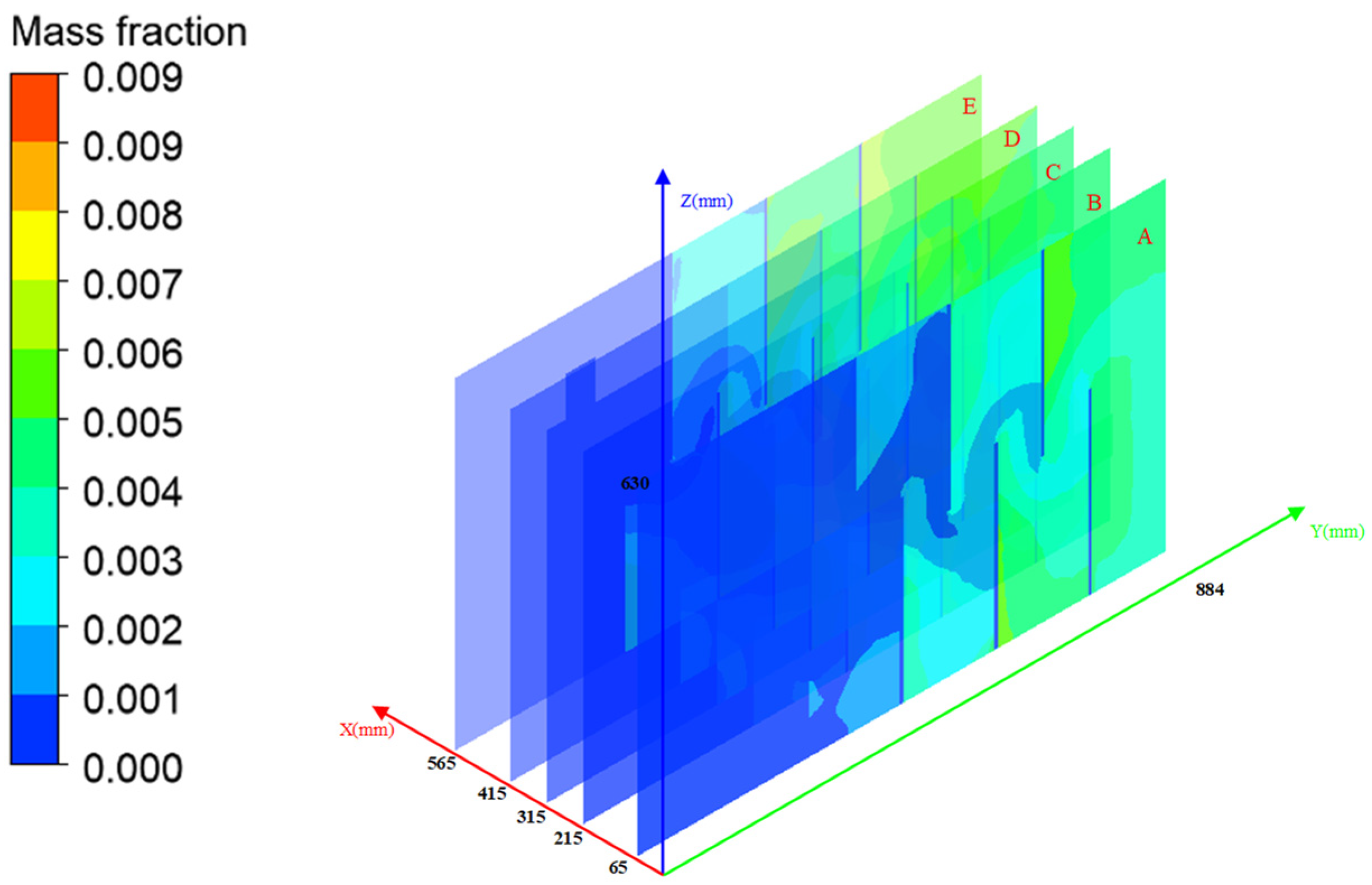
As shown in Figure 10, when the flow time is 80 s, we selected five sections in the YZ plane with X-axis values of 65, 215, 315, 415, and 565 mm, respectively. In order to observe more clearly the differences between the concentration nephogram of each cross-section, the concentration nephograms of each section in the frontal view of the YZ plane are plotted as shown in Figure 11. As can be seen from Figure 11, the concentration distribution pattern of the tracer and the size of the concentration gradient present at each location have a high similarity on sections A, B, and C. On the contrary, in sections D and E, the overall concentration size of section D does not differ much from sections A, B, and C, but its concentration distribution pattern is different, as shown in the red part of Figure 11D. The overall concentration of section E was clearly seen to be higher than the other four planes. In summary, section C was selected as the object of analysis in this following paper.
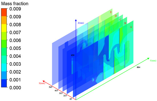
Figure 10.
Position of each section and contour plot of tracer concentration.
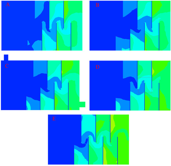
Figure 11.
Tracer concentration contour plot for the YZ-plane view in each section. ((A): Tracer concentration contour in YZ section when the X-axis value is 65 mm; (B): Tracer concentration contour in YZ section when the X-axis value is 215 mm; (C): Tracer concentration contour in YZ section when the X-axis value is 315 mm; (D): Tracer concentration contour in YZ section when the X-axis value is 415 mm; (E): Tracer concentration contour in YZ section when the X-axis value is 565 mm).
In order to obtain the universal characteristics of the reactor flow field, the calculation results were further analyzed by means of data visualization to lay the foundation for the subsequent reactor design and optimization. The velocity vector diagram obtained by post-processing is shown in Figure 12.
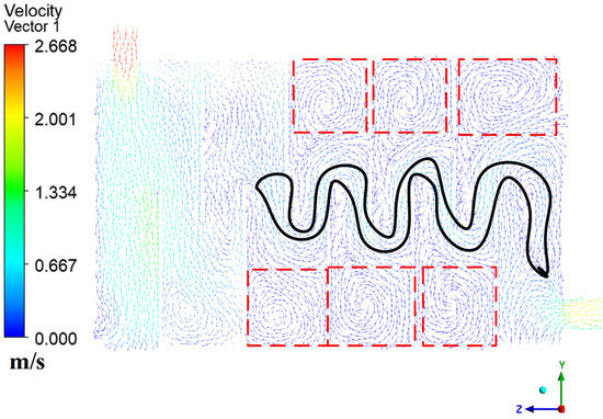
Figure 12.
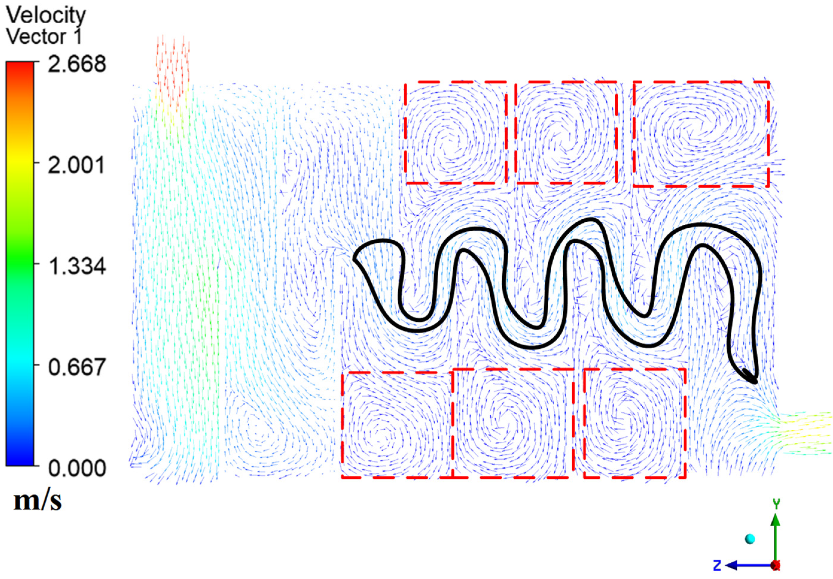
YZ plane velocity vector diagram of the reactor at x = 0.315 m (V = 2.6 m/s, Pl = 490 mm, Ps = 129.45 mm).
As can be seen from Figure 12, after the reaction fluid enters the reactor, part of the fluid flows out of the reactor with the shortest path and a faster speed due to the initial velocity and inertial force, as shown in the black area in the figure. For the reaction system, this indicates that the residence time of this part of the fluid in the reactor is short. Therefore, it does not ensure a sufficient reaction time and integrity of the reaction, which tends to affect the reaction efficiency. The other part of the fluid forms a vortex or stagnates in a certain area, as shown in red in the figure. These two areas are called the “ short-circuiting “ and the “dead zone”, which correspond to the two extremes of flow in the reaction, respectively. What we can find from the figure is that the short-circuit zone is generally closer to the head of the pole plate, while the dead zone is generally located between the pole plates or at the corners of the reactor. Therefore, RTD tracing experiments were conducted to verify the accuracy and universality of this phenomenon.
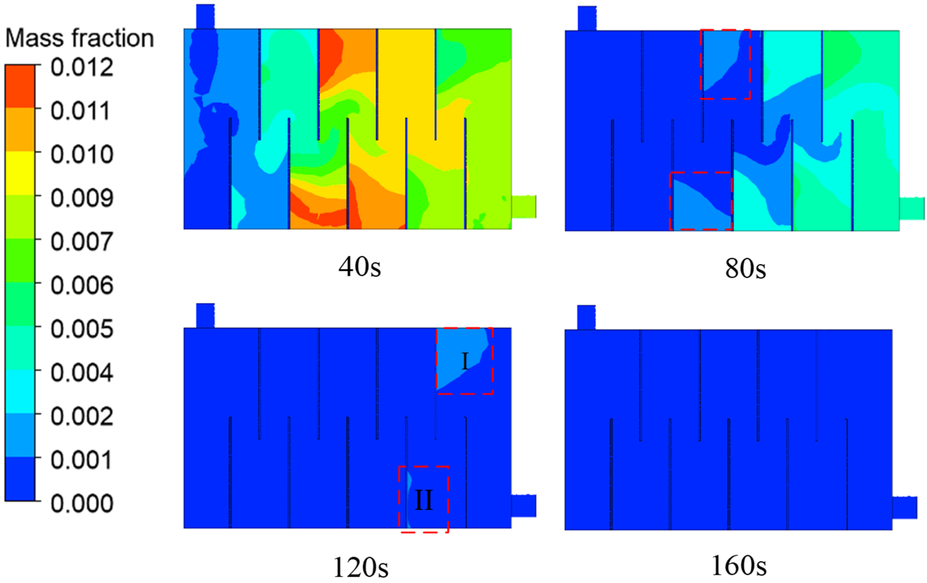
As can be seen from Figure 13, when the reaction reaches 40 s, there is a spread of tracer concentration in all of the places inside the reactor, which indicates that the tracer has been fully mixed with the material by the fluid flow, as well as its own diffusion. Due to a different rate of entrainment of the main fluid in different regions of the chamber, various tracer micro-elements in different zones have different residence times. When the reaction reaches 80 s, we can see a concentration gradient in the red box part of the figure, which indicates that most of the tracer at this location has left the forward flow. However, there is still a part of the tracer that is stagnant at this location and there is a more obvious concentration gradient, which also indicates that this location is the reactor dead zone. When the reaction proceeds to 120 s, we can see that the tracer in all of the areas of the reactor, including the outlet, has exited the system. However, there are still tracers in the two corners that remain in the system and their positions change as compared to 80 s. Among them, the retention volume in area I is higher, which can be interpreted as the hydraulic dead zone. In area II, the retention volume is lower, which may be caused by the time dependent nature of flow, etc. When the reaction proceeds to 160 s, we can see that the tracer concentration in the system is 0, and we can assume that the tracer has exited the system. From the above analysis, it can be seen that, due to the reactor’s structure, there is a small dead zone in the reactor. This is most likely found in the narrow area between the pole plates, which is also consistent with the vortex generation phenomenon in Figure 12.
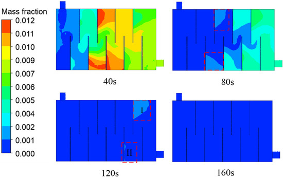
Figure 13.
Contour plot of the YZ plane tracer concentration at x = 315 mm with time for the reactor (V = 2.6 m/s, Pl = 490 mm, Ps = 129.45 mm).
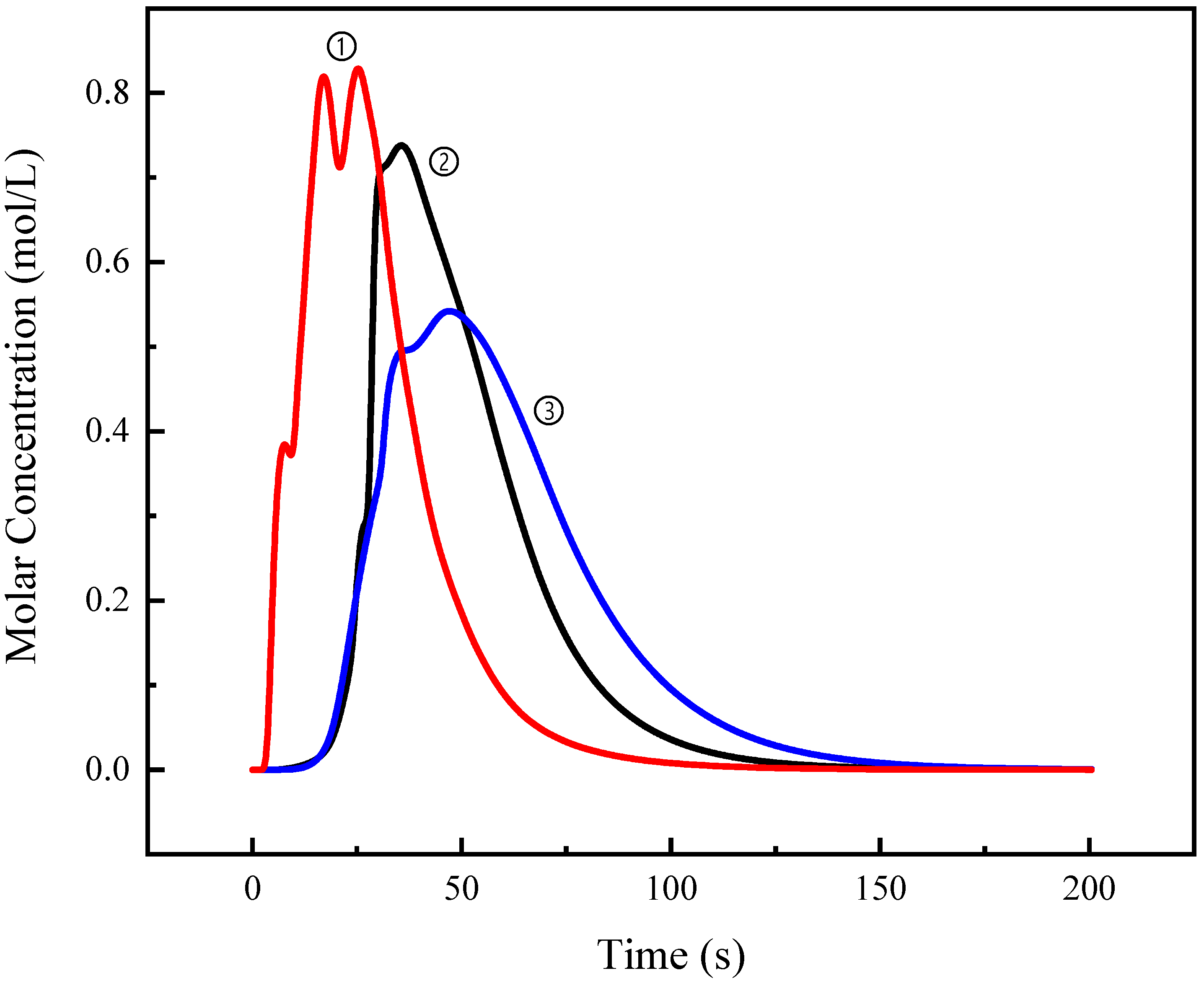
In order to further study the reactor hydraulic characteristics, three observation points located at the corners of the reactor and the head of the pole plate were selected according to the above analysis. In addition, their concentration variation curves with time were monitored and analyzed. The locations of the measurement points are shown in Figure 14, and the monitoring data were plotted to obtain Figure 15.
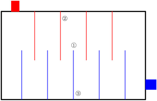
Figure 14.
Schematic diagram of the position of each measurement point in the reactor.
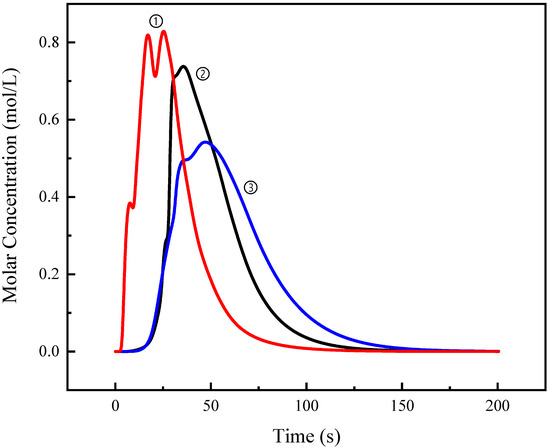
Figure 15.
Concentration curve of each measurement point with time.
As seen in Figure 15, there are certain similarities between the shape of the concentration curve and the residence time distribution at each point. The measurement point 1 is located at the head of the pole plate. In addition, its concentration curve shows a double peak characteristic. It indicates the presence of two parallel fluids or the existence of a short-circuit and a trench flow simultaneously, in agreement with the previous analyses. Moreover, one can notice that the peaks of the two peaks are not exactly the same. This is due to the different concentrations of tracer within the two fluids, resulting in slightly different concentration magnitudes. Whereas, Points 2 and 3 are located at the corners of the reactor, and show the late arrival of the peaks and slower decay in the concentration. This is evidence that some of the fluid has been recirculating in the reactor for a long time. Therefore, a dead zone formation occurred.
3.6. Energy Consumption Analysis
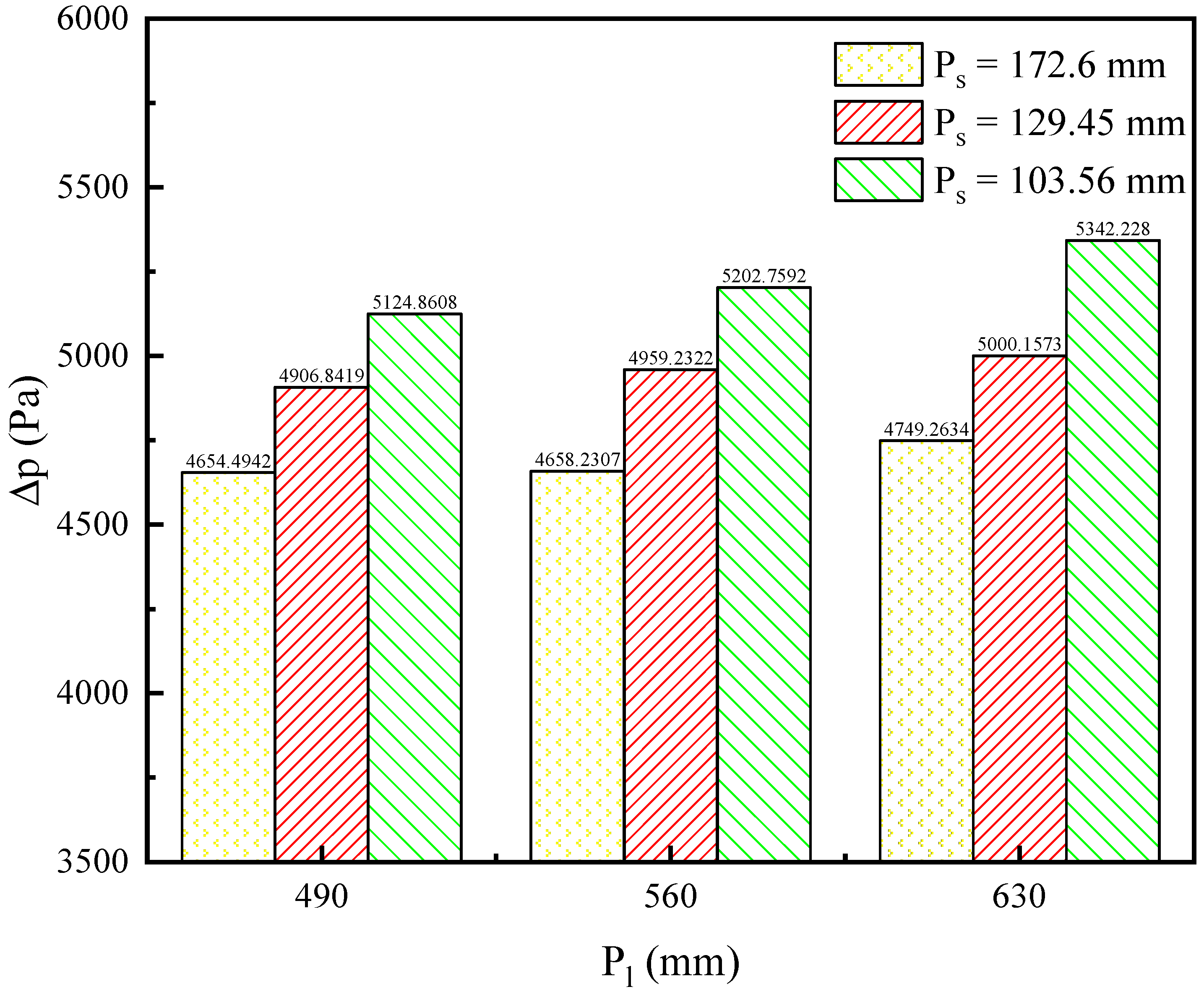
While analyzing the effect of the reactor’s structure on its hydraulic characteristics, the energy consumption during the operation must also be considered, as lower energy consumption can effectively reduce the treatment cost. Therefore, the inlet and outlet pressure drops during the operation of the reactor under different structures were monitored, and the results are shown in Figure 16.
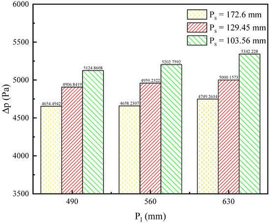
Figure 16.
Schematic diagram of pressure drop changes under different working conditions.
Figure 16 shows that, with the increase in the height of the pole plate, the pressure drop shows a slowly growing trend. The maximum pressure increase values are 94, 93, and 217 Pa, for an increase in pole height from 490 to 630 mm, when the pole plate spacing is kept constant at 172.6, 129.45, and 103.56 mm, respectively. However, as the pole plate spacing decreases, we can clearly see that the growth of pressure drop becomes more significant. The maximum pressure increase values are 470, 544, and 592 Pa, for a decrease in pole plate spacing from 172.6 to 103.56 mm, when the pole plate height is kept constant at 490, 560, and 630 mm, respectively. This indicates that either the increasing plate height or decreasing plate spacing can increase the energy consumption of the reaction, which has been reported in many studies [40,41,42]. However, another conclusion that can be drawn from the analysis of specific values is that the increasing plate height has a much lower impact on energy consumption than the decreasing plate spacing. Moreover, this provides a strong theoretical support for the subsequent optimization of the reactor.
4. Conclusions
In this paper, we investigated a three-dimensional simulation of fluid flow in electrochemical descaling reactors with different structures using CFD, as well as reactor hydraulic characteristics, fluid flow field, and residence time distribution. The following conclusions are obtained:
- The verification of grid independence and the verification of the flow field reaching a steady-state were carried out for the numerical simulation to reduce the rounding error and to ensure that the experimental conditions were established, which ensured the accuracy of the numerical simulation results.
- The qualitative analysis of the reactor flow characteristics and the degree of backmixing by analyzing the RTD curves showed that increasing the plate height and decreasing the plate spacing could reduce the reactor backmixing and make it more similar to the plug-flow. The trend in increasing the maximum peak time and making it more similar to the average residence time was observed, which could effectively improve the bad flow.
- The simulation experiment can predict the fluid flow field distribution characteristics and tracer concentration in a reactor. By observing the flow field of the reactor, it was found that there were dead zones and short-circuiting in the reactor (Pl = 129.45 mm, Ps = 490 mm). In addition, the distribution characteristics of dead zones and short-circuiting were obtained by analyzing the contour plot of tracer concentration and monitoring the measurement points.
- In the electrochemical descaling reactor studied in this paper, both increasing the plate height and decreasing the plate spacing can effectively reduce the undesirable flow patterns during the reaction process, as well as enhance the reaction efficiency. However, both changes increase the reactor pressure drop and thus, increase the energy loss. Moreover, the effect of increasing the plate height on energy consumption was much smaller than decreasing the plate spacing. Therefore, in this case, we need to make a more balanced choice regarding the efficiency and energy consumption when designing and optimizing the reactors. During the optimization of a reactor, one should consider increasing the height of the pole plate as much as possible to improve the reactor’s performance and, at the same time, reduce the expenditure.
In this paper, the performance optimization conditions of the reactor were investigated from the perspective of reactor hydraulic characteristics using the CFD method, and preliminary conclusions were obtained. However, it is still in the laboratory stage, and the specific application effect is still unclear. In order to better apply the research results to practice, further medium-sized experiments are needed to guide the next theoretical research with practical effects. Moreover, simulation can be carried out from additional angles to improve the reaction efficiency of the reactor, such as simulating the chemical reaction process of descaling, and the influence of temperature, calcium ion concentration, and other factors on the reaction.
Author Contributions
Conceptualization, B.H. and X.Z.; writing—original draft preparation, B.H.; Writing—review & editing, B.H., Z.W. (Zhaofeng Wang) and Y.J.; Visualization, B.H.; Funding acquisition, X.Z.; Resources, X.Z.; Supervision, X.Z.; Formal analysis, Z.W. (Zixian Wang). All authors have read and agreed to the published version of the manuscript.
Funding
This work was supported by the Natural Science Foundation of China (grant no. 51804270), the Natural Science Foundation of Hunan Province (grant no. 2020JJ5547), and the Research Fund of Hunan Provincial Department of Education (grant no. 19C1745).
Institutional Review Board Statement
Not applicable.
Informed Consent Statement
Not applicable.
Data Availability Statement
The data presented in this study are available in hydraulic characteristics, residence time distribution, and flow field of electrochemical descaling reactor using CFD.
Conflicts of Interest
The authors declare no conflict of interest.
References
- National Bureau of Statistics of China, China Statistical Yearbook. 2021. Available online: https://data.stats.gov.cn/easyquery.htm?cn=C01 (accessed on 31 August 2021).
- Bao, Q. Circulating cooling water treatment over the last thirty years in China. Ind. Water Treat. 2010, 30, 6–14. [Google Scholar]
- Hasson, D.; Sidorenko, G.; Semiat, R. Calcium Carbonate Hardness Removal by a Novel Electrochemical Seeds System. Desalination 2010, 263, 285–289. [Google Scholar] [CrossRef]
- Zhi, S.; Zhang, K. Hardness Removal by a Novel Electrochemical Method. Desalination 2016, 381, 8–14. [Google Scholar] [CrossRef]
- Zhang, C.; Tang, J.; Zhao, G.; Tang, Y.; Li, J.; Li, F.; Zhuang, H.; Chen, J.; Lin, H.; Zhang, Y. Investigation on an Electrochemical Pilot Equipment for Water Softening with an Automatic Descaling System: Parameter Optimization and Energy Consumption Analysis. J. Clean. Prod. 2020, 276, 123178. [Google Scholar] [CrossRef]
- Gabrielli, C.; Maurin, G.; Francy-Chausson, H.; Thery, P.; Tran, T.T.M.; Tlili, M. Electrochemical Water Softening: Principle and Application. Desalination 2006, 201, 150–163. [Google Scholar] [CrossRef]
- Hasson, D.; Lumelsky, V.; Greenberg, G.; Pinhas, Y.; Semiat, R. Development of the Electrochemical Scale Removal Technique for Desalination Applications. Desalination 2008, 230, 329–342. [Google Scholar] [CrossRef]
- Janssen, L. The Role of Electrochemistry and Electrochemical Technology in Environmental Protection. Chem. Eng. J. 2002, 85, 137–146. [Google Scholar] [CrossRef]
- Guo, Y.; Xu, Z.; Guo, S.; Chen, S.; Xu, H.; Xu, X.; Gao, X.; Yan, W. Selection of Anode Materials and Optimization of Operating Parameters for Electrochemical Water Descaling. Sep. Purif. Technol. 2021, 261, 118304. [Google Scholar] [CrossRef]
- Luan, J.; Wang, L.; Sun, W.; Li, X.; Zhu, T.; Zhou, Y.; Deng, H.; Chen, S.; He, S.; Liu, G. Multi-Meshes Coupled Cathodes Enhanced Performance of Electrochemical Water Softening System. Sep. Purif. Technol. 2019, 217, 128–136. [Google Scholar] [CrossRef]
- Hasson, D.; Sidorenko, G.; Semiat, R. Low Electrode Area Electrochemical Scale Removal System. Desalination Water Treat. 2011, 31, 35–41. [Google Scholar] [CrossRef]
- Weinert, F.M.; Braun, D. Observation of Slip Flow in Thermophoresis. Phys. Rev. Lett. 2008, 101, 168301. [Google Scholar] [CrossRef] [Green Version]
- Mattia, D.; Leese, H.; Calabrò, F. Electro-Osmotic Flow Enhancement in Carbon Nanotube Membranes. Philos. Trans. R. Soc. A Math. Phys. Eng. Sci. 2016, 374, 20150268. [Google Scholar] [CrossRef] [PubMed] [Green Version]
- Aminpour, M.; Torres, S.A.G.; Scheuermann, A.; Li, L. Slip-Flow Regimes in Nanofluidics: A Universal Superexponential Model. Phys. Rev. Appl. 2021, 15, 054051. [Google Scholar] [CrossRef]
- Ríos, D.A.; Toro Vélez, A.F.; Peña, M.R.; Parra, C.A.M. Changes of Flow Patterns in a Horizontal Subsurface Flow Constructed Wetland Treating Domestic Wastewater in Tropical Regions. Ecol. Eng. 2009, 35, 274–280. [Google Scholar] [CrossRef]
- Danckwerts, P.V. Continuous Flow Systems: Distribution of Residence Times. Chem. Eng. Sci. 1953, 2, 1–13. [Google Scholar] [CrossRef]
- Levenspiel, O. Chemical Reaction Engineering; Wiley: New York, NY, USA, 1962. [Google Scholar]
- Makokha, A.B.; Moys, M.H.; Bwalya, M.M. Modeling the RTD of an Industrial Overflow Ball Mill as a Function of Load Volume and Slurry Concentration. Miner. Eng. 2011, 24, 335–340. [Google Scholar] [CrossRef]
- Ding, J.; Wang, X.; Zhou, X.-F.; Ren, N.-Q.; Guo, W.-Q. CFD Optimization of Continuous Stirred-Tank (CSTR) Reactor for Biohydrogen Production. Bioresour. Technol. 2010, 101, 7005–7013. [Google Scholar] [CrossRef]
- Das, S.; Sarkar, S.; Chaudhari, S. Modification of UASB Reactor by Using CFD Simulations for Enhanced Treatment of Municipal Sewage. Water Sci. Technol. 2017, 77, 766–776. [Google Scholar] [CrossRef]
- Hurtado, J.P.; Villegas, B.; Pérez, S.; Acuña, E. Optimization Study of Guide Vanes for the Intake Fan-Duct Connection Using CFD. Processes 2021, 9, 1555. [Google Scholar] [CrossRef]
- Xie, Q.; Zheng, M. CFD Simulation and Performance Investigation on a Novel Bionic Spider-Web-Type Flow Field for PEM Fuel Cells. Processes 2021, 9, 1526. [Google Scholar] [CrossRef]
- Yang, R.; Sun, X.; Liu, Z.; Zhang, Y.; Fu, J. A Numerical Analysis of the Effects of Equivalence Ratio Measurement Accuracy on the Engine Efficiency and Emissions at Varied Compression Ratios. Processes 2021, 9, 1413. [Google Scholar] [CrossRef]
- Chen, G. Chemical Reaction Engineering; Chemical Industry Press: Beijing, China, 1989. [Google Scholar]
- Zhang, C.; Li, S.; Wang, Z.; Shen, Y.; Wei, F. Model and Experimental Study of Relationship between Solid Fraction and Back-Mixing in a Fluidized Bed. Powder Technol. 2020, 363, 146–151. [Google Scholar] [CrossRef]
- Shi, X.; Sun, R.; Lan, X.; Liu, F.; Zhang, Y.; Gao, J. CPFD Simulation of Solids Residence Time and Back-Mixing in CFB Risers. Powder Technol. 2015, 271, 16–25. [Google Scholar] [CrossRef]
- Shah, Y.T.; Stiegel, G.J.; Sharma, M.M. Backmixing in Gas-Liquid Reactors. AIChE J. 1978, 24, 369–400. [Google Scholar] [CrossRef]
- Tobita, H. Continuous Free-Radical Polymerization with Long-Chain Branching and Scission in a Tanks-in-Series Model. Macromol. Theory Simul. 2014, 23, 182–197. [Google Scholar] [CrossRef]
- Jafarikojour, M.; Sohrabi, M.; Royaee, S.J.; Rezaei, M. A New Model for Residence Time Distribution of Impinging Streams Reactors Using Descending-Sized Stirred Tanks in Series. Chem. Eng. Res. Des. 2016, 109, 86–96. [Google Scholar] [CrossRef]
- Chrismianto, D.; Kim, D.-J. Parametric Bulbous Bow Design Using the Cubic Bezier Curve and Curve-Plane Intersection Method for the Minimization of Ship Resistance in CFD. J. Mar. Sci. Technol. 2014, 19, 479–492. [Google Scholar] [CrossRef]
- Ruggiero, A.; D’Amato, R.; Affatato, S. Comparison of Meshing Strategies in THR Finite Element Modelling. Materials 2019, 12, 2332. [Google Scholar] [CrossRef] [Green Version]
- Farhadian, N.; Behin, J.; Parvareh, A. Residence Time Distribution in an Internal Loop Airlift Reactor: CFD Simulation versus Digital Image Processing Measurement. Comput. Fluids 2018, 167, 221–228. [Google Scholar] [CrossRef]
- González-Juárez, D.; Solano, J.P.; Herrero-Martín, R.; Harvey, A.P. Residence Time Distribution in Multiorifice Baffled Tubes: A Numerical Study. Chem. Eng. Res. Des. 2017, 118, 259–269. [Google Scholar] [CrossRef]
- Jones, W.P.; Launder, B. The Calculation of Low-Reynolds-Number Phenomena With a Two-Equation Model of Turbulence. Int. J. Heat Mass Transf. 1973, 16, 1119–1130. [Google Scholar] [CrossRef]
- Jones, W.P.; Launder, B. The Prediction of Laminarization with a Two-Equation Model of Turbulence. Int. J. Heat Mass Transf. 1972, 15, 301–314. [Google Scholar] [CrossRef]
- Zhang, Y.; Wang, Z.; Jin, Y.; Li, Z.; Yi, W. CFD Simulation and Experiment of Residence Time Distribution in Short-Contact Cyclone Reactors. Adv. Powder Technol. 2015, 26, 1134–1142. [Google Scholar] [CrossRef]
- Guenther, C.; Syamlal, M.; Shadle, L.; Ludlow, C. A Numerical Investigation of an Industrial Scale Gas-Solids CFB. Circ. Fluid. Bed Technol. 2002, 25, 483–488. [Google Scholar]
- Hua, L.; Wang, J.; Li, J. CFD Simulation of Solids Residence Time Distribution in a CFB Riser. Chem. Eng. Sci. 2014, 117, 264–282. [Google Scholar] [CrossRef]
- Zhou, Q.; Wang, J.; Li, J. Three-Dimensional Simulation of Dense Suspension Upflow Regime in High-Density CFB Risers with EMMS-Based Two-Fluid Model. Chem. Eng. Sci. 2014, 107, 206–217. [Google Scholar] [CrossRef]
- Jian, W.; Huizhu, Y.; Wang, S.; Xu, S.; Yulan, X.; Tuo, H. Numerical Investigation on Baffle Configuration Improvement of the Heat Exchanger with Helical Baffles. Energy Convers. Manag. 2015, 89, 438–448. [Google Scholar] [CrossRef]
- Kumar, R.; Sethi, M.; Chauhan, R.; Kumar, A. Experimental Study of Enhancement of Heat Transfer and Pressure Drop in a Solar Air Channel with Discretized Broken V-Pattern Baffle. Renew. Energy 2017, 101, 856–872. [Google Scholar] [CrossRef]
- Promvonge, P. Heat Transfer and Pressure Drop in a Channel with Multiple 60° V-Baffles. Int. Commun. Heat Mass Transf. 2010, 37, 835–840. [Google Scholar] [CrossRef]


Publisher’s Note: MDPI stays neutral with regard to jurisdictional claims in published maps and institutional affiliations. |
© 2021 by the authors. Licensee MDPI, Basel, Switzerland. This article is an open access article distributed under the terms and conditions of the Creative Commons Attribution (CC BY) license (https://creativecommons.org/licenses/by/4.0/).