Integral Layout Optimization of Subsea Production Control System Considering Three-Dimensional Space Constraint

Abstract

The subsea production control system, characterized by a complex and diverse structure and high cost, is one of the essential parts of a subsea production system. The rational layout of the subsea production control system is essential to reduce development costs and ensure safe production in offshore fields. Most previous studies on layout design in offshore fields have focused on the oil- and gas-gathering system. However, the layout of the subsea production control system has not thoroughly been researched to date and the seabed terrain and integral optimization have rarely been discussed. This paper focuses on the multi-layer star structure and multi-layer star-tree structure, two common layout structures of subsea production control systems, and establishes the corresponding model with obstacle and seabed terrain conditions. Obtaining the lowest possible total cost was the aim of the model. A hybrid algorithm combining the adaptive mutation particle swarm algorithm and the A-star algorithm was applied to integrally optimize the subsea distribution unit and umbilical touch down point positions, the pipe connection topology and pipe routes. The practicality of this approach is demonstrated by designing a layout with one FPSO and 22 subsea control modules. The results indicate that the multi-layer star-tree layout structure has a lower total cost compared to that of the multi-layer star layout structure. In addition, the results were compared with a case that ignores the seabed terrain, indicating differences in the total construction cost. This method provides engineers with quantitative references and reliable cost estimates to make decisions regarding the layout of the subsea production control system.

1. Introduction

Oil and gas resources are among the key supporting pillars of economic development. Oil and gas production plays an important role in national development and social progress. Due to the significance of oil and gas resources and the increasing scarcity of oil resources on land, oil and gas producers are increasingly exploiting offshore oil and gas fields. By 1995, offshore oil production accounted for nearly 30% of the world’s oil production [1]. With the increasing depth of the exploration of offshore oil and gas resources, using a subsea production system and FPSO is gradually becoming the mainstream development model in offshore fields. This development model has attracted widespread attention from various countries for its advantages such as its higher recovery rate, faster development speed and considerable economic benefits. At present, deep-water oil and gas fields in the Gulf of Mexico and Brazil have adopted this development model [2,3,4,5,6]. However, the expensive development costs of offshore oil and gas fields and persistently low oil prices have had a huge influence on offshore oil development. Reducing the construction cost of offshore fields is an effective strategy to cope with low oil prices. The layout optimization of the subsea production system is an effective solution to reduce field construction costs [7].

The subsea production system is composed of the oil- and gas-gathering system and the subsea production control system [8]. The oil- and gas-gathering system collects the oil and gas produced by the X-trees through the manifold, and then transports the oil and gasto the FPSO through the flowline. The subsea production control system remotely controls the X-tree and manifold to ensure the successful transport of the oil and gas from the seabed to the FPSO. The subsea production control system is mainly composed of an umbilical, flying line, subsea distribution unit (SDU) and a subsea control module (SCM), where the umbilical and fly line constitute the functional pipeline, and the SDU and SCM constitute the subsea control facility. The control process is to transmit the control signals (electrical and hydraulic signals) from the FPSO to the SDU through the umbilical and then to the SCM through the flying line. The SCM controls valves on X-trees and manifolds, collects the real-time production data of oil and gas reservoirs, and monitors the working conditions of the subsea production system to ensure safe production in offshore oilfields [9,10]. Therefore, the subsea production control system is an important part of the subsea production system. Furthermore, its construction cost is quite expensive. However, the current research focuses on the layout optimization of the oil- and gas-gathering system to reduce construction costs, as few studies have researched the layout of the subsea production control system. In order to further reduce the construction cost of offshore fields and to ensure the safe operation of subsea production systems, it is necessary to research the layout optimization of the subsea production control system.

The layout of the subsea production control system depends on the interconnection between control facilities which determines the layout structure of the functional pipelines and thus affects the cost. Cui et al. [11] proposed a method to optimize four pipe topological structures with a minimum annual total cost. Duan et al. [12] used the genetic algorithm and ant colony algorithm to optimize the topology of four gas field gathering pipeline layout structures. Zhang et al. [13] established a unified mixed integer linear programming model considering the terrain and obstacle conditions to optimize three pipe layout structures. The above studies show that the cost of various pipe layout structures differ greatly. Zhang et al. [14] optimized the layout of the offshore field gathering system considering the gathering radius, flow rate, terrain obstacles and production process. The similarity among the above studies is that the facilities’ locations are fixed and only the connections between facilities were optimized. Wang et al. [15] and Wu et al. [16] optimized the layout of industrial plants with both the locations of facilities and pipe connection topology, demonstrating that the location of facilities might affect the pipe connection topology and thus affect the cost. Based on the above description, it could be deduced that for the layout of subsea production control system, the pipe layout structure and integral optimization of the facility location and pipe connection topology could affect the total cost. Thus, for different pipe layout structures, the integral optimization of the facility location and pipe connection topology might further reduce the cost.

For the layout optimization of the offshore oil- and gas-gathering system, the integral optimization of the manifold location and pipeline connection topology has been studied in recent years. Rodrigues et al. [17] established a 0–1 linear programming model to obtain the position of FPSO and the manifold and the connection relationship between them. Silva et al. [18] proposed a mathematical model of mixed-integer linear programming to integrate the subsea production system, which determines the number, capacity, and location of platforms and manifolds, as well as the connection relationships of these facilities to minimize construction costs. Wang et al. [19] developed a model for the division of wells to determine the location of the manifolds and their connection relationships with the wells. Then, a new model was proposed to optimize the location and number of manifolds and the connection relationship with FPSO and manifolds [20]. Then, the layout was synergistically optimized by considering the location of the manifolds, wellhead groupings, and the connection relationships between the manifolds, while developing an iterative algorithm that integrates unsupervised learning methods and clustering algorithms to optimize the problem [21]. Liu et al. [22] established an MINLP model to optimize the position of the manifold and converted the MINLP model into a binary linear programming model in order to efficiently solve the model. However, the above situations did not consider the seabed terrain and obstacles, so the interconnections between the facilities is perceived as straight lines which will affect the layout result. Therefore, the routes of the functional pipeline should be designed in the layout of the subsea production control system.

Table 1. Comparisons between recent studies investigating the layout problem.

References	Application	Space	Advantage	Disadvantage
Cui et al. [11]	Pipe network layout	2D	Layout for four types of pipe network considering pipe reliability	3D terrain not considered; no integral optimization
Duan et al. [12]	Pipe network layout	3D	Considered 3D terrain and layout for four types of pipe network	No integral optimization; no optimal solution obtained
Zhang et al. [13]	Layout of oil-gathering pipe network	3D	Proposed unified MILP model and considered 3D terrain	No optimal solution was obtained
Zhang et al. [14]	Layout of subsea oil-gathering system	3D	Proposed MILP model considering pressure loss in the pipe	No optimization of the pipeline route; no optimal solution obtained
Wang et al. [15]	Layout of industrial plants	2D	Proposed a hybrid algorithm for coupling optimization	3D terrain not considered
Silva et al. [18]	Layout of subsea oil-gathering system	2D	Integral optimization of FPSO and subsea oil-gathering system	The pipe route was not optimized, which made the layout inaccurate
Wang et al. [21]	Layout of subsea oil-gathering system	2D	Proposed an algorithm for integral optimization	3D terrain not considered and inaccurate layout
Liu et al. [22]	Layout of subsea oil-gathering system	2D	Established MINLP optimization model and simplified model	Due to simplified model, optimal layout could not be obtained

illustrates the recent studies researching the layout problem.

In recent decades, the design of the subsea pipe route has attracted much attention. Lucena et al. [23] used the genetic algorithm to design subsea pipe routes, considering the seabed terrain, obstacles, and stability with the minimum pipeline length. Baioco et al. [24] set the minimum pipe length and the maximum oil production as a multi-objective function and optimized the pipe route, considering the seabed terrain and the pipeline stability. Kang et al. [25] proposed a method for the automatic obstacle avoidance of the pipeline route and applied the Laplacian smoothing algorithm to smooth the routes. Cheng et al. [26] established a nonlinear optimization model to design the pipe route with a minimal length that considers obstacles, seabed terrain and pipeline curvature, and the PSO-based augmented Lagrangian method was adapted to resolve the presented model. The construction expense of subsea pipelines accounts for a considerable proportion of the total development investment in offshore fields [27]. Therefore, it is extremely necessary to optimize the pipeline routes during the layout of the subsea production control system.

From the above review, two factors were found to affect the layout cost. The first factor is that the location of the facilities, pipe connection topology and pipe routes interfere with each other. The second factor is the pipe layout structure. Therefore, for each pipe layout structure, the facility locations, pipe connection topology and pipe routes are combined to integrally optimize for the optimal layout. In this paper, the layout optimization models of the subsea production control system for two pipe layout structures were developed with the aim of minimizing construction costs. Furthermore, the seabed terrain and obstacles are considered in this model. The rest is organized as follows: Section 2 describes the optimization problem and establishes mathematical models for two layout structures. Section 3 introduces a hybrid algorithm of the adaptive mutation particle swarm algorithm (AMPSO) and the A-star algorithm which is applied to solve the model. Section 4 presents the detailed optimization processes of the two layout structures. Section 5 provides the case study in which the layout of the subsea production control system is integrally optimized for the two layout structures, and then discusses the effect of the seabed terrain on the layout results. Finally, a conclusion is provided in Section 6.

2. Problem Statement and Mathematical Model

2.1. Problem Statement

Figure 1 briefly describes the subsea production control system. The control signals flow from FPSO to SDU through the umbilical before finally arriving at SCM through the flying line. The configuration of the lazy wave umbilical is considered as an appropriate approach for a deepwater oilfield, due to its advantages of accommodating FPSO offsets, decoupling FPSO motions from the touch down point (TDP) of the umbilical and reducing the hang-off tension [28,29,30,31]. According to the characteristics and development strategies of offshore fields, two main pipe layout structures for the subsea production control system were developed: the multi-layer star structure (MS) and multi-layer star-tree structure (MST) [32]—as shown in Figure 2. In the MS structure, all SDUs are connected to FPSO, while in the MST structure, all SDUs are either directly or indirectly connected to the FPSO. In order to determine the optimal layout for the two layout structures, this paper establishes a layout optimization model for the subsea production control system, with the aim of obtaining the lowest construction cost.

Point $(x,y,z)$ represents a location on the seabed terrain, where the x and y correspond to coordinates of the horizontal plane and z corresponds to the water depth. The location of the SCMs are determined. Let the expression of SCMs be $W_1,W_2,W_3,\cdots W_n$, in which n is the number of SCMs, and its coordinate expression is $W_n\left(x_{W_n},y_{W_n},z_{W_n}\right)$. Let the expression of SDUs be $M_1,M_2,M_3,\cdots ,M_m$, in which m is the number of SDU, and its coordinate expression is $M_m\left(x_{M_m},y_{M_m},z_{M_m}\right)$. The FPSO location is predetermined based on sea conditions, oilfield conditions and other factors and is expressed by $F\left(x_F,y_F,z_F\right)$. The TDP location of the umbilical is expressed by $T\left(x_T,y_T,z_T\right)$. The distance between the two points on the seabed terrain is curvilinear.

For the establishment of the mathematical model and the realization of algorithms, some basic assumptions are proposed:

1.

All control signals can be successfully transmitted to the SCM.

2.

Because a fixed number of SCMs are connected to the SDU, the type of SDU is defined according to the maximum number of SDUs connected to SCMs.

3.

The possible positions of TDP are located on a circle with the FPSO as the center. The radius is the length of the umbilical on the XY plane, and denoted by R.

4.

Only the part located on the seabed surface is considered.

2.2. Constraints

In order to obtain more practical layout results, some constraints are necessary for the MS and MST structure to ensure the rationality of the layout. Such constraints include: connection constraints between facilities; obstacle constraints; facility location constraints; and pipe route constraints. Each of these is explained below.

2.2.1. Connection Constraints

There are two connection constraints in this optimization problem. One is the connection constraint between the SCM and SDU. The other is the connection constraint between the SDU and the SDU and FPSO. These are described in detail below.

For the MS and MST pipeline layout structures, a binary number—$a_{ij}$—is applied to describe the connection relationship between SDU and SCM. Let $a_{ij}=1$ mean that the ith SCM is connected to the jth SDU, otherwise, $a_{ij}=0$. The numbers of SDUs and SCMs are m and n, respectively. Thus, $a_{ij}$ forms a connection matrix $A=({\mathrm{a}}_{ij}{)}_{m\times n}$. The connection constraints between SCM and SDU are as follows:

1.

Each SCM must be connected to one SDU:

$$\sum _{i=1}^m{a}_{ij}=a_{1j}+a_{2j}+\cdots +a_{mj}=1,j=1,2,\cdots ,n$$

(1)

2.

The number of SCMs connected to each SDU should be less than or equal to its maximum number of connections:

$$\sum _{j=1}^n{a}_{ij}=a_{i1}+a_{i2}+\cdots +a{}_{ij}\le s_i,i=1,2,\cdots ,m,$$

(2)

where $s_i$ denotes the maximum number of SCMs that can be connected to the ith SDU.

3.

All SCMs must be connected to the SDU:

$$\sum _{i=1}^m\sum _{j=1}^n{a}_{ij}=n$$

(3)

Similarly, a binary number, $a_{Si,j},i=1,2,\cdots m+1,j=1,2,\cdots m+1$, is used to represent the connection relationship between the ith SDU $M_i,i=1,2,\cdots ,m$, the jth SDU $M_j,j=1,2,\cdots ,m$, and FPSO, as all ${a_S}_{i,j}$ can form this connection relation matrix, that is, $A_S={\left({a_S}_{i,j}\right)}_{\left(m+1\right)\left(m+1\right)}$, $i=1,2,\cdots ,m+1,j=1,2,\cdots ,m+1$:

$$A_S={\left({a_S}_{i,j}\right)}_{\left(m+1\right)\times \left(m+1\right)}={\left(\begin{array}{cccc}0& a_{S1,2}& \cdots & a_{S1,\mathrm{m}+1}\\ a_{S2,1}& 0& \cdots & a_{S2,\mathrm{m}+1}\\ ⋮& ⋮& \ddots & ⋮\\ a_{Sm+1,1}& a_{Sm+1,2}& \cdots & 0\end{array}\right)}_{(m+1)\times (m+1)}$$

(4)

Figure 2a shows that all SDUs are connected to FPSO in the MS layout structure, thus, $a_{Sm+1,j}=1,j=1,2,3,\cdots ,m$ and other binary numbers are equal to 0 in the matrix $A_S$.

Figure 2b shows that all SDUs are directly or indirectly connected to the FPSO in the MST layout structure. The connection constraints are as follows:

1.

There is at least one SDU connected to FPSO, so the number of SDUs connected to the FPSO should meet:

$$\sum _{i=1}^m{a}_{Si,m+1}=a_{S1,m+1}+a_{S2,m+1}+\cdots +a_{Sm,m+1}\in \left\{1,2,\cdots ,m-1\right\}$$

(5)

2.

Each SDU can be connected to m facilities (SDU or FPSO) at most, implying:

$$a_{Si,m+1}+\sum _{j=1}^m{a}_{Si,j}=a_{Si,m+1}+a_{Si,1}+\cdots +a_{Si,m}\in \left\{1,2,\cdots ,m\right\},i=1,2,\cdots ,m$$

(6)

3.

The connecting way of FPSO and SDU can be regarded as a tree, where FPSO is the root of the tree. The constraint below should be obtained:

$$\frac{1}{2}\sum _{i=1}^{m+1}\sum _{j=1}^{m+1}{a}_{Si,j}=m$$

(7)

2.2.2. Terrain and Obstacle Constraints

The seabed terrain is obtained by interpolating the discrete grid points. The coordinates of the points are denoted by $P(x,y,z)$ and the set of discrete points is denoted by $\Psi$. Since the obstacles and pipes are situated on the seabed surface, the obstacles and pipes routes are represented by the points in $\Psi$. The set of obstacle points is presented by $\Phi$. The pipeline route from the start point $P_{start}$ to the end point $P_{end}$ is represented by the sequence of nodes ${\Psi }_r(P_{start},P_{end})$. Therefore, the pipe route could be represented by

$$\left\{\begin{array}{c}{\Psi }_r\left(P_{start},P_{end}\right)=(P_{start},P{}_2,P_3,\cdots ,P_i,\cdots P_{end})\hfill \\ \begin{array}{c}{P}_i=(x_i,y_i,z_i)\hfill \\ P_1=P_{start}\hfill \end{array}\hfill \end{array}\right.,$$

(8)

where $P_i$ is the ith point in the pipe route. Therefore, the pipe length between the points $P_{start}$ and $P_{end}$ is:

$$L\left(P_{start},P_{end}\right)=\sum _{i=2}^{end}\sqrt{{\left(x_i-x_{i-1}\right)}^2+{\left(y_i-y_{i-1}\right)}^2+{\left(z_i-z_{i-1}\right)}^2},$$

(9)

where the node sequence ${\Psi }_r(P_{start},P_{end})$ and the pipe length $L\left(P_{start},P_{end}\right)$ are determined by an A-star algorithm, which is described in Section 3.1.

2.2.3. Pipe Routes Constraint

In this paper, the route search of the pipeline is based on grid nodes, so all nodes on the pipeline route are not in the obstacle point set $\Phi$. The pipe route should satisfy the following equation:

$${\Psi }_r\left(P_{start},P_{end}\right)\subseteq \left(\Psi -\Phi \right)$$

(10)

In this paper, the pipeline route searching process is based on grid points. Thus, route crossings and overlaps may occur. Figure 3 shows two routes—$P_{start}\to A\to B\to P_{end1}$ and $P_{start}\to A\to P_{end2}$—where $P_{start}\to A$ is the part where the two routes overlap a in fact the two pipes are in fact parallel to each other—which is allowed. However, considering the fact that pipe crossings will affect the transmission of control signals, pipe crossings should be avoided, as shown in the part $P_{end1}\to C$ in Figure 3. However, crossing between pipes can be avoided by an A-star algorithm:

2.2.4. Position Constraints

Because the seabed terrain is composed of a large number of grid points, the position of the SDU and TDP should be on the points set $\Psi$ and they should not be in the obstacle set $\Phi$; thus, the constraints are as follows:

$$\left\{\begin{array}{c}{M}_i\in (\Psi -\Phi ),i=1,2,3,\cdots ,m\hfill \\ T\in \left(\Psi -\Phi \right)\hfill \end{array}\right.$$

(11)

According to assumption (3), the position of TDP is required to meet:

$$\left\{\begin{array}{c}{x}_T=x_F+Rcos\left(2\pi \epsilon \right)\\ y_T=y_F+Rsin\left(2\pi \epsilon \right)\end{array}\right.,$$

(12)

where $\epsilon$ is the variable from 0 to 1 that determines the position of the TDP.

2.3. Objective Function

We aimed to solve the layout problem of the subsea production control system of the MS and MST layout structures when all constraints are met. The minimal construction cost was set as an objective function $(minC=C_1+C_2)$. The cost mainly included the functional pipe (umbilical and flying line), the construction cost $C_1$ and the SDU construction cost $C_2$. The equations for these two parts are shown below:

$$C_1=\left\{\begin{array}{cc}{\displaystyle \sum _{i=1}^m}{C}_{u}L(T,M)+{\displaystyle \sum _{i=1}^m}{\displaystyle \sum _{j=1}^n}{C}_f{a}_{ij}L(M,W)\hfill & MS\\ {\displaystyle \sum _{i=1}^{m+1}}{\displaystyle \sum _{j=1}^{m+1}}{C}_u{a}_{si,j}L(M,M\mathrm{or}\mathrm{T})+{\displaystyle \sum _{i=1}^m}{\displaystyle \sum _{j=1}^n}{C}_f{a}_{ij}L(M,W)\hfill & MST\end{array}\right.,$$

(13)

where $C_u$ is the unit length cost of the umbilical (CNY/km), which is 1.2 million CNY/km; $C_f$ is the unit length cost of the flying line (CNY/km), which is CNY 0.5 million/km and other parameters are described in Section 2.2.

It is known from assumption (2) that there are Q types of SDUs. The kth type of SDU can connect up to ${\mathrm{s}}_k$ SCMs and the number of the kth type of SDUs is $NU{M}_k$, where $k=1,2,\cdots ,Q$. The construction cost of SDU can be expressed as follows:

$$C_2=\sum _{k=1}^{Q}NU{M}_k{f}_k,$$

(14)

where $f_k$ is construction cost of the kth SDU, and has a linear relationship with $s_k$:

$$f_k=C_a+s_k{C}_b,$$

(15)

where $C_a$ is the base cost of the SDU and $C_b$ is an additional cost related to the number of connected SCMs. In order to ensure that all SCMs are connected to the SDU, therefore:

$$\sum _{k=1}^Q{s}_{k}NU{M}_k\ge n$$

(16)

3. Optimization Algorithm

For the layout problem of the subsea production control system, the number of SDUs, the positions of SDUs and TDP, the route of functional pipelines and the connection topology of the functional pipelines need to be determined. The essence of the layout of the subsea production control system is to select the suitable facilities positions in 3D space and simultaneously determine their connection relationships and connection routes, so it is a complex nonlinear optimization problem. Compared with the traditional optimization method, the intelligent optimization method can effectively solve the nonlinear optimization problem, thus the hybrid intelligent optimization algorithm is selected to integrally optimize the layout of the system. For the engineering problem of complex 3D deployment, Nasri et al. [33,34] established multi-objective optimization models for the 3D deployment of wireless sensor networks and IoT networks and solved the models with intelligent optimization algorithms. Therefore, it can be inferred that the intelligent optimization algorithm can efficiently solve complex problems. In this research, in order to obtain an optimal layout, a hybrid algorithm combining AMPSO and A-star is proposed to solve the problem. The AMPSO algorithm was adopted as a main framework of the hybrid algorithm to optimize the position of SDUs and TDP, the functional pipeline connection topology and the A-star algorithm which was embedded in the AMPSO algorithm for obtaining the functional pipeline route in each iteration.

3.1. Adaptive Mutation Particle Swarm Algorithm

PSO [35] is a swarm intelligence optimization algorithm proposed in 1995 and its theoretical idea comes from the predation behavior of birds. This algorithm is highly efficient and easy to implement, which is suitable for the complex nonlinear optimization problems [36,37]. Furthermore, the layout optimization for subsea production control systems belongs to this problem. Thus, it was selected as the solution methodology. In this algorithm, each particle represents a feasible solution and the update of the particle represents a search of the feasible space. In the update process, a particle tracks the two best extrema to update them: the first is the individual best extremum, and the other is the global best extremum. Suppose that the population is composed of N particles and each particle is denoted by $X_i,i=1,2,\cdots ,N$. In the kth update, the position and velocity of the ith particle are $X_i\left(k\right)$ and $V_i\left(k\right)$, and the individual best extremum and the global best extremum are expressed as $P_i\left(k\right)$ and $G\left(k\right)$. The update equations for the ith particle are as follows:

$$\left\{\begin{array}{c}{V}_i(k+1)=w\left(k\right)·V_i\left(k\right)+c_1·r_1·[P_i\left(k\right)-X_i\left(k\right)]+c_2·r_2·[G\left(k\right)-X_i\left(k\right)]\hfill \\ X_i(k+1)=X_i\left(k\right)+V_i(k+1)\hfill \end{array}\right.,$$

(17)

where $c_1$ is the individual adjustment factor and $c_2$ is the population adjustment factor—both of which affect the velocity of the particle; $r_1$ and $r_2$ are random values in [0,1] that express the randomness of the particle search. w is the inertia weight. To have a better search performance, this paper adopts linear decreasing inertia weights as follows. Considering simplicity and efficiency, linearly decreasing inertia weight is the most appropriate method. The equation of the inertia weight is as follows:

$$w\left(k\right)=w_{max}-(w_{max}-w_{min})·\frac{k}{k_{max}}$$

(18)

However, the PSO algorithm has the disadvantages of premature convergence and easily falling into the local optimum during the update process. For the same test function, Wang et al. [38] and Liang et al. [39] compared the AMPSO algorithm with the classic PSO algorithm by using the same parameters. The results proved that the AMPSO has a stronger global optimization capability. Thus, the AMPSO [40] algorithm was applied in this work. This algorithm determines the mutation probability of the current optimal particle based on the population fitness variance and performs a mutation operation on the optimal particle to jump out of the local optimum. The variance of the fitness can be defined as follows:

$${\sigma }^2=\sum _{i=1}^N{\left[\frac{(f_i-f_{avg})}{f}\right]}^2$$

(19)

$$f=\left\{\begin{array}{cc}\underset{1\le i\le N}{max}\left|f_i-f_{avg}\right|& max\left|f_i-f_{avg}\right|>1\\ 1& else\end{array}\right.$$

(20)

where $f_i$ is the fitness of the ith particle; $f_{avg}$ is the current average fitness of the particle swarm; f is a normalization factor whose role is to limit the size of ${\sigma }^2$. The ${\sigma }^2$ reflects the degree of aggregation of all particles. As the iterations increase, the ${\sigma }^2$ becomes increasingly smaller. When ${\sigma }^2<{\sigma }_c^2$ (${\sigma }_c^2$ is the given threshold), it is regarded as entering the late search stage and easily trapped into the local optimum. Therefore, the mutation operation is performed to the $G\left(k\right)$ at this stage with probability. The mutation probability and the mutation equation for the $G\left(k\right)$ are defined as follows:

$$p_m=\left\{\begin{array}{cc}h& {\sigma }^2<{\sigma }_c^2\\ 0& else\end{array}\right.$$

(21)

$$G\left(t\right)=G\left(t\right)\times (1+0.5\eta )$$

(22)

where the values of the h and ${\sigma }_c^2$ are 0.2 and 2 in this paper; the $\eta$ is a random variable that obeys the $Gauss(0,1)$ distribution. To determine the global optimal solution $G\left(k\right)$, a random number $r\in \left[0,1\right]$ is generated. If $r<p_m$, the $G\left(k\right)$ is calculated according to Equation (22). The particle encoding and optimization variables of the AMPSO algorithm are described in Section 4.

3.2. A-Star Algorithm

The A-star algorithm is a heuristic route search algorithm proposed by Hart [41], which is mainly applied to search for the global shortest route between two points. Because the seabed terrain is composed of discrete grid points, the pipe route problem can be solved by the A-star algorithm [42]. The A-star algorithm heuristically searches for eight neighboring points by constantly comparing the evaluation function values of neighboring points and thereby constructing the optimal route. The evaluation function of the A-star algorithm is as follows:

$$f\left(n\right)=g\left(n\right)+h\left(n\right)$$

(23)

The coordinates of the start point, current point and end point are expressed as $P_{start}\left(x_{start},y_{start},z_{start}\right)$, $P_n\left(x_n,y_n,z_n\right)$ and $P_{end}\left(x_{end},y_{end},z_{end}\right)$. The $g\left(n\right)$ is the actual length from $P_{start}$ to $P_n$ and the $h\left(n\right)$ is the estimated length from $P_n$ to $P_{end}$ in Equation (23). If $h\left(n\right)$ is less than or equal to the actual length from $P_n$ to $P_{end}$, then the A-star algorithm can ensure that the shortest path is discovered [43]. Because the actual distance on the seabed terrain is greater than its Euclidean distance from $P_n$ to $P_{end}$, the Euclidean distance is selected as $h\left(n\right)$. The expression of $h\left(n\right)$ is described as follows:

$$h\left(n\right)=\sqrt{{(x_{end}-x_n)}^2+{(y_{end}-y_n)}^2+{(z_{end}-z_n)}^2}$$

(24)

The seabed terrain is composed of discrete grid points, so that the obstacle area is composed of many interconnected points. The pipeline route must not access the obstacle area and the pipe should not cross. To solve these two problems, the obstacle points are inaccessible, which will result in the pipeline route not entering the obstacle area. However, when this situation occurs for $P_{end1}\to C$ in Figure 3, though no obstacle points were searched, the pipelines appeared to cross, which should be prevented in the route search process. Therefore, point C should be unreachable in this case. With both approaches, pipeline crossings and obstacles can be addressed. The process of the A-star algorithm is as follows.

1.

Store the start node $P_{start}$ into a list called Openlist and calculate $f\left(P_{start}\right)$;

2.

If Openlist is empty, the route does not exist—otherwise, continue;

3.

Move the node with the smallest f value in the Openlist to the Closelist and call this node $P_n$;

4.

If $P_n$ is the end node $P_{end}$, retrace the parent node from $P_{end}$ to $P_{start}$ to obtain the route and output the route length—otherwise, continue;

5.

Expand the eight neighboring nodes of $P_n$ and call them $P_{ni}$. Ignore the node $P_{ni}$ in the Closelist and barrier set $\Phi$. For the remaining nodes $P_{ni}$, calculate $f\left(P_{ni}\right)$;

6.

If $f\left(P_{ni}\right)$ is the smallest and the node $P_{ni}$ is in the Openlist, then set $P_n$ as the parent of $P_{ni}$—otherwise, perform step 2. If $P_{ni}$ is not in Openlist and Closelist, put it in Openlist and execute step 2.

4. Optimization Process

The layout problem considering the seabed terrain is essentially that of determining the suitable SDU and TDP positions and optimize the connection between them in the large-scale grid points; however, the difficulty and efficiency of the calculation is extremely complex. Therefore, the calculation process is divided into two parts. Firstly, the minimum construction cost of the SDU and the number of the SDU can be optimized by Equations (14)–(16) after the types of available SDU are given. Secondly, in order to integrally optimize the positions of the SDU and TDP, the pipe connection topology and the pipe route, a hybrid algorithm combining A-star and AMPSO is proposed to optimize them integrally. The optimization process of the MS and MST layout structure is described below.

4.1. Optimization Process of the MS Layout Structure

In order to acquire the optimal layout, the integral optimization process for the MS layout structure is separated into several steps. In the first step, the number of SDUs is calculated. After giving the available types of SDU, Equations (14)–(16) should be applied to acquire the SDU number of each type. Thus, the number of SCMs connected to each SDU is obtained. An integer number, $u_i,i=1,2,\cdots ,m$, is used to represent the number of SCMs connected to the ith SDU, as all $u_i$ can form a matrix $U=\left[u_1,u_2,\cdots ,u_m\right]$.

In the second step, in order to determine the connection between SDU and SCM, the distances between any two SCMs needs be calculated. Assuming that there are n SCMs, the distances between n SCMs are calculated by A-star algorithm. These distance values form a distance matrix, that is $L_S={\left(L_{Si,j}\right)}_{n\times n},i=1,2,\cdots ,n,j=1,2,\cdots ,n$. Obviously, this matrix is symmetric and the diagonal elements are 0. The expression of $L_S$ is described as follows:

$$L_S={\left(L_{Si,j}\right)}_{n\times n}={\left[\begin{array}{cccc}0& L_{S1,2}& \cdots & L_{S1,n}\\ L_{S2,1}& 0& \cdots & L_{S2,n}\\ ⋮& ⋮& \ddots & ⋮\\ L_{Sn,1}& L_{Sn,2}& \cdots & 0\end{array}\right]}_{n\times n}$$

(25)

In the third step, the encoded form of the particle is designed. After the number of SDU is obtained, the connection relationship between SDU and SCM and the positions of SDU and TDP become optimization variables. All SCMs are numbered by integers. The connection between SCM and SDU is determined by using matrix $L_S$ and U and encoding the SCM serial number. The positions of the SDU are encoded with real numbers. According to Equation (12), the position of the TDP is encoded with decimal from 0 to 1. Then, the encoded form of the particle is as follows:

$$E_M=\left[b_{S,1},b_{S,2},\cdots b_{S,m};\left({x_M}_{{}_1},y_{M_1}\right),\left(x_{M_2},y_{M_2}\right),\cdots ,\left(x_{M_m},y_{M_m}\right);\epsilon \right],$$

(26)

where $b_{S,i}\in [1,n],i=1,2,\cdots ,m$ is the serial number of the SCM, which is the row index (or column index) in matrix $L_S$. $(x_{M_i},y_{M_i})$ is the position of the ith SDU, where $i=1,2,\cdots ,m$. The position of the TDP is determined by $\epsilon$. When the particles are updated, the $b_{S,i}th$ row in the $L_S$ is successively selected and sorted in ascending order, and the column indexes of the top $u_i$ elements should be recorded. This means that the connection relationship between the ith SDU and $u_i$ SCMs is determined. Then, the top $u_i$ elements are set to infinity, denoted by $\Delta$, so that it will not be sorted in the next time. When all elements in matrix $L_S$ are $\Delta$, the connection relationships of all SDUs and SCMs are obtained. Then, the matrix $L_S$ should be restored to its original state, so that the next particle can be operated as above.

In the fourth step, the particles are updated. During the iteration process, the particles are updated with the ordinary particle swarm algorithm, and it is necessary to determine whether the current best particle needs a mutation operation based on population fitness variance. If the mutation requirement is satisfied, the current best particle was probabilistically performed with mutation operation.

In the fifth step, particles that do not meet the constraints are adjusted. Due to the randomness of the algorithm, particles that do not meet the connection constraint will be generated. For example, $b_{S,i},i=1,2,\cdots ,m$ exist in the same integer as in Equation (26), which means that the SDU is not connected to the SCM. To handle this situation, the particles that do not meet this condition are discarded and to iteratively calculate randomly generated eligible particles.

In the sixth step, the individuals are evaluated based on the fitness function. After obtaining the connection relationship and position information, the pipeline length is calculated by the A-star algorithm, and then substituted into the fitness function for individual evaluation until the optimization calculation satisfies the termination condition and the optimization result is output.

4.2. Optimization Process of MST Layout Structure

Compared with the two layout structures, the connection between the SDU and the SDU or TDP needs to be determined for the MST layout structure. The particles are encoded as follows:

$$E_M=\left[b_{W,1},b_{W,2},\cdots ,b_{W,m+1};b_{S,1},b_{S,2},\cdots b_{S,m};\left({x_M}_{{}_1},y_{M_1}\right),\left(x_{M_2},y_{M_2}\right),\cdots ,\left(x_{M_m},y_{M_m}\right);\epsilon ;\right],$$

(27)

where $b_{W,i}(i=1,2,\cdots ,m+1)$ is the serial number of the SDU and TDP, the connection is represented by the correspondence between the serial number and the coding order. The other codes in Equation (27) are the same as the MS layout structure.

The main difference between the optimization process of the MST and MS structure lies in the encoding of particle swarms and the adjustment of infeasible particles. The SDU and TDP are vividly regarded as m + 1 nodes and the AMPSO algorithm is applied to optimize the interconnection between them. However, particles that do not satisfy the constraints are generated during the iterative process. Three situations violate the characteristics of the MST layout structure namely repeated connections, disconnections and ring connections. The repeated connection causes infeasible solutions, which are checked and excluded by traversal method. The disconnection indicates the existence of the isolated node in which case the isolated node is connected to the nearest node. For the loop connection case, the edges on the loop are sequentially removed and the connection of the nodes are readjusted to meet requirements.

The differences between the two layout structures are reflected in the particle encoding and the adjustment of infeasible particles, but the integral optimization process is the same. The hybrid algorithm flow diagram of the integral optimization is described in Figure 4.

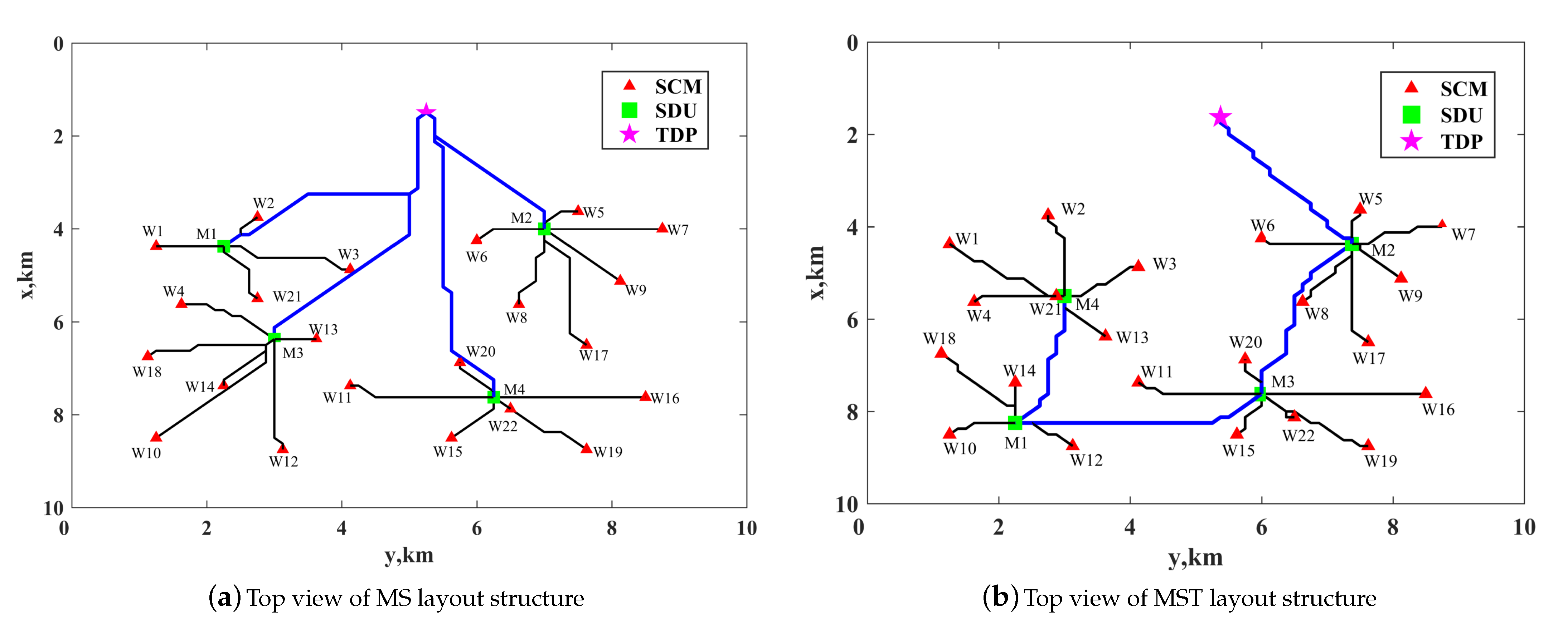
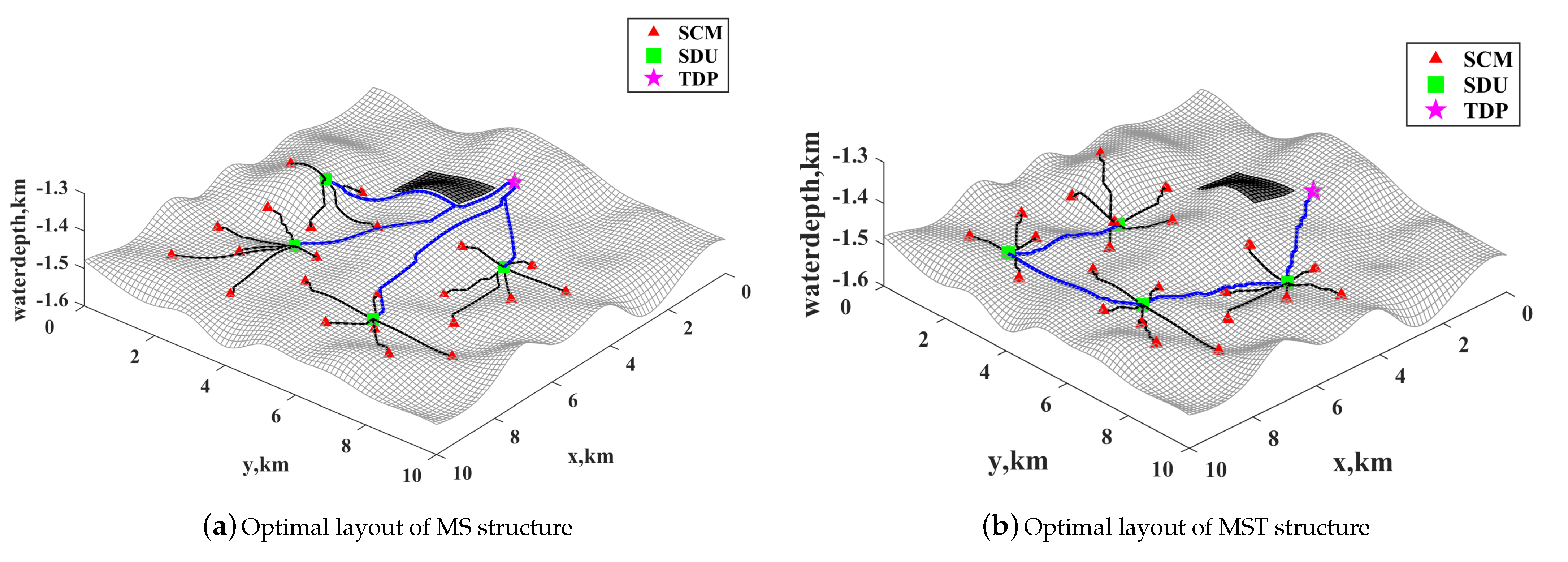
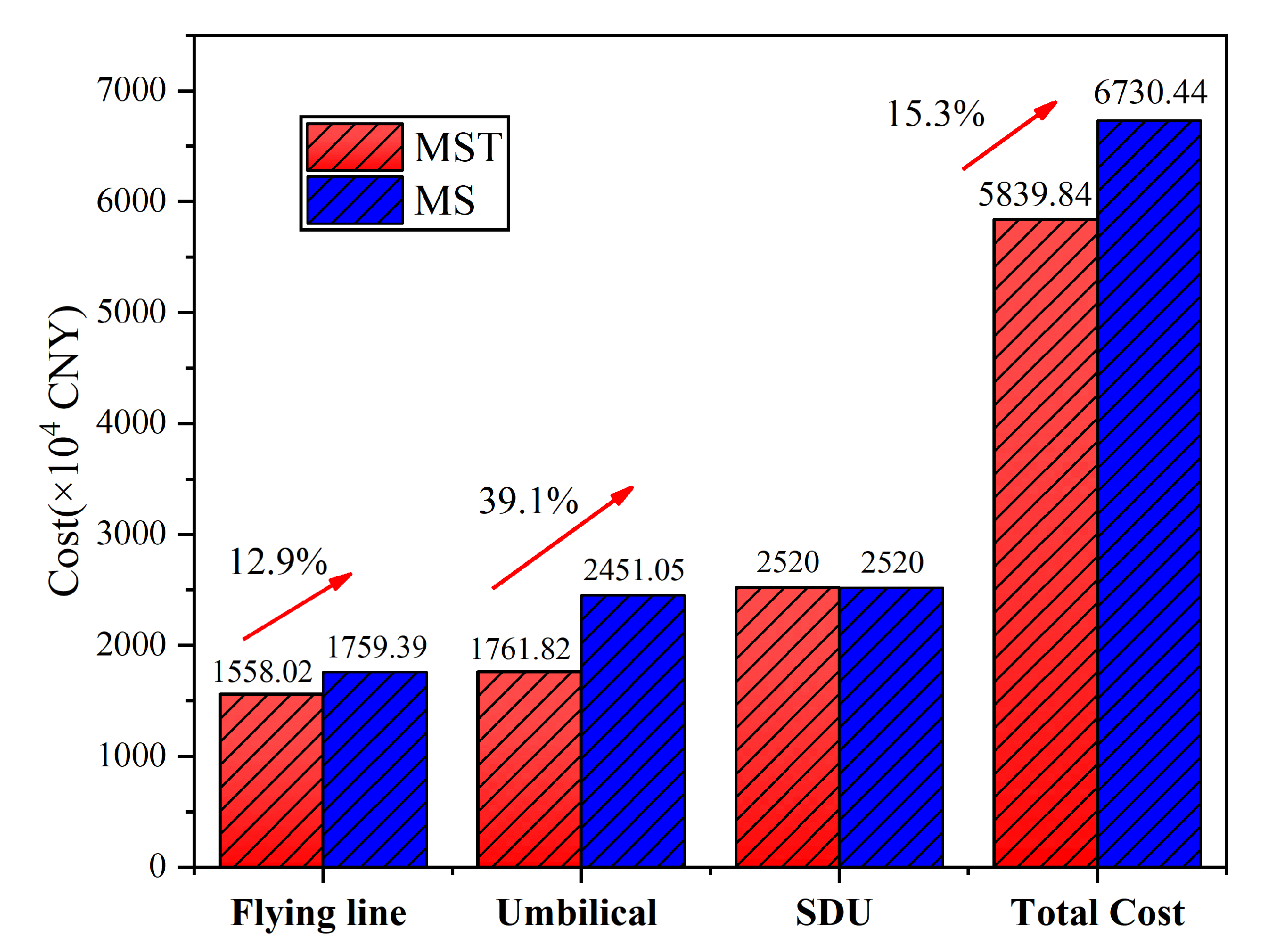
5. Case Study and Discussion

5.1. Case Study

In order to demonstrate the effectiveness of the optimization method, a subsea production control system with 22 SCMs was taken as an example. The system was applied in a deepwater field with water depth ranging from 1300 m to 1600 m. The digitally gridded seabed terrain and SCM distribution are shown in Figure 5, and the black part is the obstacle area. The SCMs are represented by red triangles, and their coordinate data are listed in

Table 2. Coordinate data of SCMs.

SCM Number	Coordinate (km)	SCM Number	Coordinate (km)
1	(4.375, 1.250, −1.444)	12	(8.750, 3.125, −1.506)
2	(3.750, 2.750, −1.490)	13	(6.375, 3.625, −1.502)
3	(4.875, 4.125, −1.475)	14	(7.375, 2.250, −1.494)
4	(5.625, 1.625, −1.485)	15	(8.500, 5.625, −1.494)
5	(3.625, 7.500, −1.504)	16	(7.625, 8.500, −1.513)
6	(4.250, 6.000, −1.481)	17	(6.500, 7.625, −1.514)
7	(4.000, 8.750, −1.506)	18	(6.750, 1.125, −1.503)
8	(5.625, 6.625, −1.520)	19	(8.750, 7.625, −1.487)
9	(5.125, 8.125, −1.496)	20	(6.875, 5.750, −1.498)
10	(8.500, 1.250, −1.488)	21	(5.500, 2.750, −1.499)
11	(7.375, 4.125, −1.499)	22	(5.500, 2.750, −1.499)

. The gridded seabed terrain is divided into $80\times 80$ nodes, and the length between two neighboring nodes is 125 m. To reduce the tension of the umbilical at the TDP, the horizontal distance, R, from the TDP to the FPSO is 650 m in Figure 1. In this work, there are two available types of SDU, each with a different maximum number of SCM connections. The types of available SDU, the basic parameters of the SDU, the number of optimized SDU, and the costs are listed in

Table 3. Available SDU types and parameters.

MAX SCM Number	Basic Cost (CNY ${10}^4$)	Additional Cost (CNY ${10}^4$)	Unit Price (CNY ${10}^4$)	Optimised Number	Total Cost (CNY ${10}^4$)
4	300	60	540	1	2520
6	300	60	660	3

.

After obtaining the number of SDUs, the problem dimension was determined for both layout structures. Too few particles promoted the algorithm to be trapped in local optimization, while too many particles slowed down the algorithm. For most optimization problems, the population size between 30 and 50 obtains a great solution [44]. Considering the complexity of the solution, the swarm size is thus set by 30 in this paper. Considering simplicity and efficiency, the values $w_{max}=0.9$ and $w_{min}=0.4$ are widely accepted in the literature [44]. In the literature, setting $c_1=c_2=2$ has been proposed as a generally acceptable setting for most problems [44]. In order to compare the final results of the two layout structures, the parameters are set the same. The algorithm parameters are listed in

Table 4. Main parameters of the AMPSO algorithm.

Problem Dimensions	Iteration Step	SwarmSize	${\mathit{w}}_{min}$	${\mathit{w}}_{max}$	${\mathit{c}}_1$	${\mathit{c}}_2$
13	200	30	0.4	0.9	2	2
18	200	30	0.4	0.9	2	2

.

The model is solved in MATLAB by applying the above parameters and the mentioned algorithms. Due to the complexity of the calculation, the positions of SDU and TDP are selected at the grid nodes of seabed terrain. The convergence curves of the hybrid algorithm for the functional pipeline cost for the MS and MST layout structure are shown in Figure 6. The x axis represents the iteration steps and the y axis represents the fitness value, which is the cost of the functional pipeline. The red line represents the optimal fitness curve and the blue dotted line represents the historical optimal average fitness curve. After approximately 50 iterations, the historical optimal average fitness curve and the current optimal fitness curve overlap, which indicates that the iterative process converges and obtains an optimal layout. The runtimes of the hybrid algorithm for MS and MST layout problems are 12,266.4 s and 15,453.4 s. Considering the swarm size and the number of nodes, the running time of the hybrid algorithm is acceptable.

Both layout structures satisfy all constraints after optimization with the proposed model and the hybrid algorithm. The subsea production control system controls the production of oil and gas, and thus the layout of the subsea production control system is carried out after the layout of the oil- and gas-gathering system is completed. In this work, the MS and MST layout structures of subsea production control system are optimized for the same oil and gas gathering system. Both these layout structures have independent mathematical models and corresponding optimization processes and methods, thus the two layouts can be independently configured. Figure 7 shows the top view of the optimal layout of the both layout structures for subsea production control system. Figure 8 shows the optimal layout in three-dimensional space. In Figure 7 and Figure 8, the red triangle represents the SCM, the green square represents the SDU, the pink star represents the TDP, the black lines are the flying lines connecting the SDU to the SCM and the blue lines are the umbilical. The specific information of the optimal layout for the MS and MST structures are shown in

Table 5. The specific information of the optimal layout for MS layout structure.

TDP Position (km)	SDU Position (km)	SCM Number	Umbilical Length (km)	Flying Line Length (km)	Functional Pipe Cost (CNY $\times {10}^4$)
(1.500, 5.250, −1.472)	(4.375, 2.250, −1.453)	W1	5.0725	1.0007	4210.44
		W2		0.8334
		W3		2.0843
		W21		1.3336
	(4.000, 7.000, −1.509)	W5	3.2253	0.7286
		W6		1.1039
		W7		1.7500
		W8		1.7804
		W9		1.5913
		W17		2.7590
	(6.375, 3.000, −1.497)	W4	5.8079	1.6863
		W10		2.8502
		W12		2.4270
		W13		0.6250
		W14		1.1307
		W18		2.0307
	(7.625, 6.250, −1.502)	W11	6.5397	2.2287
		W15		1.1339
		W16		2.2501
		W19		1.8413
		W20		0.9571
		W22		0.3536

and

Table 6. The specific information of the optimal layout for the MST layout structure.

TDP Position (km)	SDU Position (km)	Connection Relation 1	Flying Line Length (km)	Connection Relation 2	Umbilical Length (km)	Functional Pipe Cost ($\times {10}^4$ CNY)
(1.625, 5.375, −1.452)	(8.250, 2.250, −1.498)	M1-W10	1.1036	M1-M3	4.0090	3319.84
		M1-W12	1.0821
		M1-W14	0.8750
		M1-W18	2.0392
	(4.375, 7.375, −1.515)	M2-W5	0.8019	M2-FPSO	3.6522
		M2-W6	1.4273
		M2-W7	1.5304
		M2-W8	1.5607
		M2-W9	1.1341
		M2-W17	2.2286
	(7.625, 6.000, −1.499)	M3-W11	1.9787	M3-M2	3.8198
		M3-W15	1.0304
		M3-W16	2.5001
		M3-W19	2.0913
		M3-W20	0.8536
		M3-W22	0.7804
	(5.500, 3.000, −1.504)	M4-W1	2.2186	M4-M1	3.0609
		M4-W2	1.8538
		M4-W3	1.3843
		M4-W4	1.4274
		M4-W13	1.1339
		M4-W21	0.1250

. In Table 6, connection 1 represents the connection relationship between SDU and SCM and connection 2 represents the connection relationship between SDU and FPSO or SDU.

Figure 9 shows the overall comparison of the optimization results for the two layout structures. Due to the MST layout structure, the cost of the flying line and umbilical are 12.9% and 39.1% higher than the MS layout structure. The total cost is 15.3% higher. From the economic viewpoint, the subsea production control system of the MST layout structure is superior.

The suitable layout structure should be selected according to the practical subsea oilfield situation. Through the proposed optimization method and the model, the positions of the SDU and TDP, the number of SDU, the connection topology of functional pipelines and the functional pipeline routes are obtained. These results can be used for the pipeline route design, equipment installation and other subsequent work.

5.2. Discussion

5.2.1. Influence of Seabed Terrain

In order to compare the influence of the seabed terrain, the two layout structures are optimized assuming that the seabed is flat. The seabed terrain affects the undulation of the functional pipeline and thus affects the cost of the functional pipeline. The comparative results are shown in Figure 10, which indicates that the functional pipeline cost increases by 7.02% and 5.78% for the two layout structures. With the seabed terrain, the layout results are more realistic, making the cost estimation more reliable.

5.2.2. Optimization Algorithm

The AMPSO algorithm is used to determine the positions of the SDU and TDP, and the interconnection topology of functional pipe for two layout structures. The AMPSO algorithm has global search capability, as described in Section 3.1. This algorithm is efficient and can be conveniently realized, so it was selected to solve the problem. The A-star algorithm was applied to determine the pipeline route and the route was optimal. However, these two algorithms have several shortcomings. Due to the mutation operation, the AMPSO algorithm converges with many iterations. The A-star algorithm requires storing the route between the start points to every passed point until the target point is encountered. Thus, this algorithm takes up a large amount of storage space and has relatively low efficiency. In a more complex search environment, improved methods and other algorithms should be selected.

6. Conclusions

This paper proposes an integral optimization method to design the layout of subsea production control system in three-dimensional space. Furthermore, the layout optimization mathematical models for the MS and MST layout structure are established. Minimum total costs are defined as the objective function. Through the model, the numbers of SDU, the positions of the SDU and umbilical TDP, the pipe connection topology and the pipe routes can be determined for each layout structure. There were two key aspects considered in this paper. The first aspect is that the seabed terrain and obstacles are considered in the layout problem. The second aspect is that a hybrid algorithm combining AMPSO and A-star algorithms is applied to integrally optimize the interacting variables, which are the positions of the SDU and umbilical TDP, the pipe connection topology and the pipe routes. A subsea production control system with 22 SCMs and one FPSO is arranged for both layout structures to prove the practicality of the method. Two conclusions were acquired based on the case study. Firstly, compared with the MS and MST layout structures, the subsea production control system of the MST layout structure reduces the length of the functional pipeline, thus the MST layout structure has lower cost. Secondly, compared with the lack of effect from the seabed terrain, the cost of functional pipelines, respectively, increases by 7.02% and 5.78% for the MST and MS layout structure, therefore considering the seabed terrain constraint can provide a more reliable cost estimate.

When studying the layout of the subsea production control system in the future, this method can be applied to obtain an optimal layout scheme. However, the model proposed in this paper has several limitations. This article only focuses on reducing the construction cost of the subsea production control system. In fact, the layout is also affected by other factors, such as the reliability and stability of pipes and the flow assurance of hydraulic control signals. In order to make the model more practical, the above complex situations need to be studied. Furthermore, the intelligent optimization algorithm should be improved to enhance the solution efficiency in the future.

References

1. Kaiser, M.J. World offshore energy loss statistics. Energy Policy 2007, 35, 3496–3525. [Google Scholar] [CrossRef]
2. Herdeiro, M.; da Cunha, C.; Motta, B. Development of the Barracuda Furthermore, Caratinga Subsea Production System—An Overview. In Proceedings of the Offshore Technology Conference, Houston, TX, USA, 2–5 May 2005; pp. 1–12. [Google Scholar] [CrossRef]
3. Longo, C.E.; Neto, S.; Paula, M.; Lopes, F.; Godinho, C. Albacora Leste field-subsea production system development. In Proceedings of the Offshore Technology Conference, Houston, TX, USA, 1–4 May 2006; pp. 916–930. [Google Scholar] [CrossRef]
4. Lorenzatto, R.; Juiniti, R.; Gomes, J.; Martins, J. The Marlim Field Development: Strategies and Challenges. In Proceedings of the Offshore Technology Conference, Houston, TX, USA, 3–6 May 2004; pp. 1–9. [Google Scholar] [CrossRef]
5. Buckley, K.; Uehara, R. Subsea Concept Alternatives for Brazilian Pre-Salt Fields. In Proceedings of the Offshore Technology Conference in Brasil, Rio de Janeiro, Brazil, 24–26 October 2017; pp. 11–24. [Google Scholar] [CrossRef]
6. Duncan, T.; Braathen, B.I.; McCormack, N.; Stauble, M.; Campbell. One gulf reaching 50 billion boe and growing. In Proceedings of the Offshore Technology Conference, Houston, TX, USA, 30 April–3 May 2018; pp. 3584–3607. [CrossRef]
7. Beltrao, R. Cost reduction in deep water production systems. In Proceedings of the Offshore Technology Conference, Houston, TX, USA, 1–4 May 1995; pp. 11–24. [Google Scholar] [CrossRef]
8. Bai, Y.; Bai, Q. (Eds.) Overview of Subsea Engineering. In Subsea Engineering Handbook, 2nd ed.; Publishing House: Boston, MA, USA, 2019; pp. 3–22. [Google Scholar] [CrossRef]
9. Zuo, X.; Yue, Y.; Duan, Y.; Guo, L. An Overview of Subsea Production Control System. Mar. Eng. Equip. Technol. 2016, 3, 58–66. [Google Scholar]
10. Yasseri, S.F.; Bahai, H. Availability assessment of subsea distribution systems at the architectural level. Ocean Eng. 2018, 153, 399–411. [Google Scholar] [CrossRef]
11. Cui, Z.; Lin, H.; Wu, Y.; Wang, Y.; Feng, X. Optimization of Pipeline Network Layout for Multiple Heat Sources Distributed Energy Systems Considering Reliability Evaluation. Processes 2021, 9, 1308. [Google Scholar] [CrossRef]
12. Duan, Z.; Liao, Q.; Wu, M.; Zhang, H.; Liang, Y. Optimization of pipeline network structure of cbm fields considering three-dimensional geographical factors. In Proceedings of the 2016 11th International Pipeline Conference, Calgary, AB, Canada, 26–30 September 2016; pp. 1–12. [Google Scholar] [CrossRef]
13. Zhang, H.; Liang, Y.; Zhang, W.; Wang, B.; Yan, X.; Liao, Q. A unified MILP model for topological structure of production well gathering pipeline network. J. Pet. Sci. Eng. 2017, 152, 284–293. [Google Scholar] [CrossRef]
14. Zhang, H.; Liang, Y.; Ma, J.; Qian, C.; Yan, X. An MILP method for optimal offshore oilfield gathering system. Ocean Eng. 2017, 141, 25–34. [Google Scholar] [CrossRef]
15. Wu, Y.; Xu, S.; Zhao, H.; Wang, Y.; Feng, X. Coupling Layout Optimization of Key Plant and Industrial Area. Processes 2020, 8, 185. [Google Scholar] [CrossRef] [Green Version]
16. Wang, Y.; Wu, Y. A chemical industry area-wide layout design methodology for piping implementation. Chem. Eng. Res. Des. 2017, 118, 81–93. [Google Scholar] [CrossRef]
17. Rodrigues, H.; Prata, B.; Bonates, T. Integrated optimization model for location and sizing of offshore platforms and location of oil wells. J. Pet. Sci. Eng. 2016, 145, 734–741. [Google Scholar] [CrossRef] [Green Version]
18. Silva, L.; Guedes Soares, C. An integrated optimization of the floating and subsea layouts. Ocean Eng. 2019, 191, 106557. [Google Scholar] [CrossRef]
19. Wang, Y.; Duan, M.; Xu, M.; Wang, D.; Feng, W. A mathematical model for subsea wells partition in the layout of cluster manifolds. Appl. Ocean Res. 2012, 36, 26–35. [Google Scholar] [CrossRef]
20. Wang, Y.; Duan, M.; Feng, J.; Mao, D.; Xu, M.; Estefen, S.F. Modeling for the optimization of layout scenarios of cluster manifolds with pipeline end manifolds. Appl. Ocean Res. 2014, 46, 94–103. [Google Scholar] [CrossRef]
21. Wang, Y.; Wang, Q.; Zhang, A.; Qiu, W.; Duan, M.; Wang, Q. A new optimization algorithm for the layout design of a subsea production system. Ocean Eng. 2021, 232, 109072. [Google Scholar] [CrossRef]
22. Liu, H.; Gjersvik, T.B.; Faanes, A. Subsea field layout optimization (part II)–the location-allocation problem of manifolds. J. Pet. Sci. Eng. 2022, 208, 109273. [Google Scholar] [CrossRef]
23. Ribeiro, R.; Baioco, J.S.; Pires, B.S.L. Optimal design of submarine pipeline routes by genetic algorithm with different constraint handling techniques. Adv. Eng. Softw. 2014, 76, 110–124. [Google Scholar] [CrossRef]
24. Baioco, J.S.; Albrecht, C.H.; de Lima, B.S.L.P.; Jacob, B.P.; Rocha, D.M. Multi-Objective Optimization of Subsea Pipeline Routes in Shallow Waters. In Proceedings of the ASME 2017 36th International Conference on Offshore Mechanics and Arctic Engineering, Trondheim, Norway, 25–30 June 2017; pp. 11–15. [Google Scholar] [CrossRef]
25. Kang, J.Y.; Lee, B.S. Optimisation of pipeline route in the presence of obstacles based on a least cost path algorithm and laplacian smoothing. Int. J. Nav. Archit. Ocean Eng. 2017, 9, 492–498. [Google Scholar] [CrossRef]
26. Hong, C.; Estefen, S.F.; Lourenço, M.I.; Wang, Y. A nonlinear constrained optimization model for subsea pipe route selection on an undulating seabed with multiple obstacles. Ocean Eng. 2019, 186, 106088. [Google Scholar] [CrossRef]
27. Zhang, H.; Liang, Y.; Ma, J.; Shen, Y.; Yan, X.; Yuan, M. An improved PSO method for optimal design of subsea oil pipelines. Ocean Eng. 2017, 141, 154–163. [Google Scholar] [CrossRef]
28. Ruan, W.; Bai, Y.; Cheng, P. Static analysis of deepwater lazy-wave umbilical on elastic seabed. Ocean Eng. 2014, 91, 73–83. [Google Scholar] [CrossRef]
29. Bai, Y.; Bai, Q. (Eds.) Subsea Umbilical Systems. In Subsea Engineering Handbook, 2nd ed.; Publishing House: Boston, MA, USA, 2019; pp. 837–862. [Google Scholar] [CrossRef]
30. Yang, Z.; Yan, J.; Sævik, S.; Lu, Q.; Ye, N.; Chen, J.; Yue, Q. Integrated optimisation design of a dynamic umbilical based on an approximate model. Mar. Struct. 2021, 78, 102995. [Google Scholar] [CrossRef]
31. Rentschler, M.U.; Adam, F.; Chainho, P. Design optimization of dynamic inter-array cable systems for floating offshore wind turbines. Renew. Sustain. Energy Rev. 2019, 111, 622–635. [Google Scholar] [CrossRef]
32. Tan, Z.; Li, X.; Zhang, F. Design and research on suubsea production control system configuration. Autom. Petrochem. Ind. 2016, 52, 13–17. [Google Scholar]
33. Nasri, N.; Mnasri, S.; Val, T. 3D node deployment strategies prediction in wireless sensors network. Int. J. Electron. 2020, 107, 808–838. [Google Scholar] [CrossRef]
34. Mnasri, S.; Nasri, N.; Alrashidi, M.; van den Bossche, A.; Val, T. IoT networks 3D deployment using hybrid many-objective optimization algorithms. J. Heuristics 2020, 26, 663–709. [Google Scholar] [CrossRef]
35. Kennedy, J.; Eberhart, R. Particle swarm optimization. In Proceedings of the ICNN’95-International Conference on Neural Networks, Perth, WA, Australia, 27 November–1 December 1995; Volume 4, pp. 1942–1948. [Google Scholar] [CrossRef]
36. Yen, G.G.; Leong, W.F. A Multiobjective Particle Swarm Optimizer for Constrained Optimization. Int. J. Swarm. Intell. Res. 2011, 2, 1–23. [Google Scholar] [CrossRef]
37. Li, D.; Guo, W.; Lerch, A.; Li, Y.; Wang, L.; Wu, Q. An adaptive particle swarm optimizer with decoupled exploration and exploitation for large scale optimization. Swarm Evol. Comput. 2021, 60, 100789. [Google Scholar] [CrossRef]
38. Wang, S.; Li, Y.; Yang, H. Self-adaptive mutation differential evolution algorithm based on particle swarm optimization. Appl. Soft Comput. 2019, 81, 105496. [Google Scholar] [CrossRef]
39. Liang, H.; Kang, F. Adaptive mutation particle swarm algorithm with dynamic nonlinear changed inertia weight. Optik 2016, 127, 8036–8042. [Google Scholar] [CrossRef]
40. Yang, C.; Gu, L.; Gui, W. Particle Swarm Optimization Algorithm with Adaptive Mutation. Comput. Eng. 2008, 16, 188–190. [Google Scholar]
41. Hart, P.E.; Nilsson, N.J.; Raphael, B. A Formal Basis for the Heuristic Determination of Minimum Cost Paths. IEEE Trans. Syst. Sci. Cybern. 1968, 4, 100–107. [Google Scholar] [CrossRef]
42. Xiao, J.; Al-Muraikhi, A.; Qahtani, A.M. Automated route finding for production flowlines to minimize liquid inventory and pressure loss. In Proceedings of the SPE Annual Technical Conference and Exhibition, San Antonio, TX, USA, 24–27 September 2006; pp. 1–7. [Google Scholar] [CrossRef]
43. Ammar, A.; Bennaceur, H.; Châari, I.; Koubâa, A.; Alajlan, M. Relaxed Dijkstra and A* with Linear Complexity for Robot Path Planning Problems in Large-Scale Grid Environments. Soft Comput. 2016, 20, 4149–4171. [Google Scholar] [CrossRef]
44. Rezaee, A.; Jasni, J. Parameter selection in particle swarm optimisation: A survey. J. Exp. Theor. Artif. Intell. 2013, 25, 527–542. [Google Scholar] [CrossRef]
Figure 1. Simplified framework of subsea production control system.
Processes 09 01947 g001
Figure 2. Top view of two pipeline layout structures.
Processes 09 01947 g002
Figure 3. Pipe route overlaps and crossings.
Processes 09 01947 g003
Figure 4. The hybrid algorithm flow diagram of the integral optimization.
Processes 09 01947 g004
Figure 5. Seabed terrain and SCM distribution.
Processes 09 01947 g005
Figure 6. Convergence curves of the hybrid optimization algorithm with two layout structures.
Processes 09 01947 g006
Figure 7. Top view of the optimal layout for the two layout structures.
Processes 09 01947 g007
Figure 8. Optimal layout in three-dimensional space for the two layout structures.
Processes 09 01947 g008
Figure 9. Overall comparison of the optimization results for the two layout structures.
Processes 09 01947 g009
Figure 10. Comparison of the total pipeline cost with and without seabed terrain.
Processes 09 01947 g010