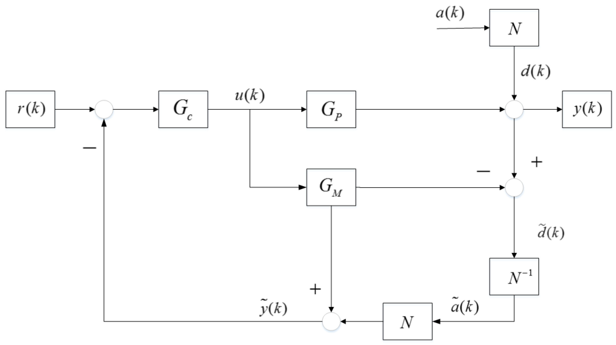
The Wood and Berry distillation is a typical binary column one that is obtained from and designed for a methanol water mixture MIMO system. This distillation model has been widely used in many literatures as a benchmark of MIMO control scheme for deep study, further comparison and engineering practice. The closed loop mainly contains four sections, the two manipulated variables (MV)
and
, the two controlled variables (CV)
and
, The
transfer function
as well as the disturbance noise signals
and
. The relations of these symbols form the formula below.
The MPC controller was selected as the brain of this MIMO closed loop system and implemented in the process. The prediction horizon of MPC values 100 and the control horizon is equal to 10, which are the same as those in document [
26] by comparison. The weighting factors of control variables (CV), the manipulated variables (MV), and the set-points of two outputs are
,
and
in
Table 2, respectively. The variances of two white noises
are equal to 1.0, with discretized disturbance noise formula expression
.
4.1.1. Causality in No Model Plant Mismatch Mode
In this section, the Granger causality method was carried out under the condition that there was no model plant mismatch problem in the system. The data from operating mode that worked well could be gathered as a data base benchmark for further fault diagnosis.
Considering the Equation (
17), the Granger causality was started from self regression of the variables.
in different channels should be regressed so that a basic understanding of systematical data could be obtained and compared later.
The character “R(u1,0),AR(d1,1–20)” in
Figure 3 means that this causality analysis is only interrelated to the auto regression of
in first closed loop without any other factors affecting the analysis. The change from “R(u1,0)” to “R(u1,1)” implied that one step Granger regression was implemented to detect the causality from manipulated variable output
to the detected data sequence
in first channel.
The red line is merely corresponding to the variances of auto-regression mode. The blue curve describes just one step causality regression of and the green one gives a description of two step causality regressions.
Every part of four pictures in
Figure 3 consists of three kinds of curves. The red-point curve implies the result of causality. The value of regression variance descends with the increase of auto-regression length, which is equivalent to the model order selection in system identification. Higher order can depict more details of the whole system but enhance the difficulty of controlling. It is necessary and reasonable to choose a proper size, like AIC criterion. As the nominal model is known to us, too high order is costly and unnecessary when it is greater than a convergent one. The biggest length of experiment is 20, which is enough to reveal the uniform convergence of auto-regression.
“Times” means the length of regression or auto regression coefficients, namely, the result of model order selection.
In view of the information in
Table 3, the variance of white noise
and that of
were equal to 1, which played as a simplified noise benchmark in theory. But in real industrial, the variance is never just right the same as the set point value and always changing with data fluctuations. Sometimes the variance will be a little higher or lower than the designed one. The fluctuated value converges on the theoretical variance.
The Equations (
26) and (
32) suggest that the variance of auto regression should be equal to that of pure white noise in each channel if no MPM occurred in this loop. However, Granger causality is a kind of regression methods that is based on statistical approaches so that overfitting of data is existing from start to finish. on the other hand, a lot of uncertainties in white noise make slight phenomenons. The first one is that the mean value of white noise is converging to zero but the real value is fluctuating nearby zero. The second one is that the variance is also converging and fluctuating around the theoretical value that equals 1 as designed.
From Theorem 4, the raise of model orders results in monotone increasing of Granger index. If curves do not coincide, such monotone increasing will cause regression curves to approach the benchmark line. Hence, model order should not be too high.
Figure 3 displayed the problems that statistical characteristics of
and
were approximately equal to theoretical value 1. In consideration of that the concept of overfitting and statistical fluctuation are inevitable, the results of variance could be accepted.
The model orders ware embodied in the lengths of auto regression about
and
. Too large order would lead to overfitting problems. Both of the two kind variances were gradually declining on the whole due to overfitting. Other than system identification, model orders were not so important as the causality. And to avoid the statistical interference in Granger analysis, upper and lower limits were adopted. If the causality regression results of
or
are within the limit lines, then the variance of
will be regarded as equal with
. The expectation of
is almost the same with
so that
.
Similarly, it can be obtained that
4.1.2. Causality Compared with Decussation in Mismatch
The decussation method consists of two techniques, correlation analysis method between the input and the disturbance (CAID) and model quality index (MQI). Both methods can help to locate the MPM positions after coordination.
The process model varied from
to
.
Obviously, MPM occurred in Equation (
92) and
got mismatched in the system.
The data correlation between u1, the manipulated variable in first channel named
and ds, the estimated noise in CAID algorithm, was below zero and its absolute value declined from 0.7071 to 0.4255 in
Table 4 and
Table 5. However, the correlation between u2 and ds also reduced. Besides, The MQI(2) was 0.9697 and similar to 1.0, which was as ideal as theoretical one.
The red and the blue curve that got coincidence in
Figure 4a,b implies it may have no causality because the regression of
dedicates no variance decrease to fault analyses. The scopes of variances are also below 1.0 close to 0.97 as the same condition of auto regression overfitting. Even the green curves describe some causality, and the scopes of variances are next to convergence value.
The
Figure 4a,b reveals that
in the first channel got no mismatch, which was under the same condition with that in
Figure 3. The bottom pictures showed some differences and suggested the mismatch problems.
The sequence of is still composed of two parts. The first one is the disturbance noise as well as its transfer function . The other is the mismatched part, . Thus, the autoregression of would get larger than its theoretical values.
The variance of was above 1.0 in the beginning and got remarkable declines after Granger causality analysis.
The bottom two pictures (c)(d) in
Figure 4 indicate that model plant mismatch exists in second channel but it is uncertain for the user to judge where the fault position is or whether two channels mismatch occurs together. To overcome these shortcomings, the assistant model of noise
is introduced here.
The Equation (
93) showed that causality in the second loop was larger than zero and the existence of mismatch was ensured.
A hint from
Figure 5 implies that only model from u1 to the second channel mismatched. The average value in
Figure 4 about data benchmark of the first five variances is 1.0122 and the mean value of causality is 0.9770. The decline of variance was caused by Granger regressions.
Due to model mismatch in , the Granger index changed with this kind of interference. At this moment, consisted of two parts, the mismatch part as well as the noise part.
If got mismatched, the Granger causality index would reduce after regression analysis from to . Before regression method adopted, the sequence contained the mismatched information. After regression, the mismatched signal was extracted so that the left sequence contained nothing on and .
The top picture in
Figure 5 reveals a better identification. The first coefficient of noise model in
is 0.9. The maximum value in upper picture is almost 0.9, and the left coefficients are near to zero at the same time. The lower picture got a worse identification for misunderstanding. It was because that no matter
or
devoted nothing on mismatch that the extraction got wrong shapes. Considering
increased more space for regression, the overfitting occurred.
The
Figure 5a depicts a series of curves fluctuating slightly and converging to the theoretical values as noise transfer function. Better convergence effects than picture
Figure 5b are because the regression of
extracted most causality from the channel
towards
. The
Figure 5b got bounding but only the facts that top line is equal to 0.9 as noise model set and the other parameters remains to be zero, embody correct regression. It was because the channel from
towards
devoted no causality to the MIMO systems that the regression in this channel did not know the mismatch condition. the causality algorithm forced it to overfit, and the parameters which are not near zero were not essential but once existed, would get over-fitted.
The convergence features of coefficients indicate the correct regression result from to and help to locate the channel i to j. Better convergence implies more reasonable regression and the less variance indicates the more significant Granger causality index. It is the real mismatched channel that reflects the occurrence of MPM so that the extraction of this channel information with regression technique can help to get a stable causality calculations. The index can quantify the fluctuations of parameters in .
Considering
, the regression effects
were in
Figure 6 and
Figure 7. All the parameters in
Figure 6 were less than
and its variances were less than
, too. A better regression revealed the mismatch was from
to
, which showed that
had a MPM problem.
Among the 20 coefficients in
Figure 7, eight of them were larger than
and became over-limited. No mismatch plus regression method made this overfitting.
With the help of Equation (
94), the location was finished and the mismatch position was from
.
4.1.3. Causality Compared with Decussation in and Mismatches
In this section, two mismatches occurred in different channels. Besides, the mismatch positions in model parameters were also diverse.
got its model mismatch in gain parts while
became distinct in its denominator coefficient.
The decussation method showed that the significant declines of MQI(1) and CAID(u2,ds) pointed to the mismatch in , but bad effects on CAID(u1,ds) with good results of MQI(2) could not located the mismatch in .
CAID shows a negative influence of mismatches in both row channels. MQI(1) and CAID(u1,ds) locates an incorrect mismatch from
to
in
Table 6. The reason is obvious, for data in MIMO system will get mutual interference. The information from
and
mismatches conducted to
link and change the statistical characteristics, which caused erroneous judgment.
and mismatches had not been detected while the were wrongly judged. Besides, MQI(2) was seeming to normal but a little abnormal. If the judgment was correct, the mismatch would be missed. If the judgment was incorrect, then the four channels would get mismatched, which did not happen.
These suggest that decussation based on statistical correlation should be inaccurate, although it is a momentous means in analyzing the control loops.
Causalities in
Figure 8 reveal all the channels got notable decreases in variances. It was possible that at least two mismatches existing in the closed loop system.
The variance of auto regression of
was 1.1 in
Figure 8, suggesting that mismatch brought about worse Granger regression. And the variance of
still got increased than before from 0.9939 to1.03.
Assistant model parameters would be,
and the locations of mismatch from
to
and another from
to
were ensured in view of Formula (
98).
The
Figure 9b,c shows a better convergence feature, which indicates two significant regression results from
to
and from
to
. Regression method extracts almost all mismatch information so that the left parameters of noise models are correct. The first coefficient of
is converging to 0.8 and the second one to 0.9, which are consistent with Equation (
88).


