Acceptance Sampling Plans from Life Tests Based on Percentiles of New Weibull–Pareto Distribution with Application to Breaking Stress of Carbon Fibers Data

Abstract

In this paper, acceptance sampling plans (ASPs) are proposed for the new Weibull-Pareto distribution (NWPD) percentiles assuming truncated life tests at a pre-determined time. The minimum sample sizes essential to assert the specified percentile are calculated for a given consumer’s risk. The operating characteristic function values of the developed ASPs and producer’s risk are provided. A real data set related to the breaking stress of carbon fibers data are presented for illustration.

1. Introduction

The quality of a product is important to long-serving customers, while at the same time, owners or producers of the product are interested in saving costs and time in the production process. These objectives have encouraged researchers in the field to find a tool in order to maintain the quality of products lots. Acceptance sampling plans are well known in industry to emphasize the acceptability of a lot based on a random sample selected from the product. Based on this sample, the consumer can accept or reject the lot. The process of the acceptance sampling plan (ASP) operates by first obtaining the minimum ample size that is important to emphasize a certain percentile or average life when the life test is terminated at a pre-specified time. These types of tests are called truncated lifetime tests.

Different types of ASP are known to practitioners as the single ASP, double ASP, group ASP, multiple ASP as well as other methods. Details regarding these types can be found in previous papers: single ASP to the exponential distribution by [1], the three-parameter Lindley distribution [2], ASP for the exponentiated Fréchet distribution [3], double ASP for the NWPD is suggested by [4], single ASP for the NWPD is proposed by [5], three parameters Kappa distribution [6], single ASP for the generalized Rayleigh distribution [7], single ASP for the weighted exponential distribution [8], ASP for length-biased weighted Lomax distribution [9,10] single ASP for generalized exponential distribution [9,11] for the Akash distribution. These works have considered the mean as a quality parameter. Further works include ASP for log-logistic distribution [12], for single ASP under exponentiated inverse Rayleigh distribution [10,13] for ASP based on generalized inverted exponential distribution see [14].

For ASP based on model percentiles, single ASP for percentiles under the linear failure rate distribution [15], ASP for percentiles under the inverse Rayleigh distribution [16], the Birnbaum Saunders distribution for percentiles [17], for Log-Logistic distribution for percentiles [18,19] for the ASP percentile under Marshall–Olkin extended Lomax distribution.

The structure of the paper is as follows. In Section 2, the NWPD is introduced. Section 3 describes the suggested ASP under the NWPD. Section 4 provides Illustrative examples for the real data set. Finally, our conclusions are summarized in Section 5.

2. The NWPD

The NWPD is introduced by [20] as a new continuous lifetime distribution to be more flexible in fitting real data in various fields. Ref. [21] suggested the exponentiated NWPD as a modification of the NWPD. Ref. [22] used the ranked set sampling to estimate the parameters of the NWPD. The distribution function of the NWPD has the form

$$F(x;\alpha ,\theta ,\eta )=1-e^{-\alpha {\left(\frac{x}{\theta }\right)}^{\eta }},\hspace{1em}x>0,\eta ,\theta ,\alpha >0,$$

(1)

with a probability density function provided by

$$f(x;\alpha ,\theta ,\eta )=\frac{\alpha \eta }{{\theta }^{\eta }}{x}^{\eta -1}{e}^{-\alpha {\left(\frac{x}{\theta }\right)}^{\eta }},$$

(2)

The mean and the variance of the model, respectively, are

$$\begin{array}{c}E\left(X\right)=\theta {\alpha }^{-\frac{1}{\eta }}\mathsf{\Gamma }\left[\frac{\eta +1}{\eta }\right]\\ \mathrm{and}Var\left(X\right)=2\theta {\alpha }^{-\frac{2}{\eta }}\mathsf{\Gamma }\left[\frac{\eta +2}{\eta }\right]-{\left[\theta {\alpha }^{-\frac{1}{\eta }}\mathsf{\Gamma }\left(\frac{\eta +1}{\eta }\right)\right]}^2\end{array}$$

(3)

The NWPD has a hazard rate function and mode at $x=x_0$, respectively, provided by

$$H(x)=\frac{\alpha \eta }{{\theta }^{\eta }}{x}^{\eta -1}\mathrm{and}{x}_0=\theta {\left\{\frac{\eta -1}{\alpha \eta }\right\}}^{\frac{1}{\eta }}$$

The 100q-th percentile of the NWPD is

$$t_q=\theta {\left(\frac{1}{\alpha }ln\left(\frac{1}{1-q}\right)\right)}^{\frac{1}{\eta }}$$

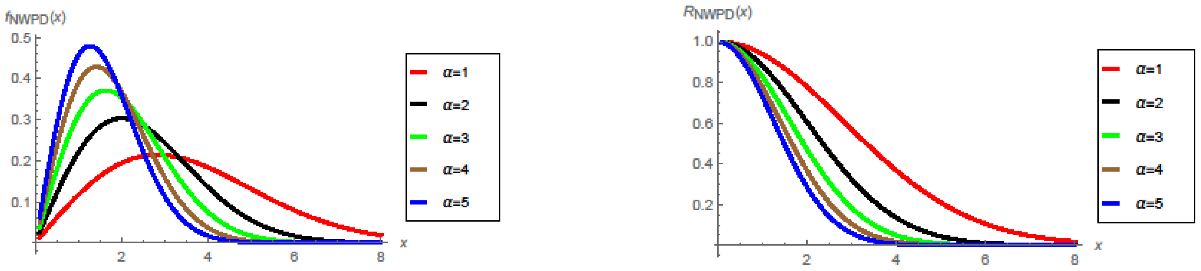
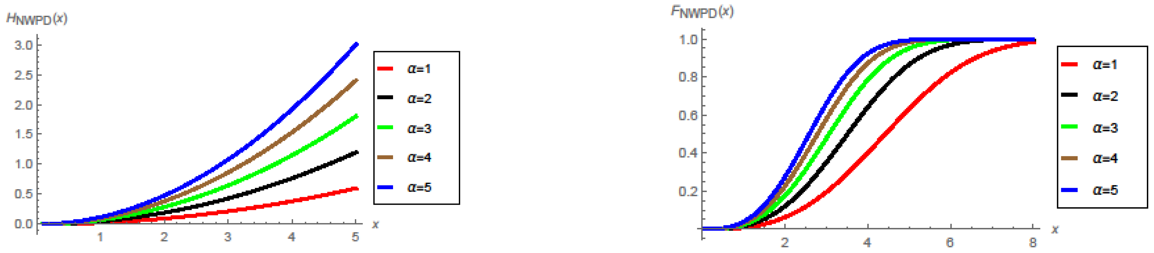
In Figure 1, we presented the plot of pdf and reliability functions of the NWPD for some selected parameters. Additionally, in Figure 2, the hazard function and the distribution function of the NWPD are offered. It is clear that the model is skewed to the right with decreasing reliability function for the selected parameter values. In Figure 2, it is noted that the hazard function increases for $\eta =2,\theta =4$ as $\alpha =1,2,3,4,5$.

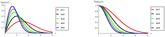
Figure 1. The pdf and reliability function of the NWPD with $\eta =2,\theta =4$.

Figure 2. The hazard and distribution functions of the NWPD with $\eta =2,\theta =4$.

3. The Suggested ASP

Assume that the life test is scheduled to be t, and c is the maximum number of admissible bad lots to accept the lot, with at least $p^{\ast }$ being the probability of rejecting a bad lot. The truncated life test ASPs for percentile is to maintain the minimum sample size n for a specified acceptance number c provided that the consumer’s risk (which is the probability of accepting a bad lot) doesn’t exceed $1-p^{\ast }$. A bad lot that is the true is in the 100qth percentile, while $t_q$ is less than the identified percentile $t_q^0$. Thus, the probability of rejecting a bad lot with $t_q^{}<t_q^0$ is at least equal to $p^{\ast }$. In this sense, the parameters of the offered sampling plan are $\left(n,c,t_q/t_q^0\right)$ with a probability $p^{\ast }$.

3.1. Minimum Sample Size

For a fixed $p^{\ast }$ where $p^{\ast }\in \left(0,1\right)$, the suggested ASPs can be characterized by $\left(n,c,t/t_q^0\right)$, assuming that the lot size is adequately large so that the binomial distribution can be employed. The smallest positive sample size n needed to assert that $t_q>t_q^0$ should satisfy the inequality

$${\displaystyle \sum _{i=0}^c\left(\begin{array}{c}n\\ i\end{array}\right)}{p}^i{(1-p)}^{n-i}\le 1-p^{\ast }$$

(4)

where $p=F(t;{\delta }_0)$ is the probability of a failure observed through the time t given that a determined $100q\mathrm{th}$ percentile for lifetime $t_q^0$ which depends only on ${\delta }_0=t/t_q^0$.

$F\left(t;\delta \right)$ is a non-decreasing function of $\delta ,$ since $\partial F(t;\delta )/\partial \delta >0$. Therefore, $F\left(t;\delta \right)<F\left(t;{\delta }_0\right)\leftrightarrow \delta \le {\delta }_0$, which is equivalently

$$F\left(t;\delta \right)\le F\left(t;{\delta }_0\right)\leftrightarrow t_q\le t_q^0$$

(5)

The smallest sample size n that satisfies (3) can be obtained for any given q, ${\delta }_0=t/t_q^0$, $p^{\ast }$, $\theta ,\alpha ,\eta$. For illustration, the required smallest sample sizes are obtained for q = 0.1 $t/t_q^0=$ 0.628, 0.942, 1.257, 1.571, 2.356, 3.141, 3.927, 4.712, $p^{\ast }=$ 0.75, 0.9, 0.95, 0.99 and $c=0,1,2,\dots ,10$. The results are shown in Table 1 for $\eta =2.793$ and $\alpha =1.011$ under the NWPD. Further, the minimum sample size values are presented in Table 2 for $\eta =2$ and $\alpha =2$.

Table 1. Minimum sample sizes necessary to assure the percentile q = 0.1 life of a product to exceed a given $t_{0.1}^0$ with $\eta =2.793$ and $\alpha =1.011$ for the NWPD.

${\mathit{p}}^{\ast }$	c	${\mathit{\delta }}_{0.1}^0$
		0.628	0.942	1.257	1.571	2.356	3.141	3.927	4.712
0.75	0	49	16	7	4	2	1	1	1
	1	95	31	15	8	3	2	2	2
	2	138	45	21	12	5	3	3	3
	3	180	59	28	16	7	5	4	4
	4	221	73	34	19	8	6	5	5
	5	261	86	40	23	10	7	6	6
	6	301	100	46	27	11	8	7	7
	7	341	113	53	30	13	9	8	8
	8	380	126	59	34	15	10	9	9
	9	420	139	65	37	16	11	10	10
	10	459	152	71	41	18	12	11	11
0.9	0	81	26	12	7	2	1	1	1
	1	136	45	21	11	4	3	2	2
	2	187	61	28	16	6	4	3	3
	3	235	77	36	20	8	5	4	4
	4	281	92	43	24	10	6	5	5
	5	326	107	50	28	11	7	6	6
	6	370	122	56	32	13	9	7	7
	7	414	136	63	36	15	10	8	8
	8	457	150	70	40	16	11	9	9
	9	499	164	76	43	18	12	10	10
	10	542	178	83	47	20	13	11	11
0.95	0	105	34	16	9	3	2	1	1
	1	166	54	25	14	5	3	2	2
	2	221	72	33	18	7	4	3	3
	3	272	89	41	23	9	5	4	4
	4	321	105	48	27	11	7	5	5
	5	369	121	56	31	13	8	6	6
	6	416	136	63	35	14	9	8	7
	7	462	151	70	40	16	10	9	8
	8	507	166	77	44	18	11	10	9
	9	552	181	84	47	19	13	11	10
	10	596	196	91	51	21	14	12	11
0.99	0	161	52	24	13	4	2	1	1
	1	232	75	34	19	7	4	3	2
	2	294	96	44	24	9	5	4	3
	3	352	115	52	29	11	6	5	4
	4	406	133	61	34	13	8	6	5
	5	459	150	69	38	15	9	7	6
	6	511	167	77	43	17	10	8	7
	7	561	183	84	47	18	11	9	8
	8	610	200	92	51	20	13	10	9
	9	659	216	99	56	22	14	11	10
	10	707	231	107	60	24	15	12	11

Table 2. Minimum sample sizes necessary to assure the percentile q = 0.1 life of a product to exceed a given $t_{0.1}^0$ with $\eta =2$ and $\alpha =2$ for the NWPD.

${\mathit{p}}^{\ast }$	c	${\mathit{\delta }}_{0.1}^0$
		0.628	0.942	1.257	1.571	2.356	3.141	3.927	4.712
0.75	0	34	15	9	6	3	2	1	1
	1	66	30	17	11	6	4	3	2
	2	96	43	25	17	8	5	4	4
	3	125	57	33	22	11	7	6	5
	4	154	70	40	27	13	9	7	6
	5	182	82	48	32	16	11	8	7
	6	209	95	55	37	18	12	10	8
	7	237	108	62	41	21	14	11	9
	8	264	120	69	46	23	16	12	10
	9	292	132	77	51	26	17	13	12
	10	319	145	84	56	28	19	15	13
0.9	0	56	25	14	9	4	3	2	1
	1	95	43	24	16	8	5	4	3
	2	130	58	33	22	11	7	5	4
	3	163	73	42	28	14	9	6	5
	4	195	88	51	33	16	10	8	7
	5	226	102	59	39	19	12	9	8
	6	257	116	67	44	22	14	11	9
	7	287	130	75	49	24	16	12	10
	8	317	144	83	55	27	18	13	11
	9	347	157	90	60	30	19	15	13
	10	376	170	98	65	32	21	16	14
0.95	0	73	33	18	12	6	3	2	2
	1	115	52	30	19	9	6	4	3
	2	153	69	39	26	12	8	6	4
	3	189	85	49	32	15	10	7	6
	4	223	100	58	38	18	12	9	7
	5	256	115	66	44	21	13	10	8
	6	289	130	75	49	24	15	11	9
	7	320	145	83	55	27	17	13	11
	8	352	159	91	60	30	19	14	12
	9	383	173	99	66	32	21	16	13
	10	414	187	108	71	35	23	17	14
0.99	0	111	50	28	18	8	5	3	2
	1	161	72	41	27	12	7	5	4
	2	204	91	52	34	16	10	7	5
	3	244	109	62	41	19	12	8	7
	4	282	127	72	47	22	14	10	8
	5	318	143	82	53	26	16	12	9
	6	354	159	91	60	29	18	13	11
	7	389	175	100	66	32	20	15	12
	8	423	191	109	72	35	22	16	13
	9	457	206	118	77	37	24	17	14
	10	490	221	127	83	40	26	19	16

3.2. OC of the Sampling Plan $\left(n,c,t/t_q^0\right)$

For the ASP $\left(n,c,t/t_q^0\right)$, the OC function of the sampling plan is the probability of acceptance of a lot. The OC is defined as

$$L(p)={\displaystyle \sum _{i=0}^c\left(\begin{array}{c}n\\ i\end{array}\right)}{p}^i{(1-p)}^{n-i}$$

(6)

where $p=F(t;\delta )$. It is of interest that $p=F(t;\delta )$ can be utilized as a function of $\delta =t/t_q$. Hence, $p=F\left(\frac{t}{t_q^0}\frac{1}{d_q}\right),d_q=\frac{t_q}{t_q^0}$. With reference to Equation (6), the values of the OC as a function of $d_q=\frac{t_q}{t_q^0}$ can be calculated for the sampling plan $\left(n,c=2,\frac{t}{t_q^0}\right)$ with the model parameter values. Table 3 is devoted to the OC values for the sampling plan $\left(n,c=2,t/t_{0.1}^0\right)$ when $\eta =2.793$ and $\alpha =1.011$ for the NWPD, and in Table 4 for $\eta =2$ and $\alpha =2$.

Table 3. OC values of sampling plans of $c=6$, for a given $p^{\ast }$ with $\eta =2.793$ and $\alpha =1.011$ for the NWPD.

${\mathit{p}}^{\ast }$	${\mathit{\delta }}_{0.1}^0$	n	${\mathit{d}}_{0.1}^0$
			2	4	6	8	10	12
0.75	0.628	301	0.999701	1	1	1	1	1
	0.942	100	0.999683	1	1	1	1	1
	1.257	46	0.999700	1	1	1	1	1
	1.571	27	0.999626	1	1	1	1	1
	2.356	11	0.999629	1	1	1	1	1
	3.141	8	0.998381	1	1	1	1	1
	3.927	7	0.992162	1	1	1	1	1
	4.712	7	0.929527	0.999998	1	1	1	1
0.9	0.628	370	0.998996	1	1	1	1	1
	0.942	122	0.998960	1	1	1	1	1
	1.257	56	0.998983	1	1	1	1	1
	1.571	32	0.998874	1	1	1	1	1
	2.356	13	0.998549	1	1	1	1	1
	3.141	9	0.994680	1	1	1	1	1
	3.927	7	0.992162	1	1	1	1	1
	4.712	7	0.929527	0.999998	1	1	1	1
0.95	0.628	416	0.998049	1	1	1	1	1
	0.942	136	0.998057	1	1	1	1	1
	1.257	63	0.997956	1	1	1	1	1
	1.571	35	0.998040	1	1	1	1	1
	2.356	14	0.997481	1	1	1	1	1
	3.141	9	0.994680	1	1	1	1	1
	3.927	8	0.964743	1	1	1	1	1
	4.712	7	0.929527	0.999998	1	1	1	1
0.99	0.628	511	0.994005	1	1	1	1	1
	0.942	167	0.993995	1	1	1	1	1
	1.257	77	0.993688	1	1	1	1	1
	1.571	43	0.993472	1	1	1	1	1
	2.356	17	0.990642	1	1	1	1	1
	3.141	10	0.987026	1	1	1	1	1
	3.927	8	0.964743	1	1	1	1	1
	4.712	7	0.929527	0.999998	1	1	1	1

Table 4. OC values of sampling plans of $c=2$, for a given p* with $\eta =2$ and $\alpha =2$ for the NWPD.

${\mathit{p}}^{\ast }$	${\mathit{\delta }}_{0.1}^0$	n	${\mathit{d}}_{0.1}^0$
			2	4	6	8	10	12
0.75	0.628	96	0.922106	0.997918	0.999798	0.999963	0.99999	0.999997
	0.942	43	0.923079	0.997949	0.999801	0.999963	0.99999	0.999997
	1.257	25	0.920043	0.997849	0.999791	0.999961	0.99999	0.999997
	1.571	17	0.912496	0.997595	0.999765	0.999957	0.999988	0.999996
	2.356	8	0.916982	0.997740	0.999780	0.999959	0.999989	0.999996
	3.141	5	0.917525	0.997740	0.999779	0.999959	0.999989	0.999996
	3.927	4	0.888453	0.996659	0.999668	0.999938	0.999984	0.999994
	4.712	4	0.768052	0.990960	0.999051	0.99982	0.999951	0.999984
0.9	0.628	130	0.847796	0.995115	0.999508	0.999908	0.999975	0.999992
	0.942	58	0.849659	0.995194	0.999516	0.999910	0.999976	0.999992
	1.257	33	0.849863	0.995202	0.999517	0.999910	0.999976	0.999992
	1.571	22	0.842178	0.994871	0.999482	0.999903	0.999974	0.999991
	2.356	11	0.819956	0.993858	0.999373	0.999882	0.999968	0.999989
	3.141	7	0.798989	0.992813	0.99926	0.999861	0.999963	0.999987
	3.927	5	0.789398	0.992250	0.999197	0.999848	0.999959	0.999986
	4.712	4	0.768052	0.990960	0.999051	0.999820	0.999951	0.999984
0.95	0.628	153	0.788780	0.992353	0.999211	0.999851	0.999960	0.999986
	0.942	69	0.786140	0.992217	0.999196	0.999848	0.999959	0.999986
	1.257	39	0.788257	0.992325	0.999207	0.999851	0.999960	0.999986
	1.571	26	0.777140	0.991745	0.999144	0.999838	0.999957	0.999985
	2.356	12	0.782827	0.992028	0.999175	0.999844	0.999958	0.999986
	3.141	8	0.730352	0.989036	0.998841	0.999780	0.999940	0.99998
	3.927	6	0.679417	0.985610	0.998446	0.999702	0.999919	0.999973
	4.712	4	0.768052	0.990960	0.999051	0.999820	0.999951	0.999984
0.99	0.628	204	0.647266	0.983466	0.998200	0.999654	0.999906	0.999968
	0.942	91	0.648696	0.983574	0.998212	0.999657	0.999907	0.999968
	1.257	52	0.643657	0.983189	0.998167	0.999648	0.999904	0.999967
	1.571	34	0.637692	0.982724	0.998112	0.999637	0.999901	0.999966
	2.356	16	0.625914	0.981766	0.997998	0.999614	0.999895	0.999964
	3.141	10	0.589807	0.978632	0.997620	0.999539	0.999874	0.999957
	3.927	7	0.569516	0.976613	0.997370	0.999489	0.999860	0.999952
	4.712	5	0.606321	0.979689	0.997739	0.999562	0.999881	0.999959

3.3. Producer’s Risk

The producer’s risk is the probability of rejecting the lot if $t_q>t_q^0$. For a given value of the producer’s risk, say $\varphi$, the researchers were interested in determining the value of $d_q$ to assert that the producer’s risk is less than or equal to $\varphi$ when the $\left(n,c,t/t_q^{}\right)$ is developed at a specified $p^{\ast }$. Therefore, we aimed to achieve the smallest value of $d_q$ satisfying $L(p)\ge 1-\varphi$. In this case,

$$P(\mathrm{Rejecting}\mathrm{a}\mathrm{lot})={\displaystyle \sum _{i=c+1}^n\left(\begin{array}{c}n\\ i\end{array}\right)}{p}^i{(1-p)}^{n-i}$$

(7)

Table 5 shows the minimum ratios of $d_{0.1}$ for the acceptability of a lot under $\varphi =0.05$ when $\eta =2.793$ and $\alpha =1.011$ for the NWPD and in Table 6, the ratio values show when for $\eta =2$ and $\alpha =2$.

Table 5. Minimum ratio of $d_{0.1}^0$ for the acceptability of a lot with producer’s risk 0.05 with $\eta =2.793$ and $\alpha =1.011$ for the NWPD.

${\mathit{p}}^{\ast }$	c	$\mathit{t}/{\mathit{t}}_{\mathit{q}}^0$
		0.628	0.942	1.257	1.571	2.356	3.141	3.927	4.712
0.75	0	3.2738	3.2893	3.2647	3.3394	3.9074	4.0645	5.0815	6.0973
	1	2.0711	2.0722	2.1184	2.0896	2.0993	2.2951	2.8694	3.4430
	2	1.7554	1.7532	1.7635	1.7779	1.8411	1.8538	2.3177	2.7810
	3	1.6058	1.6055	1.6229	1.6329	1.7162	1.9154	2.0581	2.4695
	4	1.5156	1.5187	1.5230	1.5159	1.5466	1.7479	1.9031	2.2835
	5	1.4536	1.4547	1.4569	1.4650	1.5149	1.6351	1.798	2.1574
	6	1.4092	1.4141	1.4096	1.4280	1.4234	1.5529	1.7211	2.0652
	7	1.3755	1.3787	1.3839	1.3810	1.4144	1.4899	1.6618	1.9940
	8	1.3477	1.3509	1.3546	1.3608	1.4059	1.4397	1.6143	1.9370
	9	1.3263	1.3283	1.3309	1.3296	1.3531	1.3985	1.5752	1.8900
	10	1.3075	1.3096	1.3113	1.3172	1.3512	1.3640	1.5422	1.8504
0.9	0	3.9193	3.9138	3.9597	4.0803	3.9074	4.0645	5.0815	6.0973
	1	2.3564	2.3724	2.3983	2.3581	2.3776	2.7987	2.8694	3.4430
	2	1.9585	1.9592	1.9639	1.9878	2.0011	2.1973	2.3177	2.7810
	3	1.7679	1.7700	1.7840	1.7827	1.8272	1.9154	2.0581	2.4695
	4	1.6528	1.6534	1.6646	1.6636	1.7252	1.7479	1.9031	2.2835
	5	1.5752	1.5765	1.5858	1.5850	1.5893	1.6351	1.7980	2.1574
	6	1.5183	1.5215	1.5194	1.5289	1.5516	1.6865	1.7211	2.0652
	7	1.4754	1.4762	1.4784	1.4867	1.5226	1.6116	1.6618	1.9940
	8	1.4406	1.4406	1.4463	1.4535	1.4542	1.5520	1.6143	1.9370
	9	1.4116	1.4120	1.4132	1.4136	1.4404	1.5032	1.5752	1.8900
	10	1.3885	1.3883	1.3924	1.3927	1.4287	1.4623	1.5422	1.8504
0.95	0	4.3009	4.3084	4.3892	4.4644	4.5179	5.2093	5.0815	6.0973
	1	2.5313	2.5341	2.5565	2.5806	2.6058	2.7987	2.8694	3.4430
	2	2.0798	2.0809	2.0872	2.0792	2.1400	2.1973	2.3177	2.7810
	3	1.8635	1.8660	1.8727	1.8816	1.9266	1.9154	2.0581	2.4695
	4	1.7341	1.7352	1.7347	1.7419	1.8025	1.9187	1.9031	2.2835
	5	1.6472	1.6491	1.6549	1.6498	1.7204	1.7842	1.7980	2.1574
	6	1.5838	1.5834	1.5885	1.5841	1.6085	1.6865	1.9415	2.0652
	7	1.5350	1.5340	1.5386	1.5502	1.5714	1.6116	1.8628	1.9940
	8	1.4957	1.4953	1.4995	1.5098	1.5421	1.5520	1.8000	1.9370
	9	1.4640	1.4641	1.4680	1.4649	1.4804	1.5913	1.7485	1.8900
	10	1.4370	1.4384	1.4420	1.4392	1.4644	1.5451	1.7053	1.8504
0.99	0	5.0121	5.0162	5.0750	5.0926	5.0081	5.2093	5.0815	6.0973
	1	2.8545	2.8531	2.8596	2.8892	2.9763	3.1698	3.4990	3.4430
	2	2.3045	2.3096	2.3202	2.3174	2.3764	2.4546	2.7472	2.7810
	3	2.0446	2.0482	2.0450	2.0555	2.1009	2.1185	2.3947	2.4695
	4	1.8871	1.8913	1.8965	1.9034	1.9407	2.0619	2.1852	2.2835
	5	1.7819	1.7836	1.7891	1.7853	1.8349	1.9096	2.0442	2.1574
	6	1.7057	1.7068	1.7126	1.7165	1.7595	1.7988	1.9415	2.0652
	7	1.6463	1.6457	1.6477	1.6512	1.6611	1.7140	1.8628	1.9940
	8	1.5988	1.6009	1.6034	1.6000	1.6213	1.7298	1.8000	1.9370
	9	1.5606	1.5621	1.5619	1.5698	1.5891	1.6690	1.7485	1.8900
	10	1.5283	1.5278	1.5330	1.5349	1.5625	1.6181	1.7053	1.8504

Table 6. Minimum ratio of $d_{0.1}^0$ for the acceptability of a lot with producer’s risk 0.05 with $\eta =2$ and $\alpha =2$ for the NWPD.

${\mathit{p}}^{\ast }$	c	$\mathit{t}/{\mathit{t}}_{\mathit{q}}^0$
		0.628	0.942	1.257	1.571	2.356	3.141	3.927	4.712
0.75	0	5.2482	5.2289	5.4047	5.5152	5.8486	6.3664	5.6283	6.7533
	1	2.7675	2.7857	2.7796	2.7702	3.0016	3.1813	3.3426	3.0402
	2	2.1972	2.1912	2.2098	2.2540	2.2283	2.2259	2.3843	2.8609
	3	1.9380	1.9486	1.9583	1.9734	2.0076	2.0178	2.2656	2.3616
	4	1.7905	1.7962	1.7911	1.8146	1.797	1.8949	1.9730	2.0783
	5	1.6895	1.6863	1.7018	1.7115	1.7286	1.8125	1.7826	1.8934
	6	1.6141	1.6178	1.6225	1.6385	1.6237	1.6568	1.803	1.7619
	7	1.5612	1.5664	1.5633	1.5630	1.5934	1.6262	1.6854	1.6629
	8	1.5169	1.5196	1.5173	1.5231	1.5278	1.6011	1.5935	1.5852
	9	1.4839	1.4820	1.4907	1.4908	1.5121	1.5156	1.5193	1.6837
	10	1.4543	1.4564	1.4593	1.4641	1.4659	1.5048	1.5551	1.6201
0.9	0	6.7354	6.7505	6.7408	6.7548	6.7533	7.7972	7.9595	6.7533
	1	3.3242	3.3438	3.3176	3.3669	3.5089	3.6156	3.9774	4.0107
	2	2.5604	2.5528	2.5520	2.5831	2.669	2.7462	2.7829	2.8609
	3	2.2162	2.2118	2.2209	2.2445	2.3072	2.3716	2.2656	2.3616
	4	2.0176	2.0200	2.0343	2.0214	2.0317	2.0327	2.1815	2.3673
	5	1.8853	1.8867	1.8967	1.9045	1.9146	1.9219	1.9599	2.1389
	6	1.7924	1.7931	1.8003	1.8000	1.8319	1.8433	1.9428	1.9771
	7	1.7202	1.7235	1.7286	1.7225	1.7276	1.7842	1.8105	1.8556
	8	1.6643	1.6695	1.6730	1.6791	1.6847	1.7379	1.7072	1.7605
	9	1.6196	1.6209	1.6191	1.6294	1.6500	1.6415	1.7202	1.8231
	10	1.5808	1.5812	1.5835	1.5887	1.5915	1.6168	1.6445	1.7495
0.95	0	7.6901	7.7557	7.6433	7.7997	8.2711	7.7972	7.9595	9.5506
	1	3.6591	3.6809	3.7172	3.6786	3.7366	4.0018	3.9774	4.0107
	2	2.7793	2.7883	2.7811	2.8188	2.8003	2.9708	3.1263	2.8609
	3	2.388	2.3902	2.4053	2.4083	2.3986	2.5288	2.5228	2.7185
	4	2.159	2.1564	2.1749	2.1787	2.1737	2.2815	2.3691	2.3673
	5	2.0078	2.0062	2.0109	2.0311	2.0289	2.0248	2.1194	2.1389
	6	1.9019	1.901	1.9096	1.9069	1.9273	1.9290	1.9428	1.9771
	7	1.8176	1.8229	1.8229	1.8329	1.8517	1.8576	1.9257	2.0223
	8	1.7549	1.7567	1.7558	1.7598	1.7931	1.8020	1.8118	1.9120
	9	1.7026	1.7039	1.7023	1.7155	1.7147	1.7574	1.8100	1.8231
	10	1.6598	1.6607	1.6666	1.6665	1.6793	1.7207	1.7279	1.7495
0.99	0	9.4827	9.5466	9.5329	9.5526	9.5506	10.0662	9.7484	9.5506
	1	4.3322	4.3372	4.3557	4.4032	4.3481	4.3532	4.5203	4.7725
	2	3.2119	3.2078	3.2221	3.2389	3.2725	3.3741	3.4334	3.3392
	3	2.7157	2.7121	2.7148	2.7412	2.7334	2.8161	2.7535	3.0271
	4	2.4302	2.4355	2.4318	2.4363	2.4326	2.5045	2.5413	2.6176
	5	2.2399	2.2420	2.2502	2.2409	2.2893	2.3046	2.4028	2.3516
	6	2.1070	2.1069	2.1113	2.1232	2.1469	2.1647	2.1914	2.3312
	7	2.0060	2.0069	2.0085	2.0196	2.0415	2.0611	2.1344	2.1724
	8	1.9257	1.9296	1.9291	1.9396	1.9600	1.9809	2.0017	2.0484
	9	1.8616	1.8633	1.8658	1.8631	1.8663	1.9170	1.8948	1.9485
	10	1.8075	1.8092	1.8140	1.8122	1.8159	1.86470	1.8814	1.9732

Based on the results presented in Table 1 and Table 2, we can see that the values of minimum sample sizes depend on the values of the distribution parameters.

4. Illustrative Examples

In this section, the performance of the suggested ASPs based on percentiles of the NWPD is investigated based on a real data set. The data set represents the breaking stress of carbon fibers (in Gba), which has already been studied by [23]. The observations are: 0.39, 0.81, 0.85, 0.98, 1.08, 1.12, 1.17, 1.18, 1.22, 1.25, 1.36, 1.41, 1.47, 1.57, 1.57, 1.59, 1.59, 1.61, 1.61, 1.69, 1.69, 1.71, 1.73, 1.80, 1.84, 1.84, 1.87, 1.89, 1.92, 2.00, 2.03, 2.03, 2.05, 2.12, 2.17, 2.17, 2.17, 2.35, 2.38, 2.41, 2.43, 2.48, 2.48, 2.50, 2.53, 2.55, 2.55, 2.56, 2.59, 2.67, 2.73, 2.74, 2.76, 2.77, 2.79, 2.81, 2.81, 2.82, 2.83, 2.85, 2.87, 2.88, 2.93, 2.95, 2.96, 2.97, 2.97, 3.09, 3.11, 3.11, 3.15, 3.15, 3.19, 3.19, 3.22, 3.22, 3.27, 3.28, 3.31, 3.31, 3.33, 3.39, 3.39, 3.51, 3.56, 3.60, 3.65, 3.68, 3.68, 3.68, 3.70, 3.75, 4.20, 4.38, 4.42, 4.70, 4.90, 4.91, 5.08, 5.56. Table 7 presents the summary statistics of the data.

Table 7. Descriptive statistics of the carbon fibers data.

n	Mean	Sd	Median	Kurtosis	Skewness	Min	Max
100	2.62	1.01	2.7	0.04	0.36	0.39	5.56

The distribution parameters were estimated using the maximum likelihood estimation (MLE) method and maximized value of the log likelihood function based on the considered model were obtained. We used the criteria of Bayesian information (BIC), Hannan–Quinn information (HQIC), Akaike information (AIC), and consistent Akaike information (CAIC). The Kolmogorov–Smirnov (KS), and Anderson–Darling (AD) statistics were obtained. The fitting results are presented in Table 8.

Table 8. The BIC, AIC, HQIC, CAIC, AD, W, KS, and −2LL for the carbon fibers data.

BIC	AIC	HQIC	CAIC	AD	W	−2LL	KS	p-Value
296.8741	289.0586	292.2217	289.3086	0.41581	0.06227	141.5293	0.06049	0.85780

The MLE of the NWPD parameters are $\widehat{\alpha }=1.0113$, $\widehat{\theta }=2.95557$ and $\widehat{\eta }=2.79286$. The values of the criteria show that the NWPD fits well the carbon fibers data.

Assume that the researcher intends to emphasize that the true unknown 10th percentile lifetime for the time breaking stress of carbon fibers is at least 1000 h with probability $p^{\ast }=0.75$, and assume that the life test will be terminated at t= 942 h, leading to the ratio $\delta =t/t_{0.1}^0=0.942$. Hence, for the acceptance number c = 6 and confidence level $p^{\ast }=0.75$, the corresponding sample size in Table 1 is $n=100$. Therefore, the ASP for the 10th percentile of NWPD should be $\left(n,c,t/t_{0.1}^0\right)=\left(100,6,0.942\right)$. Based on the breaking stress of carbon fibers data, the researcher must make a decision about whether to reject or accept the lot. If a sample of 100 runoff amounts is selected, the lot is accepted when no more than six failures occur before breaking stress of carbon fibers 0.942. Based on to this plan, the breaking stress of carbon fibers can be accepted because there are only three failures before the termination of the time.

The OC function values for the new ASP $\left(n,c,t/t_{0.1}^0\right)=\left(100,6,0.942\right)$ when $p^{\ast }=0.75$ under the NWPD with $\eta =2.793$ and $\alpha =1.011$ from Table 2 are:

$t_{0.1}^{}/t_{0.1}^0$	2	4	6	8	10	12
OC	0.999683	1	1	1	1	1

This implies that if the true 10th percentile is two times the specified percentile life $(t_{0.1}^{}/t_{0.1}^0=2),$ the producer’s risk is about 0.000317, and the producer’s risk is zero when $t_{0.1}^{}\ge t_{0.1}^0=4$.

It can be seen from Table 3, which provides the values of $d_{0.1}$ for various choices of the acceptance c and $t/t_{0.1}^0$, that the producer’s risk should not more than 0.05. Thus, for the ASP $\left(n,c,t/t_{0.1}^0\right)=\left(100,6,0.942\right)$ and $p^{\ast }=0.75$, the table entry is 1.4141. This means that the product should have a 10th percentile life of at least 1.4141 times the necessary 10th percentile lifetime based on the ASP $\left(n,c,t/t_{0.1}^0\right)=\left(100,6,0.942\right)$ such that the product is accepted with a probability of 0.95 or more.

5. Conclusions

This paper suggests new ASPs for the percentiles of the NWPD based on truncated lifetime tests. Tables of minimum sample sizes, the operating characteristic function values as well as the associated producer’s risks are presented for selected values of the model parameters. An application example of real data is provided for illustration. It can be concluded that the developed ASP can be easily implemented for practitioners. The group acceptance sampling plans based on the NWPD can be considered for future research.

References

- Sobel, M.; Tischendrof, J.A. Acceptance sampling with new life test objectives. In Proceedings of the Fifth National Symposium Reliability and Quality Control, Philadelphia, PA, USA, 12 January 1959; pp. 108–118. [Google Scholar]
- Al-Omari, A.I.; Al-Nasser, A.D.; Ciavolino, E. Economic design of acceptance sampling plans for truncated life tests using three-parameter Lindley distribution. J. Mod. Appl. Stat. Methods 2020, 18, 1–15. [Google Scholar] [CrossRef]
- Al-Nasser, A.D.; Al-Omari, A.I. Acceptance sampling plan based on truncated life tests for exponentiated fréchet distribution. J. Stat. Manag. Syst. 2013, 16, 13–24. [Google Scholar] [CrossRef]
- Al-Omari, A.I.; Al-Nasser, A.D.; Gogah, F.S. Double acceptance sampling plan for time truncated life tests based on new Weibull-Pareto distribution. Electron. J. Appl. Stat. Anal. 2016, 9, 520–529. [Google Scholar]
- Al-Omari, A.I.; Santiago, A.; Sautto, J.M.; Bouza, C.N. New Weibull-Pareto distribution in acceptance sampling plans based on truncated life tests. Am. J. Math. Stat. 2018, 8, 144–150. [Google Scholar]
- Al-Omari, A.I. Acceptance Sampling Plan Based on Truncated Life Tests for Three Parameter Kappa Distribution. Econ. Qual. Control 2014, 29, 53–62. [Google Scholar] [CrossRef]
- Tsai, T.-R.; Wu, S.-J. Acceptance sampling based on truncated life tests for generalized Rayleigh distribution. J. Appl. Stat. 2006, 33, 595–600. [Google Scholar] [CrossRef]
- Gui, W.; Aslam, M. Acceptance sampling plans based on truncated life tests for weighted exponential distribution. Commun. Stat.-Simul. Comput. 2015, 46, 2138–2151. [Google Scholar] [CrossRef]
- Al-Omari, A.I.; Almanjahie, I.M.; Kravchuk, O. Acceptance Sampling Plans with Truncated Life Tests for the Length-biased Weighted Lomax Distribution. Comput. Mater. Contin. 2021, 67, 285–301. [Google Scholar] [CrossRef]
- Aslam, M.; Kundu, D.; Ahmad, M. Time truncated acceptance sampling plans for generalized exponential distribution. J. Appl. Stat. 2010, 37, 555–566. [Google Scholar] [CrossRef]
- Al-Omari, A.I.F.; Koyuncu, N.; Alanzi, A.R.A. New Acceptance Sampling Plans Based on Truncated Life Tests for Akash Distribution with an Application to Electric Carts Data. IEEE Access 2020, 8, 201393–201403. [Google Scholar] [CrossRef]
- Kantam, R.R.L.; Rosaiah, K.; Rao, G.S. Acceptance sampling based on life tests: Log-logistic model. J. Appl. Stat. 2001, 28, 121–128. [Google Scholar] [CrossRef]
- Sriramachandran and Palanivel. Acceptance sampling plan from truncated life tests based on exponentiated inverse Rayleigh distribution. Am. J. Math. Manag. Sci. 2014, 33, 20–35. [Google Scholar]
- Al-Omari, A.I. Time truncated acceptance sampling plans for generalized inverted exponential distribution. Electron. J. Appl. Stat. Anal. 2015, 8, 1–12. [Google Scholar] [CrossRef]
- Rao, B.S.; Priya, M.C.; Kantam, R.R.L. Acceptance Sampling Plans for Percentiles Assuming the Linear Failure Rate Distribution. Econ. Qual. Control 2014, 29, 1–9. [Google Scholar] [CrossRef]
- Rao, B.S.; Kantam, R.R.L.; Rosaiah, K.; Reddy, P. Acceptance sampling plans for percentiles based on the inverse Rayleigh distribution. Electron. J. Appl. Stat. Anal. 2012, 5, 164–177. [Google Scholar]
- Lio, Y.L.; Tsai, T.-R.; Wu, S.-J. Acceptance sampling plan based on the truncated life test in the Birnbaum Saunders distribution for percentiles. Comm. Statist. Simul. Comput. 2009, 39, 119–136. [Google Scholar] [CrossRef]
- Lio, Y.; Tsai, T.-R.; Wu, S.-J. Acceptance sampling plans from truncated life tests based on the Burr type XII percentiles. J. Chin. Inst. Ind. Eng. 2010, 27, 270–280. [Google Scholar] [CrossRef]
- Rao, G.S.; Ghitany, M.E.; Kantam, R.R.L. Marshall–Olkin extended Lomax distribution: An economic reliability test plan. Int. J. Appl. Math. 2009, 22, 139–148. [Google Scholar]
- Nasiru, S.; Luguterah, A. The New Weibull-Pareto Distribution. Pak. J. Stat. Oper. Res. 2015, 11, 103–114. [Google Scholar] [CrossRef] [Green Version]
- Al-Omari, A.I.; Al-khazaleh, A.; Al-khazaleh, M. Exponentiated new Weibull-Pareto distribution. Rev. Investig. Oper. 2019, 40, 165–175. [Google Scholar]
- Samuh, M.H.; Al-Omari, A.I.; Koyuncu, N. Estimation of the parameters of the new Weibull-Pareto distribution using ranked set sampling. Statistica 2020, 80, 103–123. [Google Scholar]
- Andrews, D.F.; Herzberg, A.M. Data: A Collection of Problems from Many Fields for the Student and Research Worker; Springer Series in Statistics: New York, NY, USA, 1985. [Google Scholar]
Publisher’s Note: MDPI stays neutral with regard to jurisdictional claims in published maps and institutional affiliations. |
© 2021 by the authors. Licensee MDPI, Basel, Switzerland. This article is an open access article distributed under the terms and conditions of the Creative Commons Attribution (CC BY) license (https://creativecommons.org/licenses/by/4.0/).