Abstract
In this paper, the Nonlinear Auto-Regressive with exogenous inputs (NARX) model with parameters of interest for design (NARX-M-for-D), where the design parameter of the system is connected to the coefficients of the NARX model by a predefined polynomial function is studied. For the NARX-M-for-D of nonlinear systems, in practice, to predict the output by design parameter values are often difficult due to the uncertain relationship between the design parameter and the coefficients of the NARX model. To solve this issue and conduct the analysis and design, an improved algorithm, defined as the Weighted Extended Forward Orthogonal Regression (WEFOR), is proposed. Firstly, the initial NARX-M-for-D is obtained through the traditional Extended Forward Orthogonal Regression (EFOR) algorithm. Then a weight matrix is introduced to modify the polynomial functions with respect to the design parameter, and then an improved model, which is referred to as the final NARX-M-for-D is established. The genetic algorithm (GA) is used for deriving the weight matrix by minimizing the normalized mean square error (NMSE) over the data sets corresponding to the design parameter values used for modeling and first prediction. Finally, both the numerical and experimental studies are conducted to demonstrate the application of the WEFOR algorithm. The results indicate that the final NARX-M-for-D can accurately predict the system output of a nonlinear system. The new algorithm is expected to provide a reliable model for dynamic analysis and design of the nonlinear system.
1. Introduction
For the nonlinear systems, in general, the conventional dynamic modeling methods are often difficult or even impossible to obtain the motion equations describing the dynamical characteristics due to the uncertainty, time variability, and complexity [1,2]. An alternative approach to this issue is the data-driven modeling method known as system identification, which can be used to establish the numerical model of a nonlinear system by the input and output data sets. The Volterra model [3,4], some modern Volterra series approaches [5,6], and Hammerstein–Wiener model [7,8,9] have been widely used for representing the numerical representation of the nonlinear system. In the past years, the Nonlinear Auto-Regressive with exogenous inputs (NARX) model, which was introduced in 1985 [10,11], was widely used for establishing the nonlinear system models for prediction and analysis due to the convenience (see [12,13,14,15]). Among the numerous related model classes and neural network models, the NARX model is commonly adopted in many real-world cases, and this model is an expansion of past exogenous inputs and outputs. The identification algorithms developed based on NARX models have generally proven efficient for a wide range of nonlinear systems. Compared with neural network models, which have strong fitting ability, the NARX model is more convenient and can provide an explicit model structure to facilitate analysis and design [16]. However, the NARX model cannot represent the Common Model Structure (CMS) of the system and provide insight into the effect of design parameters on system response [17].
In recent years, researchers have looked for a modeling framework that involves design parameters to characterize better the dynamic behavior of the underlying system with different parameter values. The NARX model with parameters of interest for design (NARX-M-for-D) provides an effective solution to this issue, which based on the NARX model and connects the design parameter to the coefficients of the NARX model by a polynomial function [18]. The critical tasks in identification the NARX-M-for-D include detecting the CMS, estimating the associated coefficients, and establishing the function of the coefficients of the NARX model with respect to the design parameter [19]. To obtain the CMS and build a parsimonious model, Wei et al. [17] proposed the Extended Forward Orthogonal Regression (EFOR) algorithm, moreover, the Average Approximate Minimum Description Length (AAMDL) criterion is introduced to determine the total number of model terms. Incorrect model structure [20,21] can be obtained due to the overlapped information by using the EFOR algorithm, the Iterative EFOR (IEFOR) algorithm proposed by Liu et al. [19] can be used to overcome this issue. The IEFOR is developed based on the idea of the iterative Orthogonal Forward Regression (iOFR) algorithm, where the optimal model is obtained by iteration [22]. However, the relationship between the design parameter and the coefficients of the NARX model are predefined as a power-form polynomial function in the above research. For the nonlinear systems, in practice, to predict the coefficients of the NARX model by design parameter values and a predefined function may not reveal the system output accurately. Although the previous studies provide the methods to obtain the CMS, no reports have been found to consider the nonlinear relation between the design parameter values and system output in the process of predicting the system output.
To overcome the issue above, in this paper, an algorithm defined as the Weighted EFOR (WEFOR) is proposed to establish the NARX-M-for-D of a nonlinear system. The weight matrix is introduced to modify the coefficients polynomial functions. The first step of the identification process is similar to the idea of other improved methods for the identification of NARX-M-for-D, such as the IEFOR algorithm [19], the initial NARX-M-for-D is obtained based on the EFOR algorithm. Consequently, the polynomial functions of the coefficients of NARX models with respect to the design parameters are modified by introducing a weight matrix, and then an improved model referred to as the final NARX-M-for-D is obtained. The genetic algorithm (GA) [23] is used for deriving the weight matrix by minimizing the normalized mean square error (NMSE) over the training data sets corresponding to the design parameter values used for modeling and first prediction. The proposed algorithm can establish a reliable model for dynamic analysis and design of the nonlinear system. A key novelty of the WEFOR algorithm is that for the first time, the modeling process considers the uncertain relationship between the coefficients of the NARX model and design parameter.
The organization of the paper is as follows: Section 2 describes the NARX-M-for-D. In Section 3, the traditional identification algorithm known as the EFOR is introduced, and then the WEFOR algorithm is proposed to identify the final NARX-M-for-D. In Section 4, a NARX system is proposed as an illustrative case to show the effectiveness of the new algorithm, and then an experimental case is demonstrated by using a cylinder with a bolted joint. Finally, Section 5 draws the conclusions.
2. Modeling Framework—The NARX-M-for-D
It has been reported that the CMS with the design parameter can be represented by the following polynomial function [19,24]:
where is an unknown nonlinear function. and are system input and output variables of the system under the kth design parameter value, respectively. nu and ny are the maximum lags of the system input and output variables, respectively, n = nu + ny. l is the nonlinear degree order of function . are the coefficients of NARX model under the kth design parameter value. is the vector formed by the design parameter, . K is the number of design parameter values. e(t) represents the noise variable. (k = 1,2,…,K, m = 1,2,…,n) represent the delayed system input and output terms, which can be expressed as [19]:
Assume that the input and output variables of a Single-Input and Single-Output (SISO) system under K different design parameter values have been obtained, the nonlinear dynamic parametrical model with K different cases of design parameter properties can be obtained, which can be written as [25]:
where are the CMS with K sets of coefficients, which need to be identified from model dictionaries. It is worth mentioning that when K = 1, Models (1) and (3) are traditional NARX models [19].
To illustrate the model explicitly, the NARX-M-for-D can often be expressed in a linear regression function as [17]:
where are model terms made of delayed system input and output variables; represent the kth set of coefficients corresponding to the kth design parameter value; M is the number of candidate model terms in the predictor vectors, which can be derived by:
Remark 1: Considering the input variables are impossible to keep the same in practice, the framework of the NARX-M-for-D described in this section denotes the system input under different design parameter values by subscript k, and make the difference with Multi-Input and Multi-Output (MIMO) system. It is worth mentioning that, to emphasize the feasibility of modeling method, the noise is assumed to be white noise and not shown in the following.
3. The Weighted EFOR (WEFOR) Algorithm
Due to the uncertain and nonlinear relation between the design parameter and output of the nonlinear system, to predict the coefficients of the NARX model by design parameter values and a predefined polynomial function cannot reveal the behaviors of a nonlinear system accurately. To overcome this issue, in this section, the WEFOR algorithm is proposed, where the initial NARX-M-for-D is established based on the traditional EFOR algorithm, and then a weight matrix is introduced to modify the predefined polynomial function. The weight matrix is derived using the GA by minimizing the NMSE of all the data sets corresponding to the design parameter values used for modeling and first prediction. And then the improved model, which referred to as the final NARX-M-for-D is obtained by pre-multiplying the right side of the predefined function by the matrix. The details are as follows.
3.1. Traditional EFOR Algorithm
The EFOR algorithm is applied to obtain the CMS of a nonlinear system, determine the functional relationship between design parameter and coefficient of NARX models by using the Least Squares (LS) algorithm, and then the dynamic parametrical model can be obtained, which referred as the initial NARX-M-for-D. The EFOR algorithm is introduced as follows [19,24]:
Step 1: Orthogonalization of the models
Assuming that the NARX models under K parameter values have been obtained by using the FROLS algorithm [2,16], Model (4) can be rewritten as a matrix form:
where is system output under the kth design parameter value; is regression matrix made of the candidate model terms, ; and is the vector formed by coefficients of the kth NARX model, .
To minimize the predicting error, the regression matrix needs to be orthogonalized [25]. The orthogonalization can be done by using the Gram–Schmidt algorithm [22], and then Model (6) can be represented as:
where is the orthogonal matrix formed by the orthogonal vectors ; is the matrix of coefficients corresponding to , . and can be derived by Equations (8) and (9), respectively.
where <·,·> represents the inner product.
Step 2: The common model structure detection
The EFOR algorithm selects the common model terms in a stepwise manner based on the significance of all the model terms, which is measured by the index named Average Error Reduction Ratio (AERR). The formula to calculate the AERR can be written as follows [17]:
where the subscript m denotes the mth regressor in the candidate pool of orthogonal model terms.
The ith AERR in the searching process is defined as:
Specify a threshold , the searching process is terminated when the Error to Signal Ratio (ESR) is less than . The ESR can be obtained by:
where M0 denotes the M0th step of the searching process.
Finally, the orthogonalized parametrical dynamical model can be expressed as:
Where is the selected orthogonalized regressor and are the coefficients corresponding with .
Step 3: Unifying the CMS
By using the Inverse-Gram–Schmidt algorithm and based on the Equation (13), the CMS can be represented by:
where is the selected regressor from the full candidate term dictionary and is the associated parameters.
The Inverse-Gram–Schmidt algorithm is introduced in details as follows [16,25]:
where:
where M0 is the total number of terms in the CMS (14).
Step 4: Determinate the function of the coefficients of the NARX model by design parameter values.
The relationship between the design parameter () and the coefficients of the NARX model can be revealed by a polynomial function, which can be expressed as:
where J is the degree of the polynomial function and is the corresponding coefficients, which can be estimated using the LS algorithm [26].
The implementation of NARX model identification is done based on the EFOR algorithm and Average Error Reduction Ratio (AERR) criterion. This algorithm determines which potential model terms should be in the model by computing the contribution that each potential model term makes to the system output. This allows the model to be built up one term at a time in a manner that exposes the significance of each new term that is added, and provides a simple but effective way of determining a subset of significant regressors.
It should be noted that the traditional EFOR algorithm builds the relationship between the coefficients of the NARX model and design parameter by a predefined polynomial function. The predicting process starts from deriving the coefficients by design parameter values, and then obtains the system output by the NARX model. In general, however, the relation between the design parameter and the output of a nonlinear system is uncertain and nonlinear. Therefore, the EFOR output may not reveal the system response accurately for a nonlinear system.
To demonstrate this issue explicitly, consider a NARX model expressed as:
where uk(t)~N(0, 1) is the input signal. yk(t) is the output signal corresponding to the design parameter. The subscript k denotes the signals corresponding to different design parameter values. is the design parameter. is a third order polynomial function with respect to the design parameter, which is used to derive the coefficients of the NARX model. The third order polynomial function was predefined as:
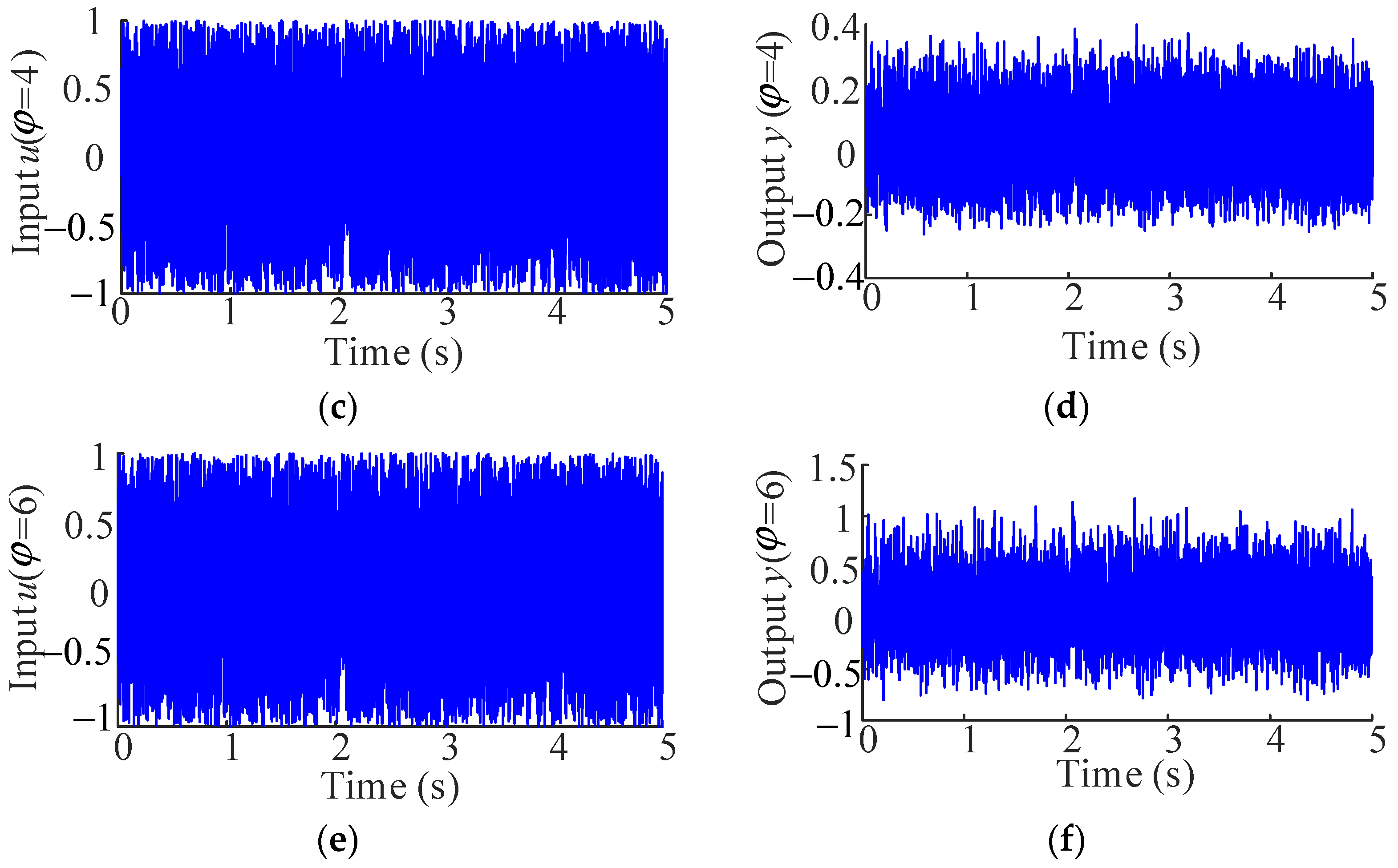
Note that the coefficients of these polynomial functions are randomly generated. Three data sets of 5121 sample points were generated as the input signals, and then the output signals corresponding to the design parameter φ = [2, 4, 6] are obtained by Equations (18) and (19), which are used for modeling. The data sets are shown in Figure 1.


Figure 1.
Input and output signals of φ = [2, 4, 6]. (a) Input signal of φ = 2; (b) output signal of φ = 2; (c) input signal of φ = 4; (d) output signal of φ = 4; (e) input signal of φ = 6; (f) output signal of φ = 6.
In this case, the maximum time lags for both the input and output signals were chosen to be 3, respectively. The degree of the nonlinearity was 3. The results of the identification by using the traditional EFOR algorithm are shown in Table 1. It can be seen in Table 1, the CMS identified by using the traditional EFOR algorithm has all correct terms, and can be written as:
where the coefficient can be expressed as five third-order polynomial functions. The coefficients are obtained by using the LS algorithm, the functions can be written as:

Table 1.
The CMS identified by using the traditional EFOR algorithm.
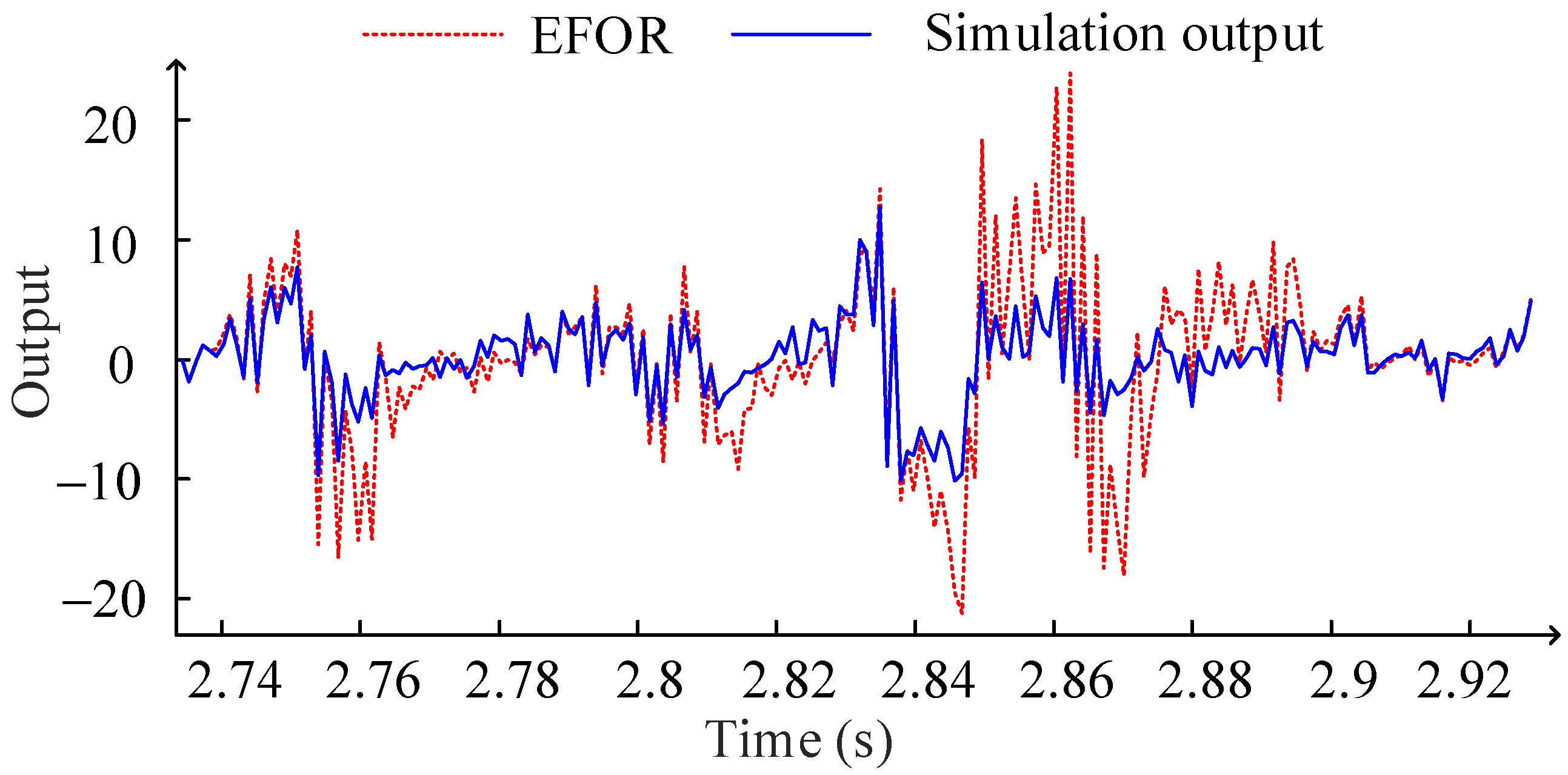
It should be mentioned that the polynomial functions (21) are different with (19) due to the only parts of the data sets are used for modeling. This also shows that the polynomial function obtained by fitting the coefficients of the NARX model and physical parameter values cannot reflect the system characteristics accurately, although the model terms in the CMS are all correct. The EFOR output and simulation result of φ = 10 are compared as shown in Figure 2.
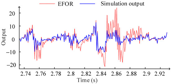
Figure 2.
Comparison between the EFOR output and the simulation output by MPO.
It can be seen in Figure 2, the EFOR output has a significant error for design parameter value not used for the modeling. It also illustrates that the initial NARX-M-for-D cannot reveal the system output accurately by predicting the coefficients through the design parameter value and the predefined functions.
3.2. Evaluation of the Final NARX-M-for-D
In order to facilitate the analysis and design of the nonlinear system by the method of system identification, the WEFOR algorithm is proposed to fix the issue demonstrated in Section 3.1. Firstly, select an arbitrary design parameter value in the interval of interest values to predict the system output, and then compare the results between the predict output and the true value. Secondly, introduce a weight matrix to modify the initial NARX-M-for-D while the error cannot meet the modeling requirement. Finally, derive the weight matrix by using the GA to obtain a more accurate final NARX-M-for-D.
The details of the WEFOR algorithm are summarized as follows:
Step 1: Rewrite Equation (17) into a matrix form as:
where is the coefficient matrix of the NARX models. is the coefficient matrix associated with the design parameters. is the matrix formed by the design parameter as well as the exponents of the design parameter.
Step 2: According to the initial NARX-M-for-D, select a design parameter value which is not used for modeling and then obtain the predicting output by Equations (14) and (17). Introduce the Normalized Mean Square Error (NMSE) [27] to assess the error of the prediction, which can be defined as:
where is the prediction output at time instant t. is the actual output at time instant t. M is the total number of sampling points.
Step 3: Pre-multiplying the right side of Equation (22) by the weight matrix , where is a J × J diagonal matrix, which can be written as:
To find the optimal global value of the weight matrix , in this paper, the GA is applied to minimize the NMSE of all the data sets corresponding to the design parameter (), where is the design parameter value used for the first prediction. The coefficients matrix of the NARX model can then be calculated by:
where is the modified coefficients matrix associated with the design parameters, .
Models (14) and (25) are referred to as the final NARX-M-for-D.
Step 4: Select another design parameter value and then obtain the coefficients of the NARX model by Equation (25). Compare the system output from predicting and simulation, as well as the NMSE calculated by the initial NARX-M-for-D and final NARX-M-for-D to assess the predictive ability of the modified model.
The NMSE of can be derived by:
where is the prediction output at time instant t. is the actual output at time instant t.
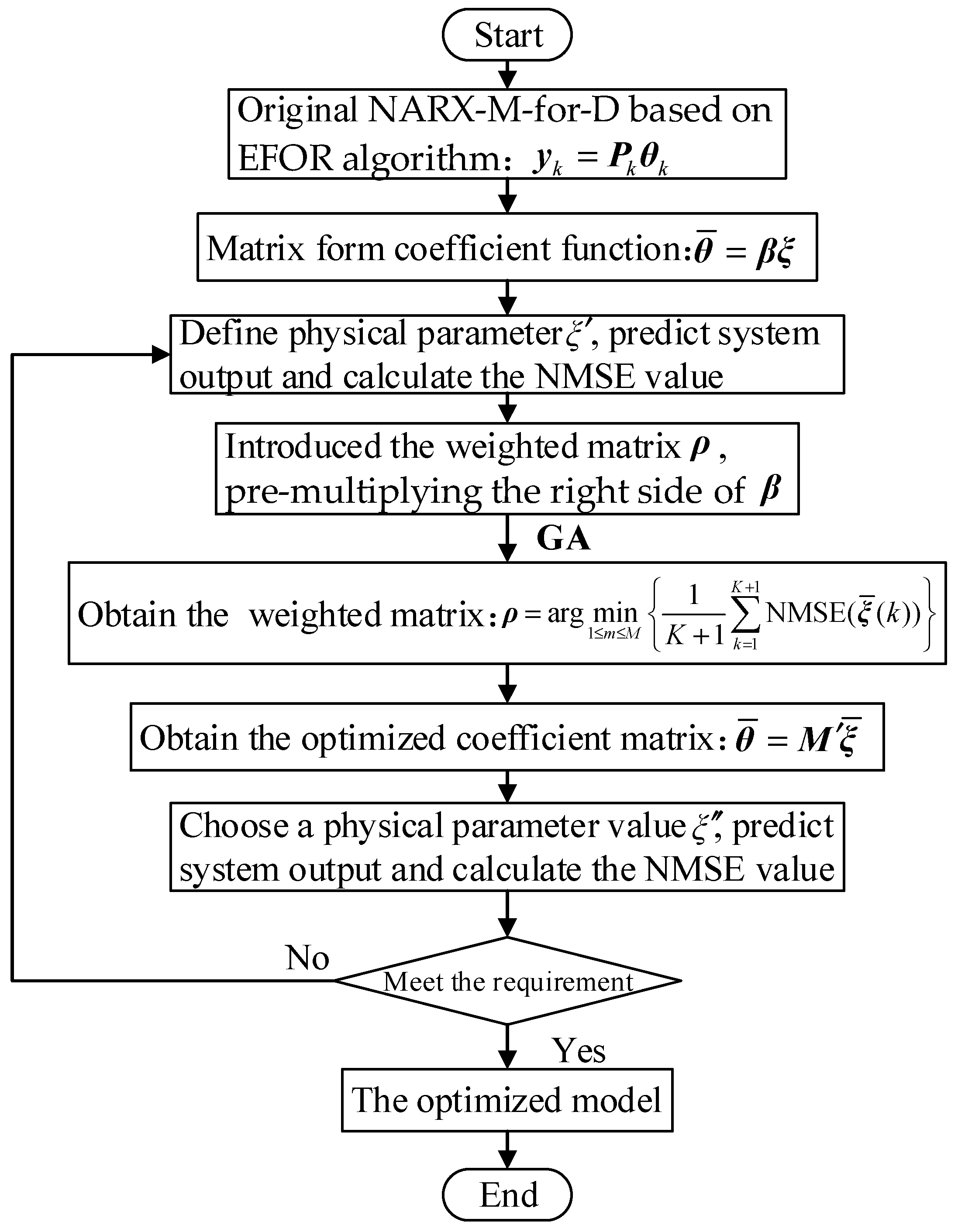
Step 5: If the comparison results in Step 4 cannot meet the requirements, repeat Steps 2 and 3. By repeating, the weight matrix is modified until the output reaches an acceptable level. In the repeating process, the values of design parameter should be chosen in the interval of interest values to modify the relationship function, and then obtain a reliable model. It should be stressed that the parameter and can be selected as any parameter value that close to the parameter values used for initial model identification. The flowchart of Weighted EFOR (WEFOR) algorithm is shown in Figure 3.

Figure 3.
The flowchart of Weighted EFOR (WEFOR) algorithm.
The GA is widely used to obtain the optimum values by minimizing the criterion for the complex optimization problems [28]. It is worth mentioning that the GA has also been widely applied in establishing the NARX models. i.e., Ghosh et al. [29] used the GA to obtain the NARX model with predefined input and output lags and then derived the index of insulin sensitivity. Chen et al. [30] proposed a new fitness function and then identified the number of input–output lags and the coefficients of the NARX model by using the GA. Benabdelwahed et al. [28] proposed a new model structure by expanding the NARX model on Laguerre bases, and the GA was applied to get the optimal Laguerre poles. In these works, the GA was used for model structure detection and parameter estimation.
Compared with these studies, the proposed WEFOR algorithm introduced a weight matrix to modify the relationship between the design parameter and the coefficients of the NARX model by using the GA to minimize the NMSE of all the data sets, this can obtain the optimal global function. The problem that the initial NARX-M-for-D cannot predict the output accurately by an any given design parameter value can be solved by the improved model, which referred to as the final NARX-M-for-D. Therefore, the WEFOR-NARX-M-for-D framework can be applied to reveal the dynamic behaviors of a nonlinear system under certain parameter values better. It should be noted that the proposed WEFOR algorithm introduced a weight matrix to modify the initial identified model, and the values of weight matrix are obtained by GA algorithm, which can be extended to a wide class of nonlinear models. Moreover, comparing with a single LS stage by introducing one more design parameter, the proposed method can obtain a more reliable model because a global optimal model can be obtained by using a genetic algorithm. In addition, the prediction results of the model identified by using the traditional method with more parameters are easier to diverge in some cases.
Remark 2: The function (17) can take any form to connect the design parameter and the coefficients of the NARX model [19], in the absence of prior knowledge, the GA can obtain the global optimum coefficients of the function effectively. Furthermore, it does not matter what type of the actual relationship function is by using the WEFOR algorithm for identification of the NARX-M-for-D.
4. Validation of the WEFOR Algorithm
In order to validate the proposed WEFOR algorithm, the NARX model proposed in Section 3.1 is demonstrated as a numerical study case as well as a cylinder with the bolted joint is illustrated as an experimental case. The predicting results are all obtained by using the MPO method [31], and the calculation of the weight matrix is done by using the GA Toolbox of MATLAB. The results show that the final NARX-M-for-D obtained by using the WEFOR algorithm can predict the output of a nonlinear system accurately in a specific range of parameter values.
4.1. The Numerical Illustrative Example
Consider the NARX model expressed in Equation (18) and the results from Figure 2, the output predicted by the initial NARX-M-for-D have significant errors for the design parameter values not used for the modeling. Therefore, the weight matrix is introduced to modify the initial NARX-M-for-D. In order to obtain the matrix, the GA is used to minimize the NMSE of the data sets of φ = [2, 4, 6, 10]. Figure 4 is the fitness function performance trends in the process of the evolution of the NMSE.
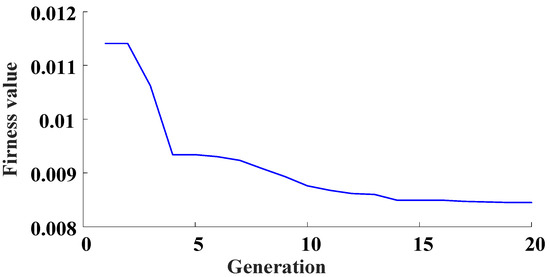
Figure 4.
Evolution of the NMSE in terms of generation.
From Figure 3, the weight matrix can be obtained with twenty generations, which can be written as:
According to Steps 1 and 3 described in Section 3.2, rewrite the polynomial function (21) as a matrix form:
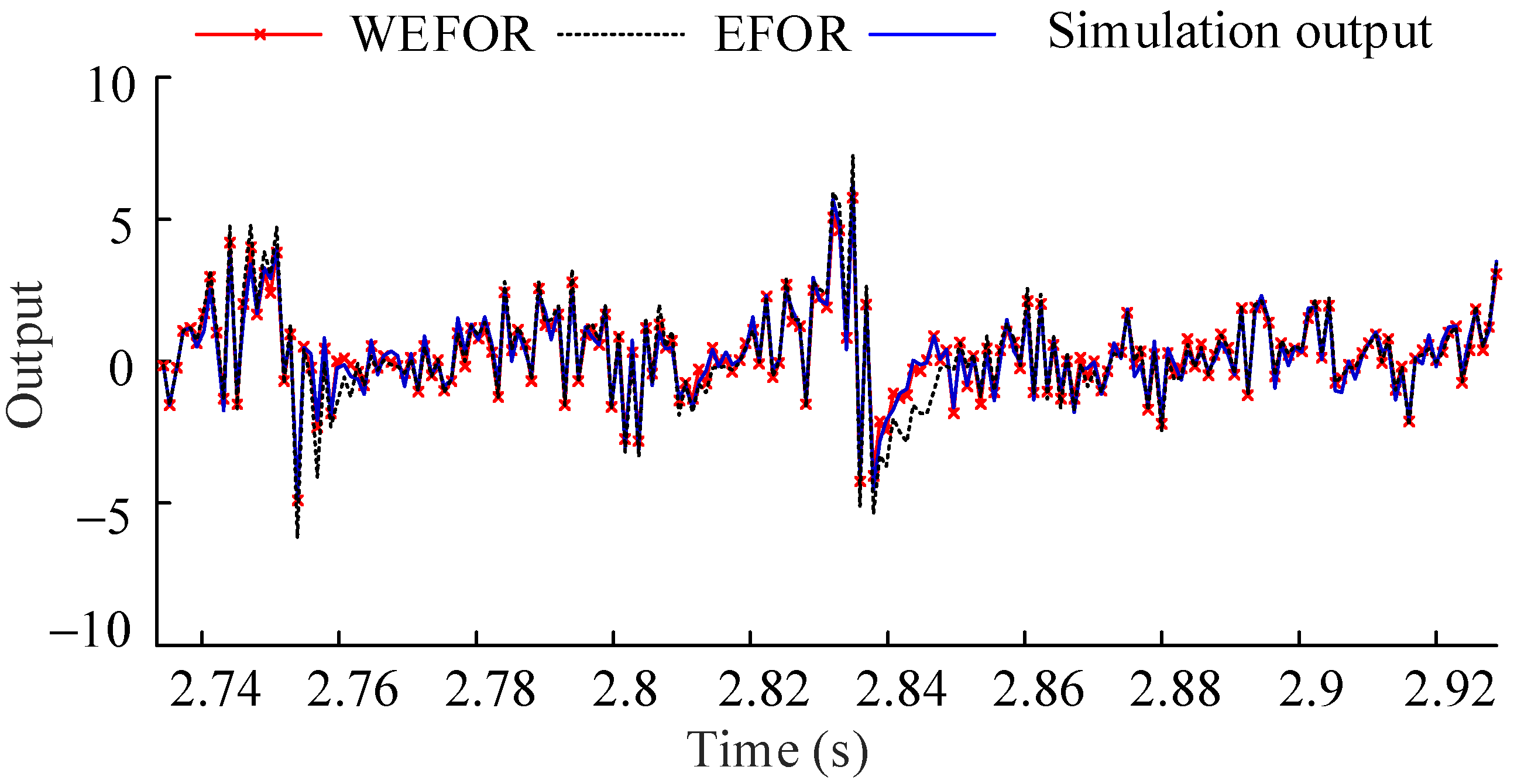
The Models (20) and (28) are the final NARX-M-for-D. And then the data sets of φ = 9 predicted by the final NARX-M-for-D are compared with the EFOR output and the simulation output, as shown in Figure 5.
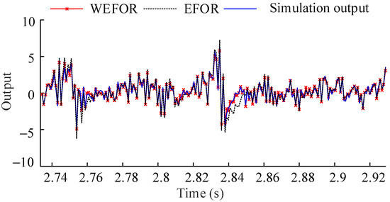
Figure 5.
Comparison among the WEFOR output, the EFOR output, and the simulation output of φ = 9 by MPO.
It can be seen in Figure 5, the WEFOR algorithm has much better predictive ability than the EFOR does. In order to quantitative the predictive ability, the NMSE values calculate from the EFOR output and the WEFOR output was presented in Table 2.

Table 2.
Comparison of the NMSE values.
It can be observed from Figure 2 and Figure 5 and Table 2 that the output predictions of the initial NARX-M-for-D will produce significant errors for the other design parameter values due to the complex relationships between the coefficients of the NARX model and design parameter. It can be seen in Equation (23) that the NMSE value is used to quantify the error between the predicted result and the actual result. Therefore, for the identified model, when the value of NMSE is 0, the obtained model is optimal. However, the error between the predicted result of the identified model and the real result cannot be 0, so the smaller the value is, the more reliable the model is. It should be stressed that the final model was obtained by introducing the corresponding data of another parameter for correction. Therefore, the comparison between EFOR and WEFOR was not made on the same basis of adjustable parameters. The comparison here is to show that the optimized model obtained by WEFOR algorithm has better predictive ability compared with the initial model obtained by EFOR algorithm.
In this numerical illustrative example, the NMSE values provided by the final NARX-M-for-D are less than the initial NARX-M-for-D, it shows that the WEFOR algorithm can obtain the accurate predicting output of the underlying system, and then provide a reliable model for dynamic analysis and design for the nonlinear system. It should be mentioned that the present study is carried out on a workstation (Intel i5-3320M CPU and 16G RAM), the computational time is less than 6 s for the identification of NARX-M-for-D and 2 min for the optimized model in a numerical case study.
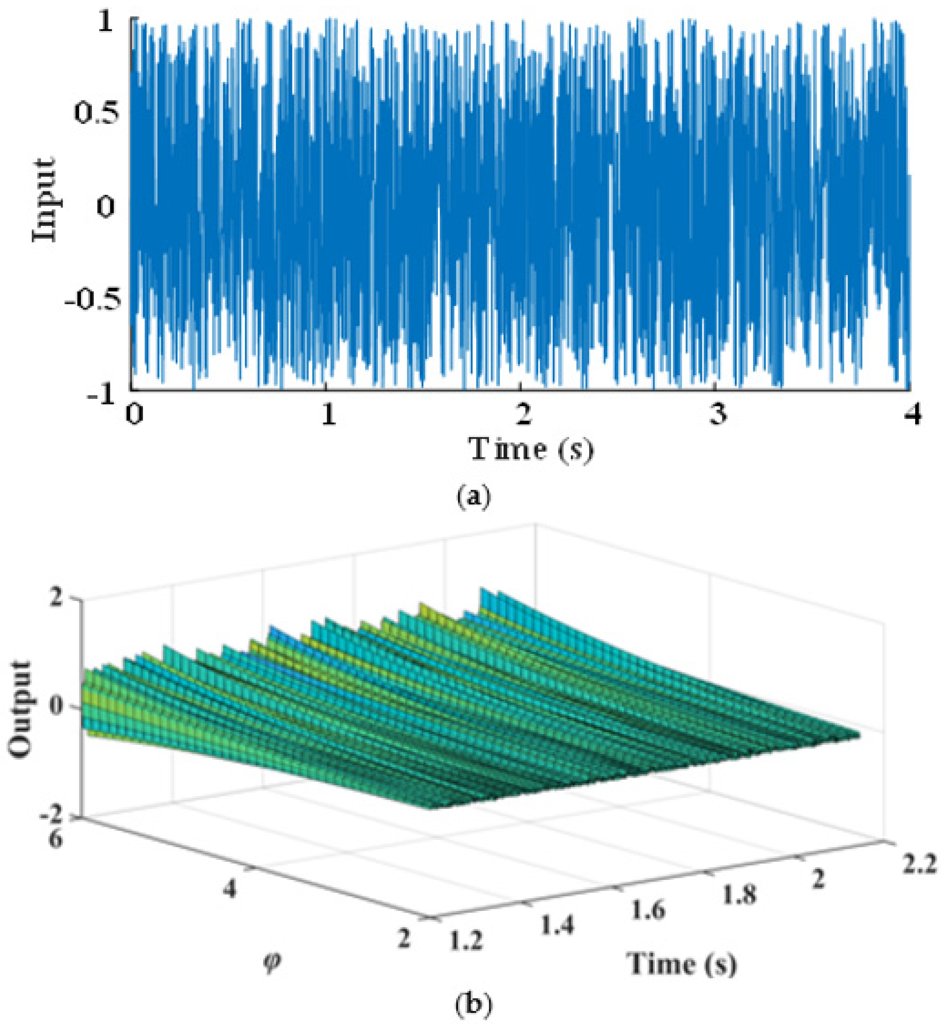
In order to illustrate the process of design by the final NARX-M-for-D, the Gaussian process with zero mean and a variance of is generated as the input signal, as shown in Figure 6a. The predicting outputs corresponding to φ = [2:0.5:6] are obtained by using the MPO method, which is shown in Figure 6b. According to the predicted system output, the corresponding design parameter values can be selected to meet the requirement of design.

Figure 6.
The WEFOR output predict by MPO of φ = [2:0.5:6]. (a) System input and (b) system output.
4.2. Experimental Verification
A cylinder with a bolted joint structure, which belongs to the strong nonlinear class [32] is taken as a test subject for the experimental validation. The acceleration transducer is located at the top of the cylinder wall, the force transducer is connected to the vibration exciter and opposite to the acceleration transducer. The experimental test subject and the test system are shown in Figure 7.
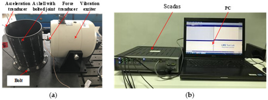
Figure 7.
Experimental test set up. (a) The test subject and (b) the Simcenter Testlab system.
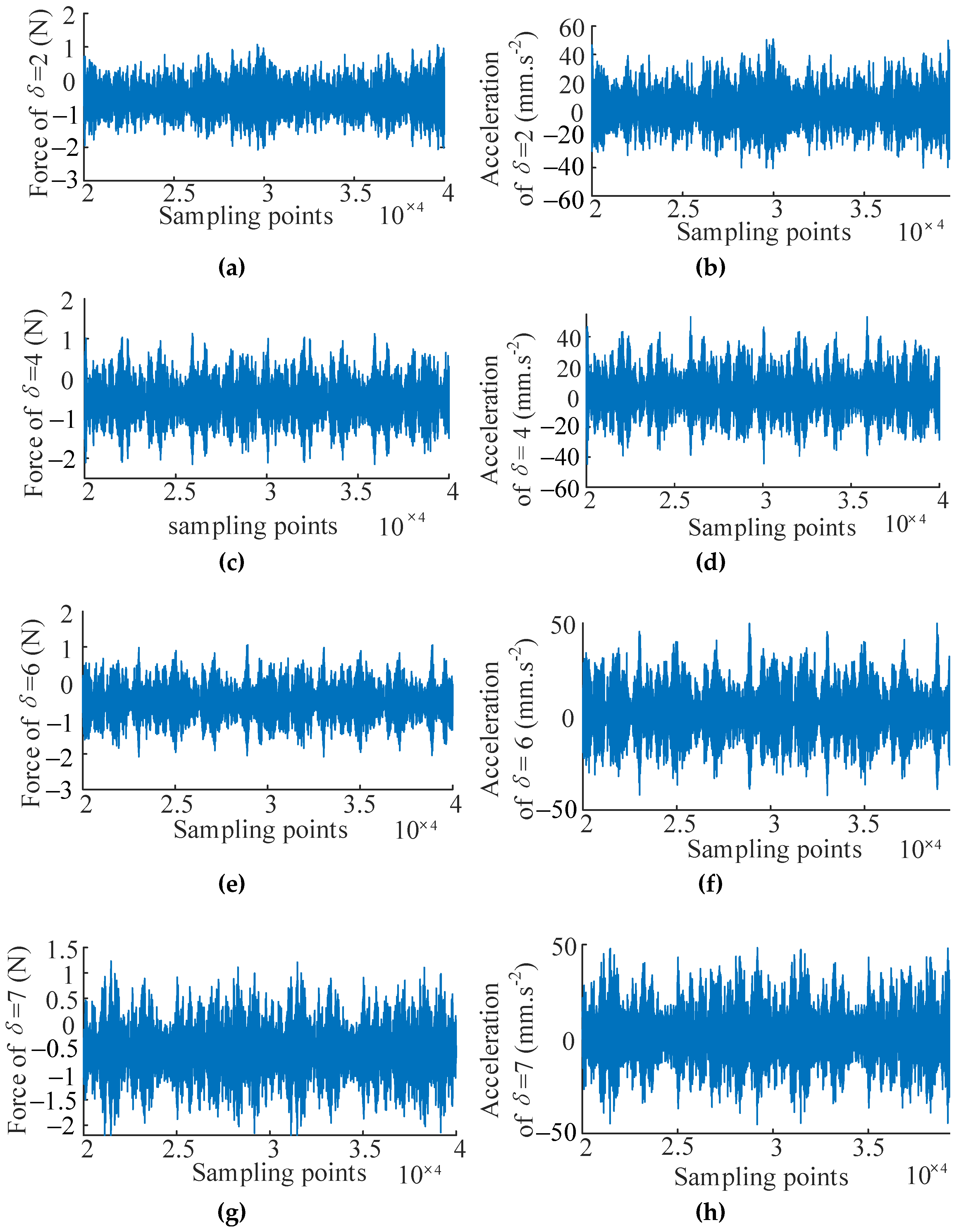
In this case, the Simcenter Testlab system is applied to obtain the input and output signals under different design parameter values of the bolted joint cylinder for verification of the WEFOR algorithm. Denote the input (force) and output (acceleration) variables using u(t) and y(t), respectively. The pre-tightening torque of the bolts is chosen to be the design parameter, which denotes as in this section. Five data sets of 40,000 sample points corresponding to the design parameter δ = [2, 4, 6, 7, 8] Nm were sampled as the input and the output signals. The signals of δ = [2, 4, 6] Nm are used for modeling, and the signals of δ = [7, 8] Nm are used for the modification and validation. The test data sets are shown in Figure 8.
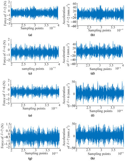

Figure 8.
Input and output signals for modeling and validation. (a) Input signal of δ = 2 Nm; (b) output signal of δ = 2 Nm; (c) Input signal of δ = 4 Nm; (d) output signal of δ = 4 Nm; (e) Input signal of δ = 6 Nm; (f) output signal of δ = 6 Nm; (g) Input signal of δ = 7 Nm; (h) output signal of δ = 7 Nm; (i) Input signal of δ = 8 Nm; and (j) output signal of δ = 8 Nm.
In the experimental case, the maximum time lags for both the input and output signals were chosen to be nu = 3 and ny = 3, respectively. The order of the nonlinearity is selected as l = 3, and the CMS of the bolted joint system identified by using the EFOR algorithm is obtained, the results are shown in Table 3.

Table 3.
The CMS of the bolted joint cylinder.
And then the initial NARX-M-for-D can be obtained as:
where is the coefficient of the initial NARX-M-for-D.
In this case, the coefficients were fitted as third order power-form polynomial functions with respect to the design parameter δ, which can be written as:
The results of were obtained by using the LS algorithm, as shown in Table 4.

Table 4.
Results for the parameters in (30).
The EFOR output of δ = 10 Nm predicted by the Models (29) and (30) are compared with the simulation results, as shown in Figure 9.
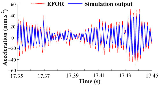
Figure 9.
Comparison between the EFOR output and the simulation output by MPO.
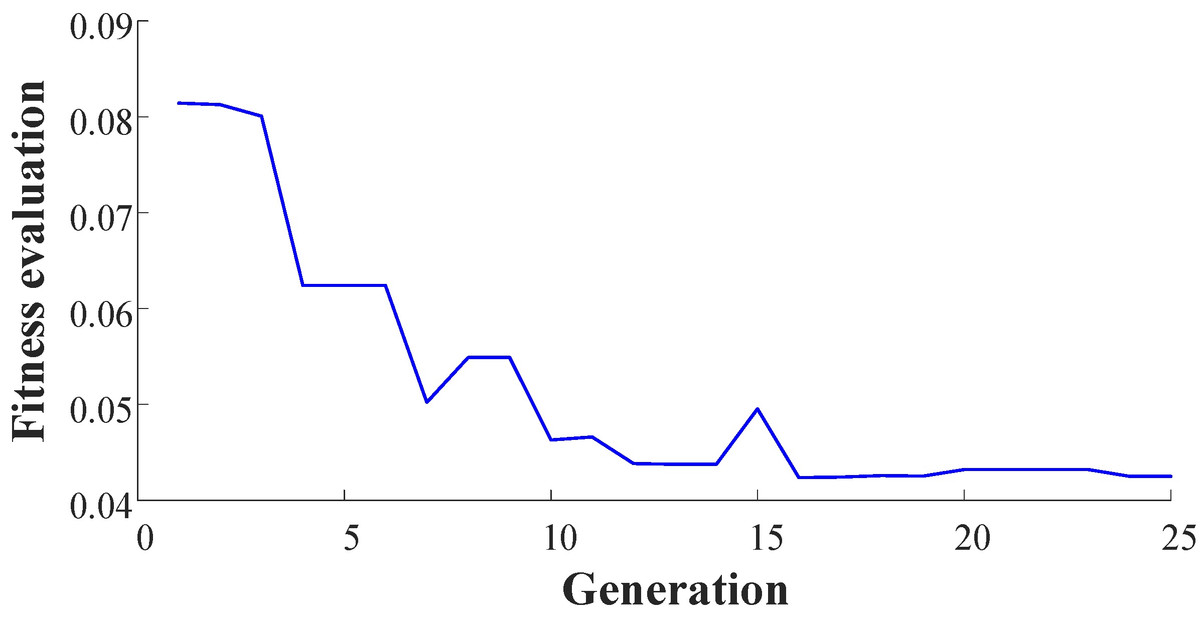
It can be seen in Figure 8, the output predicted by the initial NARX-M-for-D have significant errors. Therefore, the GA is used to minimize the NMSE of the data sets of δ = [2, 4, 6, 8] Nm and obtain the weight matrix. The fitness function performance trends are shown in Figure 10.

Figure 10.
Evolution of the NMSE in terms of generation.
From Figure 9, the values of the weight matrix can be obtained with twenty-five generations, and then the weight matrix is written as:
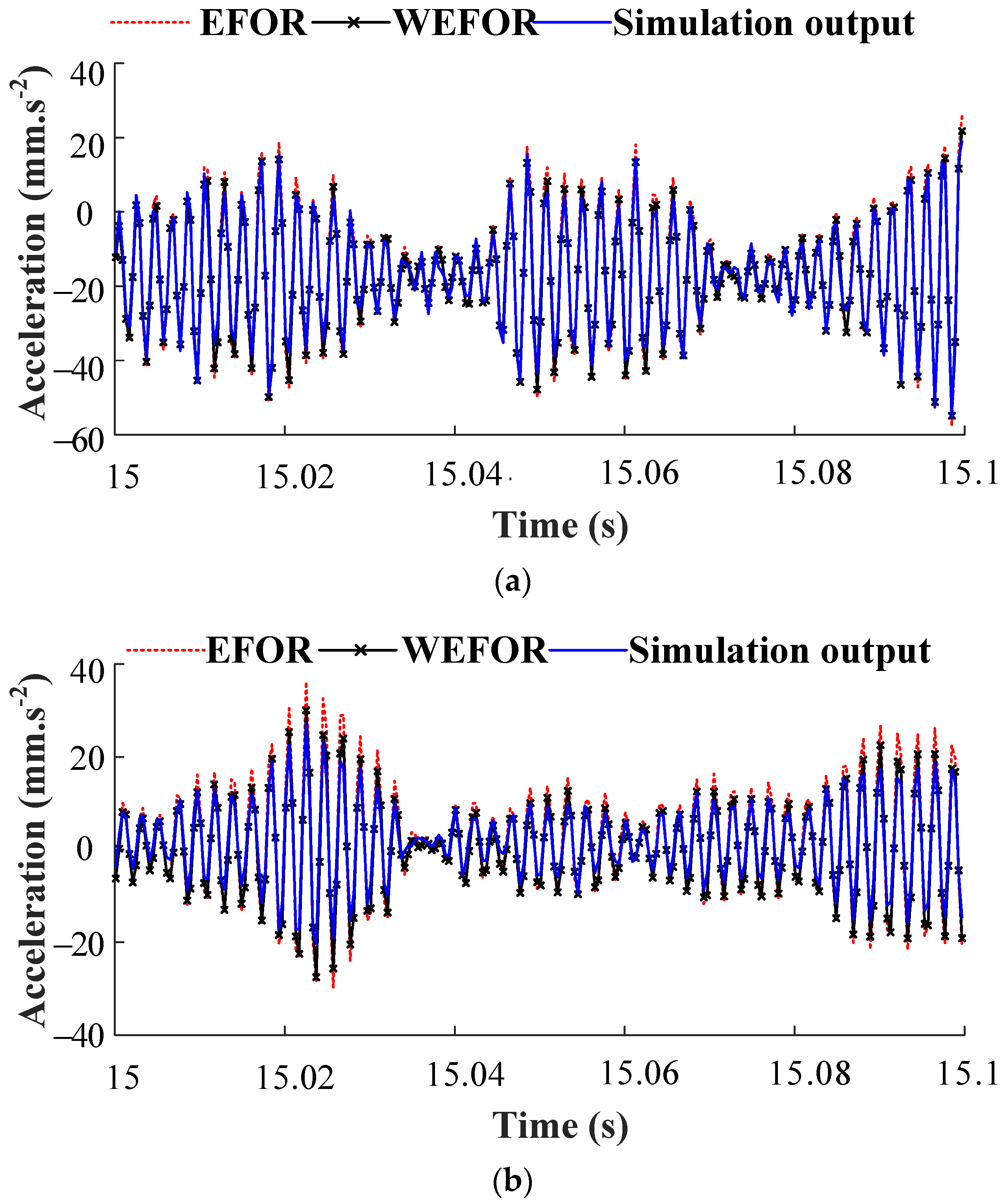
And then the data sets of δ = [7, 8] Nm predicted by the final NARX-M-for-D are compared with the EFOR output and the simulation results, as shown in Figure 11. In order to quantitative the prediction results, the NMSE calculate from the EFOR output, and the WEFOR output was presented in Table 5.
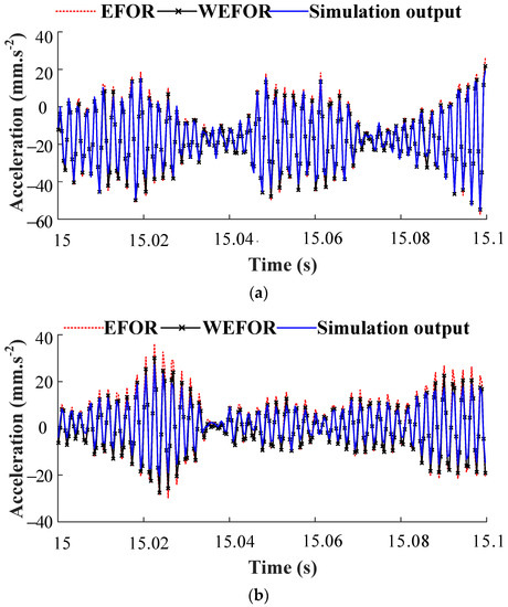
Figure 11.
Comparison among the WEFOR output, the EFOR output, and the simulation output. (a) MPO validation (δ = 7 Nm) and (b) MPO validation (δ = 8 Nm).

Table 5.
Comparison of the NMSE.
It can be observed from Figure 11 and Table 5 that the output predicted by the initial NARX-M-for-D will produce significant errors for the other design parameter in practice. In this experimental study case, the NMSE of the model identified by the WEFOR and EFOR algorithm of δ = 7 Nm are 0.028 and 0.0389, respectively, the NMSE provided by the WEFOR and EFOR algorithm of δ = 8 Nm are 0.0724 and 0.0975, respectively. It shows that the WEFOR algorithm has a better predictive capacity than the EFOR algorithm, and provide a reliable model to predict the output of a nonlinear system under different working conditions accurately. It can be concluded that the WEFOR can predict the system responses under different design parameter values better than the EFOR algorithm. It should be stated that in the experimental case study, the time used for NARX-M-for-D identification is 11 s, and the optimized model is obtained in 3 min.
Take the system input signal measured at δ = 2 Nm as the input for prediction, which is shown in Figure 12a. And then obtain the system output corresponding to δ = [2:0.2:8] Nm through the final NARX-M-for-D by using the MPO method, as illustrated in Figure 11b. The corresponding design parameter values can be chosen to complete the process of system design according to the results in Figure 12b. The results also show that the WEFOR algorithm can obtain a more accurate model to predict the output of the complex nonlinear system, and provide a reliable model for the analysis and design.
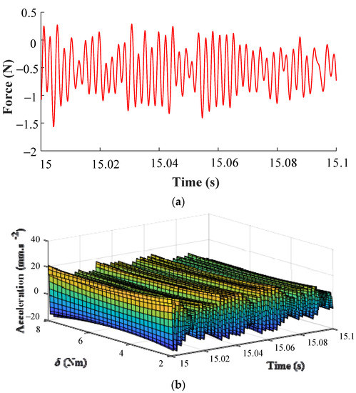
Figure 12.
The WEFOR output obtained by using MPO of δ = [2:0.2:8] Nm. (a) System input and (b) System output.
5. Conclusions
A nonlinear NARX model is demonstrated to show that it is often impossible to obtain the system output by using the traditional EFOR algorithm due to the uncertain and nonlinear relationship between the coefficients of the NARX model and design parameter. To solve this issue, an improved algorithm, referred to as the WEFOR is proposed. The identification process of the WEFOR is conducted by five steps, it can be summarized as follows: (i) establish the initial NARX-M-for-D by using the EFOR algorithm, which defined as the initial NARX-M-for-D; (ii) rewrite the polynomial functions into a matrix form; (iii) select a design parameter value to do the first predict and calculate the NMSE; (iv) introduce a weight matrix, and obtain the values of the matrix by using the GA; and (v) repeat, predict, and calculate the weight matrix until the output meets the requirement.
Both the numerical and experimental studies are conducted to validate the efficiency and accuracy of the new proposed WEFOR algorithm. The results indicate that the output predictions by the traditional EFOR algorithm will produce significant errors for the other design parameter values due to the complex relationships between the coefficients of the NARX models and design parameter. The WEFOR can predict the system responses under different design parameter values better than the EFOR algorithm. The results also show that the WEFOR algorithm can obtain a more accurate model to predict the output of the complex nonlinear system, and provide a reliable model for the analysis and design.
Author Contributions
Y.L.: Conceptualization, methodology, resources, project administration, writing—original draft preparation; D.Y.: software, formal analysis, writing and editing; C.W.: writing—review and editing. All authors have read and agreed to the published version of the manuscript.
Funding
This work was supported by the Science and Technology Project of Liuzhou, China (no. 2019DH10601), National Natural Science Foundation of China (no. 52165055), Science and Technology Project of Guangxi, China (no. GK AD19245149), and Doctoral foundation of Guangxi University of Science and Technology (no. XKB 19Z25).
Institutional Review Board Statement
Not applicable.
Informed Consent Statement
Not applicable.
Data Availability Statement
Data will be made available on reasonable request.
Acknowledgments
Li: Y., Yang, D. and Wen, C. acknowledge the financial support of Guangxi University of Science and Technology, China.
Conflicts of Interest
The authors declare that they have no conflict of interest regarding the publication of this paper.
References
- Qin, Z.Y.; Han, Q.K.; Chu, F.L. Analytical model of bolted disk-drum joints and its application to dynamic analysis of jointed rotor. Proc. Inst. Mech. Eng. Part C J. Mech. Eng. Sci. 2014, 228, 646–663. [Google Scholar] [CrossRef]
- Akinola, T.E.; Oko, E.; Gu, Y.; Wei, H.; Wang, M. Non-linear system identification of solvent-based post-combustion CO2 capture process. Fuel 2019, 239, 1213–1223. [Google Scholar] [CrossRef]
- Sidorov, D.; Muftahov, I.; Tomin, N.; Karamov, D.; Panasetsky, D.; Dreglea, A.; Foley, A.A. Dynamic Analysis of Energy Storage With Renewable and Diesel Generation Using Volterra Equations. IEEE Trans. Ind. Inform. 2020, 16, 3451–3459. [Google Scholar] [CrossRef] [Green Version]
- Zhu, Y.; Lang, Z.Q. A new convergence analysis for the Volterra series representation of nonlinear systems. Automatica 2020, 111, 108599. [Google Scholar] [CrossRef]
- Csurcsia, P.Z.; Peeters, B.; Schoukens, J. User-friendly nonlinear nonparametric estimation framework for vibro-acoustic industrial measurements with multiple inputs. Mech. Syst. Signal Pract. 2020, 145, 106926. [Google Scholar] [CrossRef]
- Birpoutsoukis, G.; Csurcsia, P.Z.; Schoukens, J. Efficient multidimensional regularization for Volterra series estimation. Mech. Syst. Signal Pract. 2018, 104, 896–914. [Google Scholar] [CrossRef] [Green Version]
- Haryanto, A.; Hong, K.S. Maximum likelihood identification of Wiener-Hammerstein models. Mech. Syst. Signal Pract. 2013, 41, 54–70. [Google Scholar] [CrossRef]
- Liu, Y.; Bai, E. Iterative identification of Hammerstein systems. Automatica 2007, 43, 346–354. [Google Scholar] [CrossRef]
- Wills, A.; Schon, T.B.; Ljung, L.; Ninness, B. Identification of Hammerstein-Wiener models. Automatica 2013, 49, 70–81. [Google Scholar] [CrossRef] [Green Version]
- Leontaritis, I.J.; Billings, S.A. Input-output parametric models for non-linear systems Part I: Deterministic non-linear systems. Int. J. Control 1985, 41, 26. [Google Scholar] [CrossRef]
- Leontaritis, I.J.; Billings, S.A. Input-output parametric models for non-linear systems Part II: Stochastic non-linear systems. Int. J. Control 1985, 41, 329–344. [Google Scholar] [CrossRef]
- Ayala Solares, J.R.; Wei, H. Nonlinear model structure detection and parameter estimation using a novel bagging method based on distance correlation metric. Nonlinear Dynam. 2015, 82, 201–215. [Google Scholar] [CrossRef]
- Rashid, M.T.; Frasca, M.; Ali, A.A.; Ali, R.S.; Fortuna, L.; Xibilia, M.G. Nonlinear model identification for Artemia population motion. Nonlinear Dynam. 2012, 69, 2237–2243. [Google Scholar] [CrossRef]
- Ge, X.B.; Luo, Z.; Ma, Y.; Liu, H.P.; Zhu, Y.P. A novel data-driven model based parameter estimation of nonlinear systems. J. Sound Vib. 2019, 453, 188–200. [Google Scholar] [CrossRef]
- Bayma, R.S.; Zhu, Y.P.; Lang, Z.Q. The analysis of nonlinear systems in the frequency domain using Nonlinear Output Frequency Response Functions. Automatica 2018, 94, 452–457. [Google Scholar] [CrossRef]
- Billings, S.A. Nonlinear System Identification: NARMAX Methods Nonlinear System Identification: NARMAX Methods in the Time, Frequency, and Spatio-Temporal Domains; John Wiley & Sons: Chichester, UK, 2013. [Google Scholar]
- Wei, H.L.; Lang, Z.Q.; Billings, S.A. Constructing an overall dynamical model for a system with changing design parameter properties. Int. J. Model. Identif. Control 2008, 5, 93–104. [Google Scholar] [CrossRef]
- Zhu, Y.; Lang, Z.Q. Design of Nonlinear Systems in the Frequency Domain: An Output Frequency Response Function-Based Approach. IEEE Trans. Contr. Syst. Technol. 2017, 99, 1–14. [Google Scholar] [CrossRef] [Green Version]
- Liu, H.; Zhu, Y.; Luo, Z.; Wang, F. Identification of the dynamic parametrical model with an iterative orthogonal forward regression algorithm. Appl. Math. Model. 2018, 64, 643–653. [Google Scholar] [CrossRef]
- Piroddi, L.; Spinelli, W. An identification algorithm for polynomial NARX models based on simulation error minimization. Int. J. Control 2003, 76, 1767–1781. [Google Scholar] [CrossRef]
- Billings, S.A.; Wei, H. Sparse Model Identification Using a Forward Orthogonal Regression Algorithm Aided by Mutual Information. IEEE Trans. Neural Netw. 2007, 18, 306–310. [Google Scholar] [CrossRef] [PubMed]
- Guo, Y.; Guo, L.Z.; Billings, S.A.; Wei, H. An iterative orthogonal forward regression algorithm. Int. J. Syst. Sci. 2015, 46, 776–789. [Google Scholar] [CrossRef]
- Liu, Y.; Li, J.; Wang, T.; Ding, Y.; Wang, G. Study on the friction resistance calculation method of a flexible shaft of wire rope based on genetic algorithm. Mech. Adv. Mater. Struc. 2021, 1–15. [Google Scholar]
- Wei, H.L.; Zheng, Y.; Pan, Y.; Coca, D.; Li, L.M.; Mayhew, J.E.; Billings, S.A. Model estimation of cerebral hemodynamics between blood flow and volume changes: A data-based modeling approach. IEEE Trans. Biomed. Eng. 2009, 56, 1606–1616. [Google Scholar]
- Liu, H.; Zhu, Y.; Luo, Z.; Han, Q. PRESS-based EFOR algorithm for the dynamic parametrical modeling of nonlinear MDOF systems. Front. Mech. Eng. 2018, 13, 390–400. [Google Scholar] [CrossRef]
- Wolberg, J. Data Analysis Using the Least-Squares Method; Springer: Berlin/Heidelberg, Germany, 2006. [Google Scholar]
- Favier, G.; Kibangou, A.Y.; Bouilloc, T. Nonlinear system modeling and identification using Volterra-PARAFAC models. Int. J. Adapt. Control 2012, 26, 30–53. [Google Scholar] [CrossRef] [Green Version]
- Benabdelwahed, I.; Mbarek, A.; Bouzrara, K.; Garna, T. Non-linear system modelling based on NARX model expansion on Laguerre orthonormal bases. IET Signal Process 2018, 12, 228–241. [Google Scholar] [CrossRef]
- Ghosh, S.; Maka, S. Genetic algorithm based NARX model identification for evaluation of insulin sensitivity. Appl. Soft Comput. 2011, 11, 221–226. [Google Scholar] [CrossRef]
- Chen, Q.; Worden, K.; Peng, P.; Leung, A.Y.T. Genetic algorithm with an improved fitness function for (N)ARX modelling. Mech. Syst. Signal Pract. 2007, 21, 994–1007. [Google Scholar] [CrossRef]
- Ma, Y.; Liu, H.; Zhu, Y.; Fei, W.; Zhong, L. The NARX Model-Based System Identification on Nonlinear, Rotor-Bearing Systems. Appl. Sci. 2017, 7, 911. [Google Scholar] [CrossRef]
- Brake, M.R.W. The Mechanics of Jointed Structures; Springer: Berlin/Heidelberg, Germany, 2018. [Google Scholar]
Publisher’s Note: MDPI stays neutral with regard to jurisdictional claims in published maps and institutional affiliations. |
© 2021 by the authors. Licensee MDPI, Basel, Switzerland. This article is an open access article distributed under the terms and conditions of the Creative Commons Attribution (CC BY) license (https://creativecommons.org/licenses/by/4.0/).


