Research on Collaborative Efficiency Evaluation of Complex Supplier Network under the Background of Intelligent Manufacturing

Abstract

Supplier network collaborative efficiency evaluation is important content in the transformation and upgrading of intelligent manufacturing enterprises. Aiming at the shortcomings of existing methods, this paper proposes a new method to evaluate the collaborative efficiency of internal members of a complex supplier network based on complex network theory. Based on the analysis of the characteristics of the complex supplier network, from the perspective of the system, the macro supplier network is divided into multiple multi-level supplier micro subsystems with manufacturing enterprises as the core. In order to reasonably quantify the collaboration relationship of members in the subsystem structure model, the collaboration entropy is introduced as a measurement tool, and combined with the hesitation fuzzy scoring function, and the collaborative evaluation model of the complex supplier network is constructed. By quantifying the collaboration relationship among the members in the subsystem and summarizing it step by step and iteratively, the collaborative efficiency evaluation of the complex supplier network from local to overall is realized. Finally, taking a large battery manufacturing enterprise in China as an example, the proposed method is used to calculate the collaboration entropy, collaborative efficiency, and collaboration ratio of members at different supplier network levels. The results verify the effectiveness of the model.

1. Introduction

With the continuous deepening of a new round of scientific and technological revolution and industrial reform, the integrated development of digitization, networking, and intelligence in the manufacturing industry is constantly breaking through new technologies and giving birth to new business forms. Intelligent manufacturing has become an important starting point to promote the transformation and upgrading of the manufacturing industry and accelerate the high-quality development of the manufacturing industry [1]. In order to promote China’s transformation from a manufacturing power to a manufacturing power, the State Council of China has issued the “made in China 2025” plan, which aims to optimize the economic structure, improve international competitiveness, and smoothly connect with German industry 4.0, which has attracted the attention and attention of many scholars [2,3].

In the context of intelligent manufacturing, manufacturing enterprises regard suppliers as an extension of their production system [4], and the relationship between manufacturing enterprises and suppliers has gradually shifted from the traditional “capital material” supply-demand bilateral transaction to the strategic partnership alliance of “main manufacturer supplier” mode [5,6,7]. With the change of identity, some suppliers in the supply chain not only undertake the supply function of materials, but also integrate into the product R&D and manufacturing links as an important partner of the main manufacturer, so as to share the risks and corresponding benefits for the main manufacturer. The main manufacturer also obtains the innovation resource elements attached to the supplier in the continuous and dynamic business communication with the supplier, so as to promote the improvement of the enterprise’s product competitiveness and the realization of the strategic goal [8,9,10]. The supplier network is a supply system based on close cooperation with multiple suppliers around core manufacturing enterprises [8]. As the core of the organization, how to make more efficient and sustainable use of suppliers’ resources and capabilities is both an opportunity and a challenge for the main manufacturers.

At present, the research on the supplier network at home and abroad is still in a discrete state. The results focus on the interpretation of the network structure, network membership, and its behavior, as well as the abstract overview of control strategies, but they generally ignore the role of synergy, a key element. This has failed to put forward practical solutions to the low efficiency of supplier network collaboration in combination with the actual needs of enterprises in the process of moving forward to intelligent manufacturing. The research conclusions provide relatively broad guidance for practice. Supplier network collaboration is a series of collaborative activities centered on product manufacturing based on the supply business collaboration platform jointly set up by core enterprises and their suppliers. The purpose is to improve the operation efficiency of enterprises and suppliers through the high cooperation between supply and production. Efficient collaboration means the whole process optimization from product R&D to production, from supply chain support to after-sales service, which is exactly one of the important conditions for the transformation and upgrading of the manufacturing industry to the intelligent manufacturing field.

When a new round of global industrial revolution with intelligent manufacturing as the core comes, most enterprises in reality do not transform their competitive advantages through supplier network collaboration as described in relevant theories but face a series of reform difficulties and pain points. There are many reasons for this situation. It comes from the competitive relationship within the supplier network. There are differences among node enterprises in the operation mode, business strategy, and interest demand, resulting in a lack of goal consistency among supplier network members. This lack directly or indirectly affects the value release and value creation of node enterprises in the network. In addition, the opacity and asymmetry of information often lead to opportunistic risk [8,10], making it difficult for the synergy between the winner manufacturer and the supplier to develop in the expected direction. Therefore, using appropriate scientific methods to describe and quantify the network synergy and collaboration efficiency, accurately evaluate the progress and effect of the transformation and upgrading of the main manufacturer, and encourage the members of the supplier network to form close synergy is an important scientific problem that the main manufacturer urgently needs to solve in the supplier network management, and it is also an important content of this paper.

In recent years, the application of complex network theory to study the supply chain network has attracted extensive attention in academic circles [11]. Chen and Zhang [12] believe that the supply chain system is a complex self-organizing and adaptive network system, and the perspective of the complex network is conducive to reveal the characteristics of this kind of system. Fan and Liu [13] took the characteristics of supply network complexity and found that the application of complex network theory is helpful for enterprises to better evaluate the supply chain structure, coordinate the behavior of member enterprises, and improve the stability of supply chain. With the deepening of research, some scholars try to improve and innovate on the basis of the existing models, pointing out that the connection number and connection rate of nodes in the supply chain network are not only related to the time factor [14], but also affected by the attraction between nodes, location parameter, edge benefit, and supply chain life cycle. Based on this, a complex supply chain network evolution model based on factor X is proposed. The above scholars have studied the supply chain network from different angles, which shows that the supply chain network has separated from the category of simple topology and has the characteristics of a complex network.

The concept of a complex supplier network (CSN) is based on the simplification of the complex supply chain network. As we all know, a supply chain with a complete structure and function is generally composed of five parts: the main manufacturer, supplier, distributor, retailer, and final consumer group. The increment of the product value depends on the multi-level transmission of the supply chain, which involves multiple manufacturing and supply links. Compared with retailers and distributors who only occupy a small share at the end of the supply chain, suppliers and manufacturers in the supply chain have absolute quantitative advantages. Therefore, reducing a certain number of distribution module nodes for a complex supply chain network will not affect the overall shape and function of the network. By eliminating distributors, retailers, and customers, this paper will be carried out under the framework of CSN.

Due to the complex form and large number of nodes of the complex supplier network, in order to achieve the purpose of indifferently depicting the collaboration relationship of members, this paper chooses to cut and divide the complex supplier network into multiple multi-level micro subnetworks with manufacturing enterprises as the core. For subnetworks, the collaboration entropy function, which is mostly used to quantify the enterprise management business collaboration relationship [15,16], is creatively popularized in the field of complex supplier networks, and a collaborative efficiency evaluation model of complex supplier networks is constructed to quantify the collaborative interaction behavior among network members, so as to evaluate the collaborative efficiency of complex supplier networks. In addition, in order to reasonably and dynamically determine the collaboration critical value used to divide the collaboration state, an improved hesitation fuzzy scoring function based on collaboration preference is introduced to avoid the impact of decision-makers’ absolute and subjective judgment on the research [17].

2. Materials and Methods

2.1. Complex Supplier Network

The academic definition of complex networks is networks with some or all of the properties of self-organization [18], self-similarity [19], attractor [20], small world [21], and scale-free [14]. More and more realistic studies show that the network abstracted from practical problems in the real world is neither a regular network nor a random network but a complex network, such as a computer network [22], social interpersonal network [23], financial system network [24], epidemic transmission network [25], etc. Because the form of the supply chain has an important impact on its own performance, the early chain supply chain and the supply chain network formed by its expansion have been difficult to describe and explain the complex interaction between enterprises. In order to meet the needs of the current changeable market environment and future development trend, the traditional supply chain network has gradually changed from a simple network topology to a complex network [26]. CSN is a supply system with complex network characteristics based on the close cooperation with multiple suppliers around the main manufacturer.

2.2. Characteristic Analysis of CSN

The external and endogenous characteristics of CSN are as follows.

1. Scale free. Affected by the evolution mode of the preferred connection of network nodes, CSN has a Matthew effect in its structure and a power-law distribution in the degree distribution. The power index is usually in the range of two to three. This kind of complex network with a power-law distribution is called a scale-free network. In scale-free networks, nodes are heterogeneous, and the connections between nodes do not obey a uniform distribution. Most nodes are connected with only a few nodes, and the degree value is very low. However, there are a few hub nodes that play a key role in the operation and maintenance of the overall network. This type of node is associated with many nodes in the network, and the degree value is very high. From the perspective of network evolution, with the continuous participation of member enterprises, the network scale expands. The identity of large enterprises and their potential resources means that new member enterprises prefer to establish cooperative relations with them. A small number of large enterprises with a large number of partners, and a large number of minor enterprises with only a small number of partners have gradually emerged in the network. Around the main manufacturer, a product value chain from product raw material supply, production, processing, sales, and transportation has been formed [27,28,29], which fully reflects the scale-free nature.

2. Adaptability. Adaptation is an interactive process of the relationship, which is reflected in the construction and cooperation of the complex supplier network. The mutual selection and mutual trust of the internal members of the supplier network with the main manufacturer as the core is the basis for generating value-added collaborative benefits. For the raw material procurement and supply links in the product manufacturing process, the main manufacturer actively and spontaneously takes incentive measures for the members of the subordinate supplier network to coordinate and control the development of the supplier network.

3. Embedded evolution. In the supplier network with good economic benefits, the main manufacturer and the members of the supplier network establish a partnership and form a continuous embedded connection. A good embedded relationship can enhance the sense of integrity and trust among network members, so as to contribute to the small-scale sharing of information and timely feedback of problems, and finally achieve a high degree of coordination between material supply and production. At the same time, the embedded evolution of the supplier network is conducive to improving the competitiveness of enterprises. This implicit benefit is often easy to be ignored. In fact, this relative index is an important way for enterprises to calmly and quickly respond to market changes and seize market opportunities. Excellent enterprise competitiveness brings a virtuous circle for continuous collaborative cooperation.

2.3. Entropy Theory

Since the dissipative structure theory and synergy theory were put forward in the 1970s, nonlinear science has experienced a long history of development. A series of system complexity problems represented by uncertainty measurement, information entropy, management entropy, and collaborative evolution have always been the research hotspot. Entropy theory has become one of the important theories of complex science.

With regard to the application of entropy theory in collaborative evaluation, the Chinese scholars Song et al. [30] have proposed collaborative parameters, such as collaborative span, collaborative trajectory, collaborative mechanism, and collaborative efficiency, around the enterprise organization system; established an index evaluation system with organizational synergy as the core; and built a mathematical model of collaborative entropy evaluation from the multi-dimensional aspects of collaborative structure, collaborative mode, and collaborative function. The research conclusion is of great significance for the expansion of collaborative management. This paper is the re-extension of entropy theory on the basis of this research. Entropy, as a tool to describe the degree of order, can reflect the order of the supplier network by measuring the degree of chaos in the supplier network. Therefore, it has good adaptability in solving the problem of supplier network collaborative management.

2.3.1. Information Entropy

In 1948, Shannon, the father of information theory, put forward the concept of information entropy with the help of thermodynamic knowledge. Information entropy [31] is a measurement tool to describe the uncertainty of information sources according to the contribution of things to information. Within the system $S$, $P_i$ is the probability of a discrete event, and the information entropy of the discrete events can be expressed as:

$$H\left(S\right)=-{\displaystyle \sum P_i}\log P_i,i=1,2,\dots ,k$$

(1)

Extended to the supplier network, $f_i$ is the chain number of collaboration relationships of the supplier, and $f$ is the sum of $f_i$. The corresponding collaboration entropy of suppliers can be expressed as:

$$H\left(S\right)=-{\displaystyle \sum \frac{f_i}{f}}\log \frac{f_i}{f}, f={\displaystyle \sum f_i}, i=1,2,\dots ,k$$

(2)

2.3.2. Entropy Weight Method

Information entropy is applied to the collaborative efficiency evaluation. For an index, the smaller the information entropy, the greater the variation degree of the index. Specifically, the more information that can be provided, the greater the contribution to the system [32]. This feature of information entropy is used to solve the index weight portion of multi-attribute decision-making problems [33].

Take a multi-attribute decision-making problem as an example. There are $r$ evaluation objects and $m$ evaluation indexes. For the original data matrix $A$, $A={\left(a_{ij}\right)}_{r\times m}$, $a_{ij}$ denotes the evaluation value of the j-th index of the i-th evaluation object.

Step 1: To solve the problem of inconsistent measurement units for each indicator, the original data matrix $A$ is homogenized to obtain the data matrix $B$:

$$B={\left(b_{ij}\right)}_{r\times m}, i\in r, j\in m$$

Step 2: The columns of data matrix $B$ are normalized to obtain the index evaluation matrix $C$:

$$C={\left(c_{ij}\right)}_{r\times m}, c_{ij}=\frac{b_{ij}}{{\displaystyle {\sum }_{i=1}^r{b}_{ij}}}, {\displaystyle \sum c_{ij}}=1, i\in r, j\in m$$

Step 3: The output entropy of the j-th evaluation index is calculated:

$e_j=-\frac{1}{\ln r}{\displaystyle \sum _{i=1}^r{c}_{ij}}\ln c_{ij}$, $0\le e_j\le 1$. (Note: if $c_{ij}=0$, then $c_{ij}\ln c_{ij}=0$)

Step 4: The weight coefficient of each evaluation index is calculated:

$$w_i=\frac{1-e_j}{m-{\displaystyle \sum _{v=1}^m{e}_v}}$$

3. CSN Collaborative Efficiency Evaluation Model

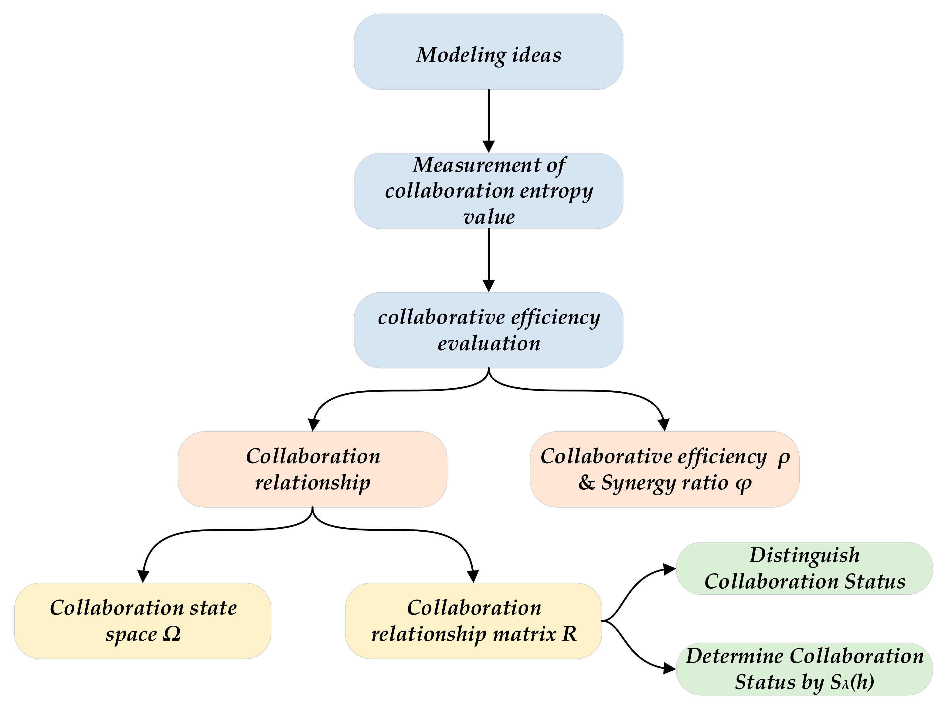
3.1. Chapter Overview

Due to the numerous concepts, definitions, and formulas involved in this chapter, in order not to omit relevant contents and better convey the model construction process, the proposed method flow is shown in Figure 1.

3.2. Modeling Ideas

The development of economic globalization makes the cooperation between enterprises increasingly closer, and virtually deepens the role overlap and relationship complexity between enterprises. The same enterprise plays different roles in the supply chain. For example, the manufacturing enterprise is not only responsible for production, but also undertakes the supply function of suppliers.

In order to overcome the impact of repeated calculation caused by role aliasing between main manufacturers and suppliers, this paper takes the structural characteristics of the complex supplier network as the starting point. According to the scale-free structural characteristics mentioned above, the macro complex supplier network is cut and divided into multiple micro sub networks with the main manufacturer in the local network as the vertex. As shown in Figure 2, by splitting the complex supplier network, the structural transformation of complex three-dimensional cyberspace from complexity to simplicity is realized. The system is an organic whole with specific functions composed of interactive and interdependent parts. Therefore, the complex supplier network can be mapped into a system, and the micro subnetwork generated by cutting is a subsystem, forming a parent subsystem relationship with the complex supplier network.

The nodes in the subsystem are treated in the same direction. The sub nodes, which are scattered around the hub node, are rotated and pulled to the lower part of the hub node, so that the nodes belonging to different supply levels are relatively unified in the structural model. On this basis, in order to further simplify the structural model, the isotropic sub nodes are placed in the same plane as the hub nodes to realize the transition of the structural model from three-dimensional to two-dimensional. As shown in Figure 3, the subsystem has the characteristics of self-similarity in structure, which shows that the local shape is similar to the overall shape, and there are similar parts in the local, which are constantly repeated and nested layer by layer to form a fractal diagram.

According to the above model structure simplification steps, a planar multi-level supplier network with manufacturing enterprise as the core and hierarchical division is obtained. Studies have shown that other enterprises that have business dealings with the supplier in the expanded supply network may affect the efficiency of the supplier [34]. Therefore, from the perspective of the main manufacturer, it is necessary to understand the collaboration status of the extended secondary and even tertiary suppliers. Considering that there are many levels in a complete supplier network, and the coordination measurement methods among suppliers at all levels are similar, due to space constraints, only the first three supply levels starting from the top root node of the subsystem are intercepted for a specific coordination entropy solution and coordination efficiency evaluation. As shown in Figure 4, the nodes are arranged in order from upstream to downstream: root node manufacturer (RM), branch node supplier (BS), and leaf node supplier (LS). They refer to the main manufacturer, primary supplier, and secondary supplier in order.

The subsystem structure model is defined as the Root-Branch-Leaf model (RBL model), and the number of suppliers in the BS layer is set as $\pi$ and the number of suppliers in the LS layer as $\epsilon$. $S_{\mu }$ is the $\mu$-th supplier for the BS layer. The supplier unit composed of BS layer suppliers is marked as $U_0$, where $U_0=\left\{S_1,\dots ,S_{\mu },\dots ,S_{\pi }\right\}$. $S_{\mu \omega }$ is the subordinate supplier of $S_{\mu }$, and the supplier unit formed by $S_{\mu \omega }$ is recorded as $U_{\mu }$, where $U_{\mu }=\left\{S_{\mu 1},\dots ,S_{\mu \omega },\dots ,S_{\mu \theta }\right\}$, $U_k=\left\{U_0,U_{\mu }\right\}$, ${\displaystyle \sum _{\mu =1}^{\pi }{\displaystyle \sum _{\omega =1}^{\theta }{S}_{\mu \omega }}}=\epsilon$.

3.3. Measurement of the Collaboration Entropy Value

In order to reasonably quantify the collaboration relationship of members in the subsystem structure model, the collaboration entropy function is introduced as a measurement tool. CSN is formed in the two-way selection process between main manufacturers and suppliers. This dynamic process is always accompanied by the replacement behavior of new members joining and old members quitting with the medium of material, energy, and information exchange, that is, the evolution of CSN is essentially a balanced establishment process of system entropy increase and entropy decrease. Therefore, choosing the collaboration entropy function as the quantitative tool of the collaboration relationship among supplier network members can properly describe the problem.

The relationship between the micro sub network generated by cutting and CSN is a sub parent system. Suppose that the supplier unit $U_{\mu }$ contains $\theta$ suppliers, subscript $c$ represents collaboration, and subscript $d$ represents non-collaboration. The calculation steps of subsystem collaboration entropy are as follows.

Step 1. In the supplier unit $U_{\mu }$, $L_{\mu \omega c}$ and $L_{\mu \omega d}$ denote the number of suppliers in collaboration or non-collaboration with the $\omega$-th supplier under the condition of considering self-collaboration, respectively. $L_{\mu \omega }$ is the total number of suppliers in the supplier unit $U_{\mu }$, $L_{\mu \omega }=L_{\mu \omega c}+L_{\mu \omega d}$. The collaboration entropy of the LS layer suppliers can be obtained with:

$$H_{\mu \omega c}\left(S_{\mu \omega }\right)=-\frac{L_{\mu \omega c}}{L_{\mu \omega }}\log \frac{L_{\mu \omega c}}{L_{\mu \omega }}$$

(3)

$$H_{\mu \omega d}\left(S_{\mu \omega }\right)=-\frac{L_{\mu \omega d}}{L_{\mu \omega }}\log \frac{L_{\mu \omega d}}{L_{\mu \omega }}$$

(4)

Let subscript $I$ refers to ‘inside’, the total internal collaboration entropy of $S_{\mu }$ is:

$$H_{I\mu c}\left(S_{\mu }\right)={\displaystyle \sum }_{\omega =1}^{\theta }{H}_{\mu \omega c}\left(S_{\mu \omega }\right)=-{\displaystyle \sum }_{\omega =1}^{\theta }\frac{L_{\mu \omega c}}{L_{\mu \omega }}\log \frac{L_{\mu \omega c}}{L_{\mu \omega }}$$

(5)

$$H_{I\mu d}\left(S_{\mu }\right)={\displaystyle \sum }_{\omega =1}^{\theta }{H}_{\mu \omega d}\left(S_{\mu \omega }\right)=-{\displaystyle \sum }_{\omega =1}^{\theta }\frac{L_{\mu \omega d}}{L_{\mu \omega }}\log \frac{L_{\mu \omega d}}{L_{\mu \omega }}$$

(6)

Step 2. In the supplier unit $U_0$, $B_{\mu c}$ and $B_{\mu d}$ respectively represent the number of suppliers in collaboration or non-collaboration status with the $\mu$-th supplier considering self-collaboration. The number of BS layer suppliers is $\pi$, i.e., $\pi =B_{\mu c}+B_{\mu d}$. Let subscript $O$ refers to ‘outside’, the external collaboration entropy value of BS layer suppliers is:

$$H_{O\mu c}\left(S_{\mu }\right)=-\frac{B_{\mu c}}{\pi }\log \frac{B_{\mu c}}{\pi }$$

(7)

$$H_{O\mu d}\left(S_{\mu }\right)=-\frac{B_{\mu d}}{\pi }\log \frac{B_{\mu d}}{\pi }$$

(8)

Therefore, the collaboration entropy value of the BS layer is:

$$\begin{array}{ll}{H}_{\mu c}\left(S_{\mu }\right)& =H_{I\mu c}\left(S_{\mu }\right)+H_{O\mu c}\left(S_{\mu }\right)\\ & ={\displaystyle \sum _{\omega =1}^{\theta }}{H}_{\mu \omega c}\left(S_{\mu \omega }\right)+H_{O\mu c}\left(S_{\mu }\right)=-{\displaystyle \sum _{\omega =1}^{\theta }}\frac{L_{\mu \omega c}}{L_{\mu \omega }}\log \frac{L_{\mu \omega c}}{L_{\mu \omega }}-\frac{B_{\mu c}}{\pi }\log \frac{B_{\mu c}}{\pi }\end{array}$$

(9)

$$\begin{array}{ll}{H}_{\mu d}\left(S_{\mu }\right)& =H_{I\mu d}\left(S_{\mu }\right)+H_{O\mu d}\left(S_{\mu }\right)\\ & ={\displaystyle \sum _{\omega =1}^{\theta }}{H}_{\mu \omega d}\left(S_{\mu \omega }\right)+H_{O\mu d}\left(S_{\mu }\right)=-{\displaystyle \sum _{\omega =1}^{\theta }}\frac{L_{\mu \omega d}}{L_{\mu \omega }}\log \frac{L_{\mu \omega d}}{L_{\mu \omega }}-\frac{B_{\mu d}}{\pi }\log \frac{B_{\mu d}}{\pi }\end{array}$$

(10)

Thus, the total entropy value of one of the subsystems can be obtained with:

$$\begin{array}{cc}\hfill H_c^u\left(S\right)={\displaystyle \sum _{\mu =1}^{\pi }}{H}_{\mu c}\left(S_{\mu }\right)& ={\displaystyle \sum _{\mu =1}^{\pi }}{\displaystyle \sum _{\omega =1}^{\theta }}{H}_{\mu \omega c}\left(S_{\mu \omega }\right)+{\displaystyle \sum _{\mu =1}^{\pi }}{H}_{O\mu c}\left(S_{\mu }\right)\hfill \\ & =-{\displaystyle \sum _{\mu =1}^{\pi }}{\displaystyle \sum _{\omega =1}^{\theta }}\frac{L_{\mu \omega c}}{L_{\mu \omega }}\log \frac{L_{\mu \omega c}}{L_{\mu \omega }}-{\displaystyle \sum _{\mu =1}^{\pi }}\frac{B_{\mu c}}{\pi }\log \frac{B_{\mu c}}{\pi }\hfill \end{array}$$

(11)

$$\begin{array}{cc}\hfill H_d^u\left(S\right)={\displaystyle \sum _{\mu =1}^{\pi }}{H}_{\mu d}\left(S_{\mu }\right)& ={\displaystyle \sum _{\mu =1}^{\pi }}{\displaystyle \sum _{\omega =1}^{\theta }}{H}_{\mu \omega d}\left(S_{\mu \omega }\right)+{\displaystyle \sum _{\mu =1}^{\pi }}{H}_{O\mu d}\left(S_{\mu }\right)\hfill \\ & =-{\displaystyle \sum _{\mu =1}^{\pi }}{\displaystyle \sum _{\omega =1}^{\theta }}\frac{L_{\mu \omega d}}{L_{\mu \omega }}\log \frac{L_{\mu \omega d}}{L_{\mu \omega }}-{\displaystyle \sum _{\mu =1}^{\pi }}\frac{B_{\mu d}}{\pi }\log \frac{B_{\mu d}}{\pi }\hfill \end{array}$$

(12)

Step 3. The interaction mechanism between subsystems is not a single linear relationship, and each subsystem has a heterogeneous collaborative influence on the whole system. Therefore, in order to obtain a more accurate total entropy of system collaboration, it is necessary to obtain the collaborative contribution weight of each subsystem to a CSN before summing the entropy value of each subsystem. The weight $x_u$ is related to the enterprise scale, production capacity, market value, and other index factors. Let the number of subsystems be $q$, the total entropy of a CSN is as follows:

$$H\left(S\right)={\displaystyle \sum }_{u=1}^q{x}_u{H}_c^u\left(S\right)$$

(13)

$$H\left(d\right)={\displaystyle \sum }_{u=1}^q{x}_u{H}_d^u\left(S\right)$$

(14)

3.4. Collaborative Efficiency Evaluation

3.4.1. Collaboration Relationship

Definition 1.

Collaboration state space. Suppose that supplier ${\mathsf{\Omega }}_{\alpha }$ cooperates with supplier ${\mathsf{\Omega }}_{\beta }$ in the same supplier unit. The relationship denoted by $\left({\mathsf{\Omega }}_{\alpha },{\mathsf{\Omega }}_{\beta }\right)$ is defined as the collaboration relationship node, and the total number of nodes is $\eta$. Therefore, the state space can be described as:

$$\mathsf{\Omega }=\left\{\left({\mathsf{\Omega }}_{\alpha },{\mathsf{\Omega }}_1\right),\left({\mathsf{\Omega }}_{\alpha },{\mathsf{\Omega }}_2\right),\dots ,\left({\mathsf{\Omega }}_{\alpha },{\mathsf{\Omega }}_{\beta }\right),\left({\mathsf{\Omega }}_{\alpha },{\mathsf{\Omega }}_{\eta }\right)\right\}, \eta \le \sigma .$$

where $\mathsf{\Omega }$ denotes the collaboration state set of BS or LS, and $\sigma$ is the number of suppliers at the same level.

Definition 2.

Collaboration relationship matrix. From the bottom of the RBL model, the interaction between network members in each supply level is represented by a collaboration relationship. The collaboration relationship is divided by the values of zero and one: the collaboration state is represented by one, and the non-collaboration state is represented by zero. Thus, the collaboration relationship matrix $R$ can be constructed as:

$$R=\left[\begin{array}{cccccc}{\delta }_{11}& {\delta }_{12}& \dots & {\delta }_{1j}& \dots & {\delta }_{1n}\\ {\delta }_{21}& {\delta }_{22}& \dots & {\delta }_{2j}& \dots & {\delta }_{2n}\\ ⋮& ⋮& \ddots & ⋮& & ⋮\\ {\delta }_{i1}& {\delta }_{i2}& \dots & {\delta }_{ii}& \dots & {\delta }_{in}\\ ⋮& ⋮& & ⋮& \ddots & ⋮\\ {\delta }_{n1}& {\delta }_{n2}& \dots & {\delta }_{nj}& \dots & {\delta }_{nn}\end{array}\right]={\left({\delta }_{ij}\right)}_{n\times n}$$

where $n$ is the number of suppliers in the supplier unit. When $i\ne j$, ${\delta }_{ij}$ or ${\delta }_{ji}$ denotes the coordinative relationship between the i-th supplier and the j-th supplier in the supplier unit. When $i=j$, ${\delta }_{ii}$ denotes the self-collaboration of the i-th supplier. For supplier $i$, the value of self-collaboration is determined by the collaboration relationships among its subordinate suppliers. If, and only if all of its subordinate suppliers are in the collaboration state, self-collaboration is assigned the value of one. Because self-collaboration is transitive across the supply hierarchy, it may be assumed that the underlying vendor’s self-collaboration is one. Considering the impact of negative factors, the collaboration intensity among suppliers is generally low. Therefore, the self-collaboration of suppliers at other supply levels is set as zero.

Due to the fact that the collaboration relationship matrix $R$ is symmetric, determining $\frac{n\left(n+1\right)}{2}$ elements within the array can generate a complete matrix. Since the main diagonal elements are known, only $r$ elements on one side of the main diagonal need to be obtained (i.e., ${\mathrm{C}}_{\mathrm{n}}^2$ collaboration relationships to be evaluated). The construction steps of the collaboration relationship matrix are as follows.

Step 1. Before evaluating the collaboration relationship between suppliers, an index evaluation system with scientific rationality, strong operability, comprehensiveness, and independence without cross features should be established.

Step 2. Set up $m$ evaluation indices for each collaboration relationship to be evaluated, and invite $p$ experts with different professional backgrounds and from different management and technical positions to form an expert group to participate in the scoring of collaboration indices. Different experts have the same influence on the evaluation, and the values of the evaluation indices are set within the range of 0 to 10.

Step 3. Set the original data matrix $A_{\xi }$, $A_{\xi }={\left(a_{ij}^{\xi }\right)}_{r\times m}$, where $a_{ij}^{\xi }$ represents the evaluation value of the j-th index of the i-th evaluation object within the $\xi$-th original data matrix ($\xi \in p$). Compare the values of elements at the same position in different original matrices, remove the maximum and minimum values, and find the mean value. Then, obtain the index evaluation matrix $B$:

$$B={\left(b_{ij}\right)}_{r\times m}, b_{ij}=\frac{{\displaystyle \sum a_{ij}^{\xi }-\max \left\{a_{ij}^{\xi }\right\}-\min \left\{a_{ij}^{\xi }\right\}}}{p-2}$$

where $\max \left\{a_{ij}^{\xi }\right\}$ is the maximum value of the corresponding position element in the original data matrix $A_{\xi }$, and $\min \left\{a_{ij}^{\xi }\right\}$ is the minimum value of the corresponding position element in the original data matrix $A_{\xi }$.

Step 4. With the help of the entropy weight method, the weight $w_t$ of indices in the index evaluation matrix $B$ is solved ($t\in m$). The row elements of matrix $B$ are weighted and summed to obtain the comprehensive evaluation of the collaboration matrix $C$, where $C=B\tau$, $\tau ={\left(w_1,w_2,\dots ,w_m\right)}^{\mathrm{T}}$, i.e., $C={\left({\gamma }_1,{\gamma }_2,\dots ,{\gamma }_r\right)}^{\mathrm{T}}$.

Step 5. In order to determine the reasonable critical value of cooperation as the basis for the division of the collaboration state, an improved hesitant fuzzy scoring function based on cooperation preference is introduced.

Let $h=\left\{{\gamma }_1,{\gamma }_2,\dots ,{\gamma }_n\right\}$ be a hesitant fuzzy element in a given set $X$. Then, the scoring function [19] of the hesitant fuzzy element is:

$$S_{\lambda }\left(h\right)={\displaystyle \sum _{\gamma \in h}\frac{{\gamma }^{\lambda }}{{\displaystyle \sum _{\gamma \in h}{\gamma }^{\lambda }}}}\cdot \gamma ={\displaystyle \sum _{\gamma \in h}\frac{{\gamma }^{\lambda +1}}{{\displaystyle \sum _{\gamma \in h}{\gamma }^{\lambda }}}}=\frac{{\displaystyle \sum _{\gamma \in h}{\gamma }^{\lambda +1}}}{{\displaystyle \sum _{\gamma \in h}{\gamma }^{\lambda }}}, \lambda \ge 0$$

(15)

where $\lambda$ is the scoring coefficient. As the score coefficient increases, the score function tends to be the largest of the hesitant fuzzy elements and further away from the smallest hesitant fuzzy element. From the perspective of collaborative preference, an increase in the score function indicates that the decision maker’s criteria for judging collaboration have improved. The reverse is also true: a decrease in the score function indicates that the decision maker’s criteria for judging collaboration have been reduced.

The comprehensive evaluation value marked in the $\left[0,S_{\lambda }\left(h\right)\right]$ interval is zero, and the comprehensive evaluation value marked in the interval $\left[S_{\lambda }\left(h\right),10\right]$ is one. On this basis, the collaboration relationship matrix is $R$, which is obtained by rearranging the numerically transformed collaboration states in the comprehensive evaluation matrix $C$.

3.4.2. Collaborative Efficiency and Synergy Ratio

Definition 3.

Collaborative efficiency. In the current supplier network, the relationship between members can be divided into a collaboration and non-collaboration state. The entropy of the collaboration state is $H_x$, $H_x=\left\{H_{\mu \omega c}\left(S_{\mu \omega }\right),H_{O\mu c}\left(S_{\mu }\right)\right\}$, and the entropy of the non-collaboration state is $H_f$, $H_f=\left\{H_{\mu \omega d}\left(S_{\mu \omega }\right),H_{O\mu d}\left(S_{\mu }\right)\right\}$. In the supplier unit $U_k$, the execution status of the supplier ${\mathsf{\Omega }}_{\alpha }$ and supplier ${\mathsf{\Omega }}_{\beta }$ can be reflected by the collaborative efficiency $\rho$:

$$\begin{array}{cc}\rho =1-\frac{H_x}{H_x+H_f}& =1-\frac{\frac{{\psi }_{uc}}{{\psi }_u}\log \frac{{\psi }_{uc}}{{\psi }_u}}{\frac{{\psi }_{uc}}{{\psi }_u}\log \frac{{\psi }_{uc}}{{\psi }_u}+\frac{{\psi }_{ud}}{{\psi }_u}\log \frac{{\psi }_{ud}}{{\psi }_u}}\hfill \\ & =1-\frac{1}{1+\frac{{\psi }_{ud}}{{\psi }_{uc}}{\log }_{\frac{{\psi }_{uc}}{{\psi }_u}}\frac{{\psi }_{ud}}{{\psi }_u}}\hfill \end{array}$$

(16)

Setting ${\psi }_{uc}=x$, ${\psi }_{ud}=y$, ${\psi }_u=z$, $x+y=z$, the above formula can be changed to $\rho =1-\frac{1}{1+\frac{y}{x}{\log }_{\frac{x}{z}}\frac{y}{z}}$. Therefore, $y\to 0\Rightarrow x\to z\Rightarrow \frac{x}{z}\to 1,\frac{y}{z}\to 0\Rightarrow {\log }_{\frac{x}{z}}\frac{y}{z}\to +\infty$.

$$\underset{\mathrm{y}\to 0}{\lim }\frac{\frac{y}{x}}{\frac{1}{{\log }_{\frac{x}{z}}\frac{y}{z}}}=\underset{\mathrm{y}\to 0}{\lim }\frac{\frac{y}{x}}{{\log }_{\frac{y}{z}}\frac{x}{z}}=\underset{\mathrm{y}\to 0}{\lim }\frac{\frac{y}{z-y}}{{\log }_{\frac{y}{z}}\frac{z-y}{z}}=\underset{\mathrm{y}\to 0}{\lim }\frac{z\ln \frac{y}{z}}{y-z}\to +\infty , \rho \to 1.$$

In the supplier unit $U$, the total number of states ${\psi }_u$ between the supplier ${\mathsf{\Omega }}_{\alpha }$ and supplier ${\mathsf{\Omega }}_{\beta }$ is a certain value. The number of suppliers corresponding to the two states will increase and decrease. The derivation process above demonstrates that as the number of non-collaboration states ${\psi }_{ud}$ decreases, the number of collaboration states ${\psi }_{uc}$ increases. When and only when the number of non-collaboration states is zero, the collaborative efficiency reaches the maximum.

Definition 4.

Synergy ratio. In order to compare the advantages and disadvantages of the collaborative behaviors of suppliers in the same supply level and different units horizontally, and to make an index evaluation, it is necessary to introduce the synergy ratio $\phi$. For external collaboration, it is expressed as:

$$\phi =1-\frac{H_x^{\prime }}{\max \left\{H_x^{\prime }\right\}+\max \left\{H_f^{\prime }\right\}}$$

(17)

where $H_x^{\prime }=\left\{H_{\mu \omega c}\left(S_{\mu \omega }\right),H_{O\mu c}\left(S_{\mu }\right)\right\}$, $H_f^{\prime }=\left\{H_{\mu \omega d}\left(S_{\mu \omega }\right),H_{O\mu d}\left(S_{\mu }\right)\right\}$. In addition, $\max \left\{H_x^{\prime }\right\}$ and $\max \left\{H_f^{\prime }\right\}$ correspond to the maximum values of the external collaboration entropy of members in collaboration states and non-collaboration states, respectively. For internal collaboration or total collaboration, the synergy ratio is expressed as:

$$\phi =1-\frac{H_x^{″}/j}{\max \left\{H_x^{″}/j\right\}+\max \left\{H_f^{″}/j\right\}}$$

(18)

where $H_x^{″}=\left\{H_{I\mu c}\left(S_{\mu }\right),H_{\mu c}\left(S_{\mu }\right)\right\}$, $H_f^{″}=\left\{H_{I\mu d}\left(S_{\mu }\right),H_{\mu d}\left(S_{\mu }\right)\right\}$. As there is a difference in the number of suppliers’ j within the BS, the influence of entropy superposition can be eliminated by introducing $\max \left\{H_x^{″}/j\right\}$ and $\max \left\{H_f^{″}/j\right\}$, which correspond to the maximum of the average value of the internal collaboration entropy or the total collaboration entropy in the collaboration or non-collaboration state, respectively.

4. Case Analysis

Company G is a well-known large-scale battery manufacturer specializing in the R&D, production, and sales of all kinds of batteries, vehicle batteries, and Ni-MH batteries in China. In order to comply with the smart manufacturing power strategy and the manufacturing industry reform, company G has successively invested a large number of financial, human, technical, and other resources in the intelligent manufacturing construction process in recent years, and actively promoted the transformation of the intelligent manufacturing supply chain. Company G has more than 3000 suppliers. In the collaborative manufacturing process between enterprises and suppliers, a large number of supplier collaboration status data generated based on the needs of real-time information collection, material supply, and quality control monitoring provide data support for this paper.

Company G has many subordinate suppliers. We select key suppliers for case analysis. Although the number of such suppliers is small, they cooperate with enterprises most frequently and provide a large share of products. Key suppliers affect the technical performance indicators of final products, provide high-quality services for manufacturers, and help them create considerable economic benefits. Five key raw material suppliers in the product manufacturing process of company G are selected as the research object of BS layer, and 19 key suppliers subordinate to BS layer are selected as the research object of LS layer, as shown in Figure 5.

4.1. Statistics

In Figure 5, there are 30 (i.e., ${\mathrm{C}}_5^2+{\mathrm{C}}_2^2+{\mathrm{C}}_3^2+{\mathrm{C}}_4^2+{\mathrm{C}}_5^2$) collaboration relationships to be evaluated in the LS layer, and 10 (i.e., ${\mathrm{C}}_5^2$) collaboration relationships to be evaluated in the BS layer. According to the content of Section 3.4.1, the collaboration relationship matrix is constructed, and the steps are as follows.

Step 1. As shown in Figure 6, the index evaluation system is divided into three levels, from top to bottom, including the scheme level, primary index level, and secondary index level. All indicators are defined as the benefit type. The selection of evaluation indicators is based on the induction and summary of the index evaluation system for supply chain collaboration and supplier selection built by Zeng and Mavi [32,35,36] and Huawei’s supplier performance evaluation criteria. Among them, the first-level indicators include product quality, delivery capacity, risk sharing, and information sharing. Secondary indicators include product technical performance, product active renewal rate, product matching degree, after-sales service and guarantee, order lead time, on-time delivery rate, rapid response ability to demand changes, social responsibility, environmental protection level, information integration degree, information sharing degree, and accuracy of information release and transmission.

Step 2. Invite 10 authoritative experts with different professional backgrounds and from different management and technical positions to form an expert panel to score the 12 collaborative indicators. The influence of evaluation by different experts is the same.

Step 3. Obtain the original data through expert assessment (see the attached table). By comparing the values of the elements at the same position in 10 original matrices, the maximum and minimum values are removed, and the mean values are calculated to obtain the index evaluation matrix $B_{40\times 10}$, as shown in

Table 1. Index evaluation value table.

	${\mathsf{\Lambda }}_1$	${\mathsf{\Lambda }}_2$	${\mathsf{\Lambda }}_3$	${\mathsf{\Lambda }}_4$	${\mathsf{\Lambda }}_5$	${\mathsf{\Lambda }}_6$	${\mathsf{\Lambda }}_7$	${\mathsf{\Lambda }}_8$	${\mathsf{\Lambda }}_9$	${\mathsf{\Lambda }}_{10}$	${\mathsf{\Lambda }}_{11}$	${\mathsf{\Lambda }}_{12}$
S11/S12	7.8750	7.0000	6.8750	6.6250	6.5000	7.0000	6.3750	7.6250	6.7500	7.2500	6.1250	6.2500
S11/S13	7.1250	6.2500	7.0000	6.7500	7.1250	7.0000	6.3750	7.0000	7.2500	6.5000	6.3750	6.2500
S11/S14	7.3750	6.5000	7.2500	6.5000	6.5000	6.5000	5.7500	6.3750	6.6250	6.2500	6.6250	6.5000
S11/S15	7.3750	6.1250	7.3750	5.5000	5.8750	6.5000	5.8750	7.0000	6.1250	6.1250	7.0000	6.6250
S12/S13	6.8750	6.2500	7.6250	6.0000	6.1250	6.6250	5.8750	6.7500	6.2500	6.2500	6.8750	6.5000
S12/S14	7.2500	7.1250	7.5000	7.0000	7.6250	7.5000	7.1250	7.5000	7.1250	7.3750	7.2500	6.7500
S12/S15	7.2500	6.2500	7.0000	5.8750	6.2500	7.1250	6.0000	6.6250	5.5000	6.5000	6.6250	6.5000
S13/S14	8.0000	6.5000	7.6250	6.7500	6.7500	7.5000	7.2500	7.5000	7.2500	6.5000	7.3750	6.5000
S13/S15	8.1250	7.2500	7.6250	6.8750	7.6250	7.3750	7.3750	7.5000	7.6250	8.2500	7.6250	7.7500
S14/S15	7.3750	6.8750	7.0000	5.2500	7.0000	7.3750	6.1250	6.8750	5.8750	6.2500	7.0000	6.3750
S21/S22	7.1250	6.5000	7.6250	6.6250	6.0000	7.2500	6.6250	6.6250	6.3750	6.7500	6.2500	6.3750
S31/S32	7.2500	6.7500	7.2500	6.5000	6.8750	6.2500	6.0000	6.7500	5.0000	6.6250	7.1250	7.2500
S31/S33	7.8750	6.8750	7.7500	6.8750	7.7500	6.5000	6.3750	6.8750	6.7500	6.7500	6.6250	6.1250
S32/S33	7.3750	6.2500	6.7500	6.5000	6.3750	6.8750	6.1250	7.0000	6.6250	6.0000	6.2500	6.0000
S41/S42	7.0000	6.5000	7.3750	5.3750	7.1250	6.8750	6.2500	6.6250	5.6250	6.5000	6.7500	6.2500
S41/S43	7.8750	7.0000	8.1250	7.3750	7.6250	8.2500	7.7500	7.3750	6.6250	7.0000	7.5000	6.8750
S41/S44	8.1250	6.6250	7.6250	7.1250	7.8750	6.8750	7.6250	7.3750	6.8750	7.6250	7.0000	6.5000
S42/S43	7.3750	6.6250	6.8750	7.0000	6.3750	6.7500	6.0000	6.8750	5.7500	6.6250	6.8750	6.5000
S42/S44	6.8750	6.7500	7.1250	6.7500	6.1250	7.1250	6.5000	6.5000	6.6250	5.6250	6.0000	6.0000
S43/S44	7.1250	5.8750	7.3750	6.2500	7.0000	6.3750	6.0000	7.1250	5.7500	7.3750	6.8750	6.7500
S51/S52	7.2500	6.7500	7.1250	5.7500	6.3750	6.6250	6.0000	7.2500	5.7500	5.8750	6.7500	6.3750
S51/S53	8.5000	7.1250	8.0000	7.3750	6.6250	7.6250	7.0000	7.1250	6.6250	7.3750	6.6250	6.8750
S51/S54	7.1250	6.5000	7.0000	5.8750	6.1250	7.0000	5.8750	6.8750	5.8750	6.3750	7.1250	6.2500
S51/S55	7.5000	7.3750	7.2500	7.0000	7.2500	7.5000	6.8750	7.0000	7.5000	6.8750	7.0000	6.5000
S52/S53	7.2500	6.5000	7.3750	6.0000	6.1250	6.8750	6.1250	6.0000	5.8750	6.2500	6.8750	7.3750
S52/S54	6.5000	5.8750	6.8750	4.8750	5.7500	6.3750	5.6250	6.3750	4.8750	5.6250	5.5000	5.6250
S52/S55	8.0000	7.7500	7.3750	7.2500	7.3750	7.1250	7.6250	7.0000	6.6250	7.1250	6.8750	6.8750
S53/S54	7.1250	5.8750	7.1250	6.2500	6.1250	6.1250	6.1250	7.5000	6.8750	5.8750	6.3750	6.2500
S53/S55	8.2500	7.1250	8.1250	7.3750	7.1250	7.5000	7.3750	7.6250	7.0000	7.5000	7.6250	7.5000
S54/S55	7.3750	5.7500	6.8750	5.5000	5.8750	6.1250	5.7500	6.5000	5.5000	5.8750	6.2500	5.6250
S1/S2	7.6250	7.5000	7.7500	7.0000	8.0000	7.8750	7.0000	7.8750	7.5000	7.3750	7.6250	7.2500
S1/S3	6.7500	6.6250	7.1250	6.5000	6.3750	6.3750	6.5000	6.2500	5.6250	6.1250	7.0000	6.2500
S1/S4	7.0000	5.3750	7.1250	5.1250	5.8750	5.2500	6.0000	6.5000	5.2500	5.8750	6.3750	5.7500
S1/S5	7.3750	6.6250	7.5000	6.0000	6.3750	6.5000	5.7500	6.5000	5.8750	6.6250	6.5000	6.3750
S2/S3	7.3750	6.8750	7.5000	7.0000	7.6250	7.3750	7.1250	7.1250	7.2500	7.1250	6.8750	6.8750
S2/S4	6.8750	6.6250	7.5000	5.8750	6.1250	7.0000	6.2500	6.5000	6.1250	6.0000	6.6250	6.5000
S2/S5	8.2500	7.5000	7.2500	6.5000	6.7500	7.6250	7.0000	7.5000	6.3750	6.6250	7.8750	6.7500
S3/S4	7.5000	7.2500	7.7500	7.5000	7.2500	7.1250	6.6250	7.6250	7.6250	7.3750	6.8750	6.7500
S3/S5	7.5000	7.3750	7.6250	7.6250	7.2500	7.6250	6.6250	7.0000	6.7500	7.5000	6.7500	6.3750
S4/S5	7.2500	6.2500	7.7500	5.6250	5.7500	6.8750	6.1250	7.1250	6.0000	5.7500	6.7500	6.6250

.

Step 4. Obtain the index weight of each index by using the entropy weight method, as shown in

Table 2. Index weight table.

	${\mathsf{\Lambda }}_1$	${\mathsf{\Lambda }}_2$	${\mathsf{\Lambda }}_3$	${\mathsf{\Lambda }}_4$	${\mathsf{\Lambda }}_5$	${\mathsf{\Lambda }}_6$	${\mathsf{\Lambda }}_7$	${\mathsf{\Lambda }}_8$	${\mathsf{\Lambda }}_9$	${\mathsf{\Lambda }}_{10}$	${\mathsf{\Lambda }}_{11}$	${\mathsf{\Lambda }}_{12}$
$w_t$	0.0431	0.0740	0.0264	0.1448	0.1103	0.0793	0.0969	0.0476	0.1525	0.1079	0.0590	0.0583

. The weighted sum of the row elements of matric $B$ can obtain the collaborative comprehensive evaluation matrix $C_{40\times 1}$ between suppliers, as shown in

Table 3. Comprehensive evaluation value table of the collaboration relationship.

	S11/S12	S11/S13	S11/S14	S11/S15	S12/S13	S12/S14	S12/S15	S13/S14	S13/S15	S14/S15
$\gamma$	6.7884	6.7712	6.4790	6.2224	6.3325	7.2381	6.2715	7.0244	7.5357	6.4043
${\delta }_{ij}$	1	1	0	0	0	1	0	1	1	0
	S21/S22	S31/S32	S31/S33	S32/S33	S41/S42	S41/S43	S41/S44	S42/S43	S42/S44	S43/S44
$\gamma$	6.5837	6.4216	6.8692	6.4511	6.3295	7.3460	7.2403	6.5266	6.4622	6.5115
${\delta }_{ij}$	0	0	1	0	0	1	1	0	0	0
	S51/S52	S51/S53	S51/S54	S51/S55	S52/S53	S52/S54	S52/S55	S53/S54	S53/S55	S54/S55
$\gamma$	6.2684	7.1233	6.3194	7.1453	6.3628	5.5934	7.1989	6.3696	7.3873	5.8909
${\delta }_{ij}$	0	1	0	1	0	0	1	0	1	0
	S1/S2	S1/S3	S1/S4	S1/S5	S2/S3	S2/S4	S2/S5	S3/S4	S3/S5	S4/S5
$\gamma$	7.4739	6.3426	5.7307	6.3260	7.1745	6.3323	6.9728	7.2777	7.1624	6.2261
${\delta }_{ij}$	1	0	0	0	1	0	1	1	1	0

.

Step 5. In order to reasonably determine the collaboration critical value as the basis for dividing the collaboration state, an improved hesitation fuzzy scoring function based on collaboration preference is introduced. In this case, when $\lambda$ is equal to 0, 1, 2, or 3, $S_{\lambda }\left(h\right)$ is assigned as 6.662, 6.698, 6.733, or 6.767, respectively. Taking any one of these four values as the critical value to divide the collaboration state generates results that are consistent. Therefore, it is reasonable to use the critical value as the judgment criterion of the collaboration state.

By converting the evaluation value of the collaboration relationship into the value ${\delta }_{ij}$, the collaboration relationship matrix $R$ is generated. $R_1$, $R_2$, $R_3$, $R_4$, and $R_5$ are the collaboration relationship matrices of the LS layer. $R_6$ is the collaboration relationship matrix of the BS layer.

$$\begin{gathered} R_1=\left[\begin{array}{ccccc}1& 1& 1& 0& 0\\ 1& 1& 0& 1& 0\\ 1& 0& 1& 1& 1\\ 0& 1& 1& 1& 0\\ 0& 0& 1& 0& 1\end{array}\right]R_2=\left[\begin{array}{cc}1& 0\\ 0& 1\end{array}\right]R_3=\left[\begin{array}{ccc}1& 0& 1\\ 0& 1& 0\\ 1& 0& 1\end{array}\right] \\ {R}_4=\left[\begin{array}{cccc}1& 0& 1& 1\\ 0& 1& 0& 0\\ 1& 0& 1& 0\\ 1& 0& 0& 1\end{array}\right]R_5=\left[\begin{array}{ccccc}1& 0& 1& 0& 1\\ 0& 1& 0& 0& 1\\ 1& 0& 1& 0& 1\\ 0& 0& 0& 1& 0\\ 1& 1& 1& 0& 1\end{array}\right]R_6=\left[\begin{array}{ccccc}0& 1& 0& 0& 0\\ 1& 0& 1& 0& 1\\ 0& 1& 0& 1& 1\\ 0& 0& 1& 0& 0\\ 0& 1& 1& 0& 0\end{array}\right] \end{gathered}$$

Table 4. Collaboration data of the LS layer.

LS	S11	S12	S13	S14	S15	S21	S22	S31	S32	S33
$H_{\mu \omega c}\left(S_{\mu \omega }\right)$	0.1331	0.1331	0.0775	0.1331	0.1592	0.1505	0.1505	0.1174	0.1590	0.1174
$H_{\mu \omega d}\left(S_{\mu \omega }\right)$	0.1592	0.1592	0.1398	0.1592	0.1331	0.1505	0.1505	0.1590	0.1174	0.1590
$\rho$	0.5446	0.5446	0.6434	0.5446	0.4554	0.5000	0.5000	0.5753	0.4247	0.5753
$\phi$	0.5820	0.5820	0.7566	0.5820	0.5000	0.5273	0.5273	0.6313	0.5006	0.6313
LS	S41	S42	S43	S44	S51	S52	S53	S54	S55	Total
$H_{\mu \omega c}\left(S_{\mu \omega }\right)$	0.0937	0.1505	0.1505	0.1505	0.1331	0.1592	0.1331	0.1398	0.0775	2.5187
$H_{\mu \omega d}\left(S_{\mu \omega }\right)$	0.1505	0.0937	0.1505	0.1505	0.1592	0.1331	0.1592	0.0775	0.1398	2.7009
$\rho$	0.6163	0.3837	0.5000	0.5000	0.5446	0.4554	0.5446	0.3566	0.6434	0.5175
$\phi$	0.7057	0.5273	0.5273	0.5273	0.5820	0.5000	0.5820	0.5609	0.7566	---

,

Table 5. Internal collaboration data of the BS layer.

BS Internal	S1	S2	S3	S4	S5	Total
$H_{I\mu c}\left(S_{\mu }\right)$	0.6360	0.3010	0.3938	0.5452	0.6427	2.5187
$H_{I\mu d}\left(S_{\mu }\right)$	0.7505	0.3010	0.4354	0.5452	0.6688	2.7009
$\rho$	0.5413	0.5000	0.5251	0.5000	0.5100	0.5175
$\phi$	0.5774	0.5000	0.5638	0.5472	0.5731	---

,

Table 6. External collaboration data of the BS layer.

BS External	S1	S2	S3	S4	S5	Total
$H_{O\mu c}\left(S_{\mu }\right)$	0.1398	0.1331	0.1331	0.1398	0.1592	0.7050
$H_{O\mu d}\left(S_{\mu }\right)$	0.0775	0.1592	0.1592	0.0775	0.1331	0.6065
$\rho$	0.3566	0.5446	0.5446	0.3566	0.4554	0.4624
$\phi$	0.5609	0.5820	0.5820	0.5609	0.5000	---

and

Table 7. Collaboration data of the BS layer.

BS	S1	S2	S3	S4	S5	Total
$H_{\mu c}\left(S_{\mu }\right)$	0.7758	0.4341	0.5269	0.6850	0.8019	3.2237
$H_{\mu d}\left(S_{\mu }\right)$	0.8280	0.4602	0.5946	0.6227	0.8019	3.3074
$\rho$	0.5163	0.5146	0.5302	0.4762	0.5000	0.5064
$\phi$	0.6530	0.5145	0.6073	0.6166	0.6413	---

complete the calculation of collaboration entropy values for suppliers in the LS layer and BS layer.

Using the values in Table 4 and Equations (3), (4), (16), and (17), the collaboration entropy values, collaborative efficiency, and synergy ratio of supplier $S_{51}$ are as follows:

$$\begin{gathered} H_{51c}\left(S_{51}\right)=-\left(3/5\right)\log \left(3/5\right)=0.1331 \\ {H}_{51d}\left(S_{51}\right)=-\left(2/5\right)\log \left(2/5\right)=0.1592 \\ \rho \left(S_{51}\right)=1-\frac{H_{51c}\left(S_{51}\right)}{H_{51c}\left(S_{51}\right)+H_{51d}\left(S_{51}\right)}=1-\frac{0.1331}{0.1590+0.1174}=0.5446 \\ \phi \left(S_{51}\right)=1-\frac{H_{51c}\left(S_{51}\right)}{\max \left\{H_{\mu \omega c}\left(S_{\mu \omega }\right)\right\}+\max \left\{H_{\mu \omega d}\left(S_{\mu \omega }\right)\right\}}=1-\frac{0.1331}{0.1592+0.1592}=0.5820 \end{gathered}$$

Using the values in Table 5 and Equations (5), (6), (16), and (18), the internal collaboration entropy values, collaborative efficiency, and synergy ratio of supplier $S_5$ are as follows:

$$\begin{gathered} H_{I5c}\left(S_5\right)={\displaystyle \sum _{\omega =1}^5}{H}_{5\omega c}\left(S_{5\omega }\right)=0.6427 \\ {H}_{I5d}\left(S_5\right)={\displaystyle \sum _{\omega =1}^5}{H}_{5\omega d}\left(S_{5\omega }\right)=0.6688 \\ \rho \left(S_5\right)=1-\frac{H_{I5c}\left(S_5\right)}{H_{I5c}\left(S_5\right)+H_{I5d}\left(S_5\right)}=1-\frac{0.6427}{0.6427+0.6688}=0.5100 \\ \phi \left(S_5\right)=1-\frac{H_{I5c}\left(S_5\right)/5}{\max \left\{H_{I\mu c}\left(S_{\mu }\right)/j\right\}+\max \left\{H_{I\mu d}\left(S_{\mu }\right)/j\right\}}=1-\frac{0.1285}{0.1505+0.1505}=0.5731 \end{gathered}$$

Using the values in Table 6 and Equations (7), (8), (16), and (17), the external collaboration entropy values, collaborative efficiency, and synergy ratio of supplier $S_5$ are as follows:

$$\begin{gathered} H_{O5c}\left(S_5\right)=-\left(2/5\right)\log \left(2/5\right)=0.1592 \\ {H}_{O5d}\left(S_5\right)=-\left(3/5\right)\log \left(3/5\right)=0.1331 \\ \rho \left(S_5\right)=1-\frac{H_{O5c}\left(S_5\right)}{H_{O5c}\left(S_5\right)+H_{O5d}\left(S_5\right)}=1-\frac{0.1592}{0.1592+0.1331}=0.4554 \\ \phi \left(S_5\right)=1-\frac{H_{O5c}\left(S_5\right)}{\max \left\{H_{O\mu c}\left(S_{\mu }\right)\right\}+\max \left\{H_{O\mu d}\left(S_{\mu }\right)\right\}}=1-\frac{0.1592}{0.1592+0.1592}=0.5000 \end{gathered}$$

Using the values in Table 7 and Equations (9), (10), (16), and (18), the collaboration entropy values, collaborative efficiency, and synergy ratio of supplier $S_5$ are as follows:

$$\begin{gathered} H_{5c}\left(S_5\right)=H_{I5c}\left(S_5\right)+H_{O5c}\left(S_5\right)=0.8019 \\ {H}_{5d}\left(S_5\right)=H_{I5d}\left(S_5\right)+H_{O5d}\left(S_5\right)=0.8019 \\ \rho \left(S_5\right)=1-\frac{H_{5c}\left(S_5\right)}{H_{5c}\left(S_5\right)+H_{5d}\left(S_5\right)}=1-\frac{0.8019}{0.8019+0.8019}=0.5000 \\ \phi \left(S_5\right)=1-\frac{H_{5c}\left(S_5\right)/5}{\max \left\{H_{\mu c}\left(S_{\mu }\right)/j\right\}+\max \left\{H_{\mu d}\left(S_{\mu }\right)/j\right\}}=1-\frac{0.1604}{0.2171+0.2301}=0.6413 \end{gathered}$$

On this basis, the total collaboration entropy values and collaborative efficiency of subsystems are obtained by Equations (13), (14), and (16) as:

$$\begin{gathered} H_c^u\left(S\right)={\displaystyle \sum _{\mu =1}^{\pi }}{H}_{\mu s}\left(S_{\mu }\right)=3.2237 \\ {H}_d^u\left(S\right)={\displaystyle \sum }_{\mu =1}^{\pi }{H}_{\mu d}\left(S_{\mu }\right)=3.3074 \\ \rho =1-\frac{H_c^u\left(S\right)}{H_c^u\left(S\right)+H_d^u\left(S\right)}=0.5064 \end{gathered}$$

4.2. Result Analysis and Improvement Suggestions

According to the contents of Table 4, Table 5, Table 6 and Table 7, Figure 7, Figure 8, Figure 9 and Figure 10 are drawn. From the data summary results, the average collaborative efficiency of the BS layer is slightly lower than that of the LS layer, and the collaborative efficiency tends to decrease with the upward transmission of the supply level. Except for individual suppliers, the trend of the synergy ratio and collaborative efficiency is the same, and the value does not fall below 50% in the BS and LS levels, which indicates that collaboration is relatively stable overall. In Figure 7, Figure 8, and Figure 10, the collaborative efficiency is low, but the synergy ratio is relatively high (e.g., supplier $S_{42}$, $S_{54}$, $S_4$, and $S_5$). This indicates that although the collaboration performance between the suppliers $S_{\mu }$ or $S_{\mu \omega }$ and the suppliers in the supplier unit $U_k$ it belongs to is poor, it is not the worst when compared to other collaborative statuses at the same level. In addition, according to the scoring results of the expert group, the indicators of the after-sales service and guarantee, order lead time, ability to rapidly respond to changes in demand, and environmental protection level carry significant weight; that is, the dispersion of scores is high, which indicates that there is a large gap in the collaborative ability of member enterprises. In order to better carry out collaborative operations, these aspects need to be focused on for improvement in the future.

In the case, the overall collaborative efficiency of the supplier network with company G as the core is 50.64%. From the perspective of supplier collaboration, the following conclusions are drawn: more than half of the suppliers in the network can achieve better collaboration with other network members. However, under the condition of the same counting unit, the result is far lower than the critical value of the collaborative fuzzy scoring function used to determine the collaboration state, indicating that the intelligent manufacturing transformation of company G has not been successful, although at least there are some deficiencies in the supplier network collaborative efficiency index, and there is still room for progress.

In the follow-up development of intelligent manufacturing, it is suggested that company G should examine the difficulties of supplier collaboration and the pain points of intelligent manufacturing reform in the development of enterprise intelligent manufacturing according to the evaluation results of supplier network collaborative efficiency. For example, if the main manufacturer lacks awareness of the development of the intelligent manufacturing process, excessive investment will lead to over expectation and over confidence in the intelligent manufacturing level of the enterprise. The non-optimal operation decision based on this over confidence will reduce the collaborative efficiency of the intelligent manufacturing supply chain and the profits of other supplier members. Therefore, company G needs to take corresponding measures according to the actual situation to activate the potential value of node enterprises in the intelligent manufacturing supplier network and improve the coordination efficiency of the supplier network, so as to promote the transformation and upgrading of company G’s intelligent supply chain.

5. Conclusions and Enlightenment

5.1. Conclusion and Management Enlightenment

When intelligence, collaboration, network, and other elements are combined, the collaborative behavior between the main manufacturer and its suppliers is adjusted to a new paradigm, and the node enterprises are connected in the form of a network to form a cooperative symbiotic supplier network collaborative ecosystem. Considering the limitations of traditional methods on research, and many factors affecting the collaborative relationship between supplier network members and the difficulty describing them, there are few research results on the evaluation of supplier network collaborative efficiency. Based on entropy theory and complex network theory, this paper proposes a new universal evaluation method for the collaborative efficiency of internal members of the supplier network in a complex network form. The research content enriches the academic achievements in this field, and can help enterprises in the process of intelligent manufacturing transformation and upgrading evaluate their supplier network, and judge whether the enterprise is successful in intelligent manufacturing transformation according to the evaluation results. After summary, the following management enlightenment can be obtained.

1. Periodically and dynamically monitoring the change of subsystem collaboration entropy with the help of the RBL model can effectively obtain the collaboration evaluation data of each subsystem member, help the main manufacturer better understand and master the collaboration status within the supplier network, and take corresponding measures to consolidate and strengthen the problems existing in collaboration management. While ensuring the stability of the supplier network and increasing system flexibility, it can further optimize collaboration efficiency and increase economic output.

2. Relevant policy-making departments can carry out targeted research according to the evaluation feedback results of the subsystem. They can deeply excavate the characteristics of the subsystem with low entropy and excellent collaboration efficiency, such as its organizational structure, the number of suppliers, and the cooperation mode among enterprises; refine the potential management ideas and practical methods; and select the parts with reference value to promote to the whole society, so as to improve the collaboration efficiency of each subsystem.

3. It is found that effectively reducing the entropy of each subsystem is the key to promoting the comprehensive cooperation of CSN. The decrease of subsystem entropy means that the collaborative efficiency of the internal members of the micro subnetwork with the main manufacturer as the core is improved. Therefore, network member enterprises should timely strengthen the introduction of negative entropy, such as new ideas and new culture, to promote the progress of overall collaborative awareness, and carry out incentive strategy research for deep participation of supplier network members for different types of suppliers on the basis of supplier classification, so as to achieve the goal of efficient management of the supplier network.

5.2. Research Prospect

Under the background of the industry 4.0 era, intelligent manufacturing is the main direction and commanding point of the future development of the manufacturing industry under the new situation. The core of intelligent manufacturing is the integration of physics and information. Its essence is to realize the collection of production process data and the control of production process. Intelligent manufacturing system has both the autonomous characteristics of individual manufacturing units and the self-organizing ability of the whole system. Its distributed multi-agent architecture is very consistent with the complex supplier network model proposed in this paper. Based on this idea, it is possible to build a supplier network collaborative information system with different main manufacturers as the core all over the world. Similar to the principle of the intelligent manufacturing system, the agent with memory and learning ability gives full autonomy to each collaborative manufacturing subsystem with the main manufacturer as the core, so as to promote its value release and efficiency improvement to the greatest extent. At the same time, each agent realizes the optimization and self-organization of the system through the cooperative linkage between each other.

Although this method has certain practical significance and popularization value for the evaluation of supplier network collaborative efficiency in intelligent manufacturing enterprises, there are still some deficiencies:

1.

The framework of the subnetwork structure model (RBL model) adopts the fission setting of cells branching from the top to the bottom, which is arranged in a positive pyramid, regardless of the supply relationship between suppliers at the same level. Therefore, the calculated collaborative efficiency has a certain error compared with the actual situation. In the future, the sub network model needs to be further optimized and improved to increase the fit between the model and the actual problem.

2.

In view of the current lack of research on the evaluation system of the supplier collaborative capability index, this paper uses the existing academic achievements. So, it is necessary to update, supplement, and improve the supplier network collaborative capability index under the background of intelligent manufacturing. Besides, the paper does not further analyze the role and role of suppliers in procurement activities and the product manufacturing process. In the follow-up, we can classify the functions of supplier network members, and analyze the collaboration differences of functional network members and inter class members in combination with the requirements of synergy, stability, and symbiosis, so as to better serve the collaborative management of complex supplier networks.