Abstract
Microgrids represent a flexible way to integrate renewable energy sources with programmable generators and storage systems. In this regard, a synergic integration of those sources is crucial to minimize the operating cost of the microgrid by efficient storage management and generation scheduling. The forecasts of renewable generation can be used to attain optimal management of the controllable units by predictive optimization algorithms. This paper introduces the implementation of a two-layer hierarchical energy management system for islanded photovoltaic microgrids. The first layer evaluates the optimal unit commitment, according to the photovoltaic forecasts, while the second layer deals with the power-sharing in real time, following as close as possible the daily schedule provided by the upper layer while balancing the forecast errors. The energy management system is experimentally tested at the Multi-Good MicroGrid Laboratory under three different photovoltaic forecast models: (i) day-ahead model, (ii) intraday corrections and (iii) nowcasting technique. The experimental study demonstrates the capability of the proposed management system to operate an islanded microgrid in safe conditions, even with inaccurate day-ahead photovoltaic forecasts.
1. Introduction
The definition proposed by Lasseter in [1] of the microgrid (MG) concept is nowadays worldwide recognized. An MG is an aggregation of electrical load and generators which, with different degrees of coordination among one another, can work independently from the main grid [2].
In an MG, generator units are usually distributed energy sources (that can either be programmable such as the case of diesel generators or nonprogrammable, usually exploiting renewable energy sources (RES) as photovoltaic (PV) fields and wind generators. In order to properly balance the system and account for rapid variation both from the production and consumption side, of fundamental importance are the energy storage systems (ESS) [3]. In recent years, the MG definition was further developed, leading to a broader concept of multi-energy systems, or multi-goods microgrids (MGMG) [4]. Those systems, in fact, have the goal of accounting for multiple needs leveraging on the synergies among different energy forms and energy-related services (e.g., electricity, heating, cooling and potable water). In addition, multiple storages can be adopted (i.e., batteries for the short term and hydrogen for the long term), making the system flexible and more efficient. The key feature to accomplish this ambitious project is the development of comprehensive energy management systems (EMS) able to properly optimize the dispatch of the available units [5]. Various types of EMS have been proposed in the literature, starting from rule-based EMS to more advanced optimization techniques [6]. Indeed, the development of reliable forecast algorithms for load and RES generation profiles [7] has promoted the adoption of predictive optimization algorithms, which base decisions on the expected future contingencies [8]. As for the PV power forecast, due to its intrinsic nature, it increases the uncertainty degree. Therefore, the required forecast must be reliable and must span on different time horizons to serve the scope of properly dispatching the available units. In [9], Mazzola et al. developed a rolling horizon (RH) algorithm based on mixed-integer linear programming (MILP) for an off-grid MGMG, while in [10] MILP optimization was applied to the optimal control of a grid connected MG featuring a Battery Energy Storage System (BESS). The EMS must be able to manage the challenges that the MG concept present at different time-scales [11], starting from scheduling of MG operations to power sharing, primary frequency and voltage control. Therefore, the design of an EMS follows a hierarchical structure, with the upper layer in charge of the short-term planning (i.e., unit commitment and storage management for the upcoming 24 h/day), and the lower layers in charge of dispatching the units [12]. The employment of hierarchical EMS is numerically demonstrated in [13] for a large-scale PV MG, while the authors in [14] describe and successfully develop an online EMS on a laboratory scale MG. Relevant effort has been made to study and develop MG EMS, but on-field validation of MG control based on experimental activities is needed to fully characterize the outcomes of the EMS implementation. In this respect, experimental MGs play an essential role, allowing the demonstration of the MGMG concept, as well as the identification and overcoming of the technical barriers [15]. The work [16] presents both simulation and experimental results of a single-layer EMS based on MILP optimization. They considered a grid-connected MG, demonstrating the capability of a rolling horizon approach in minimizing the operating cost. A rule-based second layer is considered in the experimental activities carried out in [17] for a small grid-connected PV-BESS system. A hierarchical scheme is also proposed in [18], considering real-time experiments for on-grid systems made of a PV field, a wind turbine and BESS. They validated the performances of hierarchical EMS by comparing it with single-layer EMS. In [19], PV forecast is integrated into rolling horizon using a Sarima approach and results are based only on simulation. In another work, [20], PV forecast options are presented discussing potential applications within microgrids, but without any simulations. Finally, a persistent PV forecast is adopted as an update of the forecast every 3 h and performance is evaluated through simulations of an on-grid case [21].
To the best of the author’s knowledge, neither detailed comparison of different PV forecast approach nor experimental activities with hierarchical EMS have been carried out for islanded MG.
This study covers this research gap by comparing three different PV forecasting methodologies integrated into hierarchical EMS on MG operations: the comparison is performed on four selected days in terms of primary energy consumptions to assess the advantages of complex forecast approaches over simpler ones. In addition, the three methodologies are also implemented in an experimental facility, the MultiGood MicroGrid Laboratory (MG2Lab) [22], to demonstrate the method’s reliability and robustness. The selected configuration represents an islanded microgrid, with PV as a renewable energy source, BESS, an internal combustion engine and a water desalination system.
The present work is structured as follows: Section 2 provides a brief introduction to the forecasting techniques available in literature together with an in-depth description of the ones implemented here. Section 3 describes the EMS structure with all the needed adjustments to properly account for and include non-dispatchable units such as PV. Then, Section 4 and Section 5 present the experimental setup together with a case study. Finally, Section 6 draws the conclusions.
2. PV Forecast Models
The power fluctuation shown by variable RES, like PV and wind, represents one of the most relevant challenges for grid operators to guarantee the stability, security, and reliability of integrated energy systems [23]. The availability of accurate power forecasts can facilitate operations and, for this reason, have been extensively studied in the research community. Especially when dealing with isolated energy systems such as off-grid MG, a reliable forecast of the available power sources is crucial to effectively schedule the programmed mix of power sources. This process should be iteratively performed with different time horizons to ensure the maximum continuity of the operation.
PV power fluctuations can be traced back to two main factors: the first one, deterministic, depends on the Sun position, while the second, stochastic, depends on weather conditions, such as cloud cover and pollution, and the local surroundings of the plant, such as shadows on PV modules [24]. PV forecasting methodologies are commonly divided into three categories [25], namely physical, statistical, and hybrid methods. The first one describes the behavior of the production plan through analytical equations for the components using weather data (i.e., irradiation, temperature, pressure, humidity, and cloud coverage) as the input of the model. Statistical methods, on the other hand, require historical information on solar irradiance and power production to infer trends. They can be further divided into two main categories: artificial intelligence (AI) based and regression methods [26,27]. In the wide group of AI, machine learning (ML) techniques such as artificial neural networks (ANN) have been deeply investigated [28]. In particular, ANNs are more suitable compared with classical statistical methods when nonlinear and complicated correlation exists between the data and no prior assumption is formulated [29]. Finally, hybrid methods are a combination of two or more forecasting techniques [30], and their goal is to emphasize the strengths of the individual models while overcoming their deficiencies.
In general, the optimal approach depends on the application and on the required forecast horizon and timestep; therefore, different techniques can be successfully implemented. As shown in Figure 1, the current work focuses on three models which compute the power prediction at three different levels: the outer arrows are representative of the first forecast, valid for the following 24 h, 2 times per day, at 11 AM and PM (this approach is called “day-ahead”). Once this information is computed, the forecast is updated every hour for the following 3 h in the so-called “intraday refinement”. Finally, the inner loop represents the nowcasting, hence the prediction for the following 30 min, with a minute resolution.
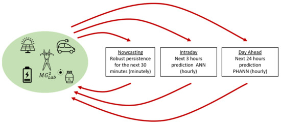
Figure 1.
Forecasting scheme and timing for photovoltaic (PV) forecasting algorithms.
In the following sections, the three methodologies are described in detail.
2.1. Day Ahead
Many approaches can be found in the literature to address the issue of providing the 24 h ahead PV power forecast and the relative power injection in the electrical grid [31]. Among all, the physical hybrid artificial neural network (PHANN) methodology was proven to provide the best results, leveraging on the adoption of the clear sky radiation [32]. The basic model is a multilayers feedforward neural network where the parameters have been set according to [33]. The PV power forecast is computed two times a day, at 11 AM and PM, when updated information is available from the weather service. A comprehensive list of the parameter provided to the PHANN both in the training and test phase can be found in [34].
2.2. Intraday
Following the prediction provided by the 24 h ahead methodology, some improvements can be performed thanks to the information collected during the plant operation: new data regarding the production of the plant and the actual measurements of environmental parameters can be beneficial to increase the model accuracy. In particular, as demonstrated in [35], they allow increasing the accuracy of the prediction of the following 3 h. Hence, this procedure is iteratively performed every hour and given the current time t, the refinement is provided for the following 3 h ().
The implemented algorithm relies on a three-layer ANN, where the hyperparameters have been optimized with a “grid search” approach. This approach allows optimizing the available parameters and hyperparameters running multiple independent simulations, varying their values in a predefined range [36]. The input parameters are the following:
- Time parameters: day of the year () and hour of the day () corresponding Timestamp to be forecast;
- Ambient parameters: global horizontal irradiation () and the Irradiation on the plane of the array () collected the previous day from the provider and already used to compute the forecast power with the 24 h ahead logic;
- Forecast power obtained with the 24 h ahead logic ();
- The last forecast error available ();
- The current measurements for the weather parameters ( and ).
2.3. Nowcasting
As shown in the literature [37], when the forecast horizon is reduced to few minutes ahead, the most promising techniques rely on statistical analysis and image processing techniques. The final purpose is to provide a useful tool to assess the PV power nowcast to be later included in a power and/or energy management system. Since image processing techniques require higher initial investment cost due to the instrumentation and is highly expensive from a computational point of view, it will not be considered in this work. The model here presented and adopted is an extension of the naïve persistence, generally employed as a benchmark for accuracy evaluation [29]. This model assumes that the future power generation at time t is the last registered value at time , being the time horizon.
As previously explained, the radiation level and hence the PV production depends on two main factors, the first one deterministic while the second one is purely stochastic. The formulation proposed in [35] addresses the first one, rewriting Equation (1) to the following:
where represents the solar altitude on the horizon, this method is referred to as Robust persistence.
3. EMS with PV Forecast Implementation
The PV forecast approaches presented in the previous section are integrated into a hierarchical EMS as the centralized control system of an MG. The EMS is suitable for a single-bus islanded electrical system, made of programmable generators, storage systems and noncontrollable RES, and it is designed to account for the production of various goods by the MG units, minimizing the daily generation cost. The hierarchical structure is subdivided into two layers to deal with the scheduling problem and the generation dispatch. In particular, the first layer oversees the daily strategic decisions based on forecasted good demands and RES generation. A predictive deterministic MILP optimization problem is employed, solved following a rolling horizon approach. The outputs of the first layer are the commitment status of the programmable generators and the planning of storage management. Real-time unbalances, and forecast errors make it necessary to contemplate correction rules that guarantee proper MG operations, handled by the second layer. Figure 2 shows the conceptual scheme behind the proposed EMS, underlining the important information exchanges among the various modules and between the EMS and the MG. Regardless of the PV forecast approach, the EMS structure remains the same. The different forecast approaches are employed to provide adjusted inputs to the first-layer optimization, which are updated accordingly with the features of the forecast method. The corresponding EMS is then named EMSDA, with day-ahead PV forecasts, EMSINT, with intraday forecast corrections, and EMSNC, with both intraday and nowcasting methods. The description of the two layers is given in the following sections; for more details, the reader can refer to previous work [12].
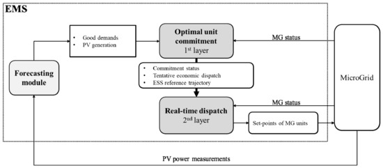
Figure 2.
Architecture and information flow of the proposed two-layer energy management systems (EMS).
3.1. First Layer Model
The purpose of the first layer is to identify the optimal unit commitment of the MG unit to ensure demand satisfaction throughout its operation at the lowest cost. The optimal commitment is obtained by the solution of an optimization problem, formulated as a deterministic mixed-integer linear program. The objective function consists in the minimization of the operating cost, made of (i) fuel consumption, (ii) startup cost of programmable units, (iii) wearing cost of storage systems and generators, (iv) penalization for unmet demands and (v) penalization for curtailment of RES generation. The operation problem that finds the optimal unit commitment based on the solution of the economic dispatch of the MG units according to the expected value of the forecasts is subjected to various constraints. Regarding the programmable generators, the constraints represent their technical limits, such as minimum and maximum output, minimum up-time and minimum downtime, and ramping limitations. Their characteristic curve, representing the relation between input and output, is expressed by a linear relation or a piecewise linear function, according to the level of approximation required. The storage systems are identified by the dynamic constraint regarding the evolution of their content, minimum and maximum capacity and the limits of exchanging the stored good with the MG (i.e., maximum charging and discharging capability). For BESS, the nonconstant efficiency of the charging and discharging process, which varies with the set-point, is expressed as a piecewise linear relationship; moreover, logical constraints are enforced to ensure non-simultaneous charge and discharge. The satisfaction of the demand is enforced by a good balance constraint that includes the virtual terms for unmet demand and RES curtailment. In order to guarantee the security margins for actual operations, the optimization accounts for spinning reserve constraints that are based on expected demand increase and expected RES generation decrease, with respect to the forecasted values: the committed generators and the storage systems must be able to satisfy the increased net demand throughout the optimization horizon. The reserve constraints of the BESS system ensure that the state of charge (SOC) is high enough to satisfy the increase of net electricity demand for the desired time interval, which is a parameter of the EMS. The mathematical formulation of the first layer model is detailed in Appendix A.
3.2. Second Layer Model
The second layer control system aims to compensate for real-time unbalances within the MG while following as close as possible the first-layer schedule (see Figure 3). The unbalances are mainly caused by forecast errors and approximation of the characteristic curves of the different units. The information obtained by the solution of the first layer gives an indication of the optimal management, provided a sufficient accuracy of the forecasts. In the proposed EMS, the commitment status of the generators is only set and updated by the first layer. On the other hand, the second layer is in charge of the real-time dispatch of the units. To avoid a greedy behavior, the main purpose of the second layer is to track the SOC evolution of the BESS foreseen by the first layer; the SOC trajectory is the translation of forecast information in terms of storage management. The tracking is achieved by a centralized PI controller. From the on-field measurements of actual SOC, the PI computes the total required variation of power output from programmable generation, complying with their ramp limitations. A linear program is then solved to optimize the power-sharing among those units. The BESS is operated under droop-control; therefore, the second layer cannot directly act on its set-point: the SOC tracking is achieved by the second layer adapting the generation of the remaining units.
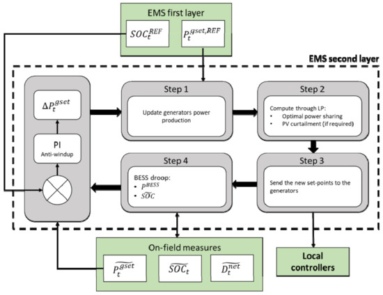
Figure 3.
Second layer flowchart.
4. Experimental Setup
The aim of this work is to perform a comparison of different PV forecast approaches used as input of the proposed EMS. First, the evaluation is performed from an experimental point of view at the MG2Lab of the Department of Energy at Politecnico di Milano.
4.1. Microgrid Description
The MG2Lab includes programmable and nonprogrammable generation units (natural gas-fired combined heat and power engine, as well as solar PV modules), different types of storage systems (electrochemical batteries, potable water and thermal storages) and various types of loads, representative of the most future on- and off-grid applications for MGMG (electricity, heating, cooling, desalination, electric bikes and electric cars). The configuration considered for this study aims at emulating the operation of a rural MG providing electricity and potable water to its users (see Figure 4). Specifically, for this analysis, the setup comprises the following units, whose technical limits are reported in Table 1:
- Two PV fields made up of monocrystalline panels (327 kWp), for a total installed capacity of 49 kWp;
- Two solar inverters of 25 kWel each coupled with the PV fields for maximum power point tracking;
- One 70 kW/67.5 kWh lithium-ion BESS;
- One 25 kWel asynchronous generator, fueled by natural gas (ICE);
- One reverse osmosis desalination system, or water purifier (WP), with an associated water tank, to increase the flexibility of potable water production;
- One back-to-back inverter (B2B) that interfaces the MG2Lab with the distribution network while decoupling voltage and frequency of the MG for off-grid operations; is used to simulate an electric load profile.

Figure 4.
MultiGood MicroGrid Laboratory (MG2Lab) single line diagram.
Figure 4.
MultiGood MicroGrid Laboratory (MG2Lab) single line diagram.


Table 1.
Technical limits of MG2Lab units in this study.
Table 1.
Technical limits of MG2Lab units in this study.
| Min. Out | Max. Out | Ramp Limit | |
|---|---|---|---|
| BESS | −70 kW | 70 kW | --- |
| ICE | 12.5 kW | 25 kW | 3 kW/min |
| WP | 650 L/h | 1000 L/h | 150 L/min |
The MG2Lab is operated in islanded mode, with the BESS operating in grid-forming mode. The BESS inverter imposes frequency (50 Hz) and voltage (400 V) to the MG, and it is operated in a droop control, acting as a slack-node for both active and reactive power. The reactive power flow has not been considered in the EMS control layers due to the limited extension of the low-voltage experimental facility, which can be considered as a single-node system. The MG is controlled by a master programmable logic controller (PLC) and 3 slave PLC, communicating the master through a PROFINET network; all the PLC are managed by the software PC WORX. The power measurements are directly acquired by the PLC networks. Concerning the BESS SOC, its estimation is evaluated by the integrated battery management system (BMS) that was provided by the BESS manufacturer; the BMS employs a combined approach based on current and voltage methods. The SOC value is continuously updated through current integration over time. To correct the measured drift caused by pure current integration, the BMS updates the SOC estimate through look-up tables and voltage measurements when certain levels are approached during the discharge phase (i.e., 60%, 40%, 20%). During the update, the SOC value is kept constant while the BESS is still discharging until its estimate matches the actual BESS content. Figure 5 provides an example of the BMS update.
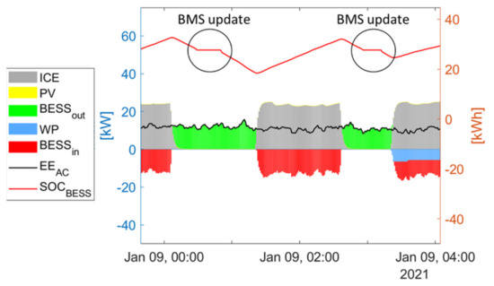
Figure 5.
Example of state of charge (SOC) measure during experimental operations: the SOC update by the battery management system is highlighted in the circled areas.
4.2. EMS Implementation
The EMS, presented in Section 3, is deployed in online software on the MG workstation. The optimization model is written in Matlab formulated through YALMIP [38] and solved with Gurobi [39], with a MIP gap set to 1%, on a computer with Intel® Core™ i9-7900X CPU @ 3.3 GHz, and an average solution time of 5 s. The two-layer structure is arranged between the workstation and the PLC, illustrated in Figure 6 and explained as follows:
- Workstation: the software corresponds to the first layer of the hierarchical EMS, thus including the forecasting and the optimization modules. They are assigned to cyclic tasks in the Matlab environment through timer objects. The first layer problem is defined over a horizon of 24 h with a resolution of 15 min, and it is solved in a rolling horizon, with an advancement time of 15 min. The forecasting module updates the PV profiles and sends the new information in synchronism with the timing of the selected forecast methods. Moreover, the Matlab software communicates with the PLC through the MODBUS interface, sending the set-point and collecting the measurements of the MG status every 20 s.
- PLC: the second layer is implemented on the PLC software since only one programmable generator is included in this setup, meaning that the proposed second layer problem is simplified, and the solution of the LP is no longer required. Thus, the PLC receives from the first layer the reference SOC and the commitment and directly computes the set-point of the programmable generators with a discretization of 100 ms, following the scheme presented in Section 3.2.

Figure 6.
EMS implementation structure.
Figure 6.
EMS implementation structure.

4.3. Case Study Definition
The case study concerns the operations of an off-grid MG, defined according to the considered MG2Lab units introduced in Section 4.1. The critical electric load curve (corresponding to the nonprogrammable loads and simulated by the B2B) was taken by the data provided by Engie-EPS [40], and the water demand profile was estimated by the NREL tool [41]. Both demands were appropriately scaled to match the production capacity of the MG2Lab units. As this study aims at addressing the effects of different PV forecast methods on MG operation, the real and the forecasted profiles of critical electricity demand and water demand are kept the same for each day of the experimental campaign. The characteristics of those demand profiles are shown in Figure 7 and Table 2. The PV forecasts and actual products will be detailed in the following subsections. The metrics here adopted to evaluate the forecast accuracy are the normalized mean absolute error (nMAE) and the normalized root-mean-squared error (nRMSE), whose definition can be found in [42], and the overall energy discrepancy between the actual production and the forecast one throughout the whole day considered.
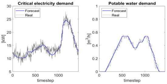
Figure 7.
Critical electricity demand and potable water demand profiles employed in this study.
Table 2.
Characteristics of demand profiles.
5. Experimental Results
This section discusses the experimental results for the comparison of the different PV forecast approaches when implemented in a deterministic EMS. In the following comparison, one PV forecast method runs on the EMS of the MG2Lab while the other two are simulated for each of the presented days.
Since the operations are performed following a rolling horizon approach, the residual content of the storage systems at the end of the simulation cannot be imposed a priori; therefore, different EMS can lead to different final storage SOC. The difference between initial and final storage content is then accounted as an equivalent fuel saving or consumption, according to the specific average consumption of the generator during the operation (in case of residual water content, the specific electricity consumption of the WP is also considered). Moreover, the experimental results are corrected considering the disregarded energy by BMS updates.
The following experimental rolling horizon operations are also compared with the operations that would be achieved by implementing a single optimization throughout the day, called EMS0. This is done to quantify the improvements that the rolling horizon approach brings in terms of reliability, checking the amount of unsatisfied demand that the implementation of EMS0 would have caused due to erroneous day-ahead forecasts. In the case of unmet electricity demand, the reported values of fuel consumption are meaningless in representing the operating cost.
5.1. Day 1–Experimental EMSDA
This subsection shows the comparison between the experimental operations of the MG2Lab performed with the day-ahead PV forecast and the simulation with intraday and nowcasting corrections, shown in Figure 8. Regarding the day-ahead forecast, an overcast day was expected from the irradiation forecast given by the provider. The considered day, though, showed two different behavior. The unexpected sunny conditions experienced in the afternoon did not meet the day-ahead forecasts. Given the erratic trend experienced in the morning, the intraday correction tended to underestimate the production for the remaining part of the day. Finally, the forecast accuracy greatly improves, further reducing the time horizon in the nowcast application with an overall reduction on all the considered metrics. The details of the dispatch are shown in Figure 9.
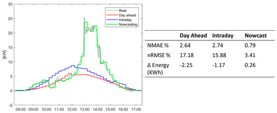
Figure 8.
PV forecasts and real profiles together with the forecast accuracy—day 1.
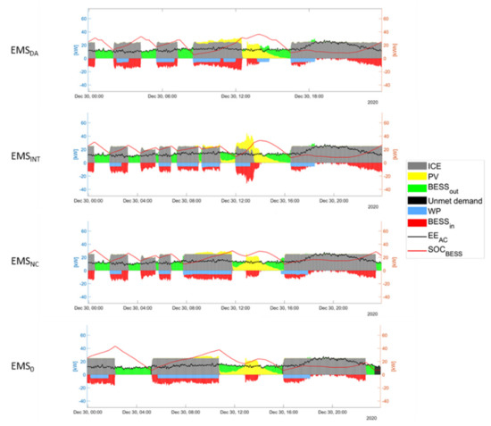
Figure 9.
Microgrid dispatch comparison—day 1 (EMSDA reflects the actual microgrid operation while the others are simulation results).
It can be noted that all the EMS decide to commit the generator since the beginning of the operation, following a cycle charge approach for most of the time, meaning that when the generator is on, it is dispatched at maximum power, using the surplus to charge the BESS and run the WP. Even though the commitment varies between EMSDA and EMSNC, the general behavior regarding BESS management is similar, consisting of a charging phase during the early hours of PV production, so to shut down the generator before the afternoon while ensuring enough energy content in the BESS to guarantee spinning reserve. The different commitment during the night is caused by the BMS updates during the experiments that disregarded 13.3 kWh during the BESS discharge phase (see Table 3). Under this circumstance, the correction obtained by the nowcasting algorithm does not influence the MG operation. Indeed, during the afternoon, only PV and BESS are in charge of balancing the electric load; therefore, even with an erroneous forecast, the dispatch is approximately the same. The EMSINT shows different behavior, starting from the first moments of PV generation. The intraday corrections, overestimating the PV production, cause an early shut down of the generator with respect to the other EMS, which is then committed around midday to comply with reserve constraints. In the meantime, the EMSINT is underestimating the PV output, but it forces to keep the generator on, according to its minimum up-time constraint. Therefore, the second layer steps in, ramping down the generator. At the end of the day, the rolling horizon approach allowed the MG to operate safely and to correctly balance the forecast errors also from an energy point of view, as the three EMS show similar fuel consumption and a decreasing value of corrected fuel consumption according to the considered corrections. Moreover, the rolling horizon approach allows avoiding 7.4 kWh of unmet electricity demand (computed by EMS0).
Table 3.
Energy summary—day 1 (the microgrid was operated with EMSDA, while the others are simulation results).
5.2. Day 2–Experimental EMSINT
This subsection shows the comparison between the experimental operations of the MG2Lab performed with intraday PV forecast and the simulation with day-ahead forecast and nowcasting corrections, reported in Figure 10. Different from the previous case, due to high variability in the solar source experienced during the day, according to the metrics, there is not an improvement deriving from the implementation of the intraday and nowcast technique. Worth noticing is that, despite the lower accuracy, in a conservative way, the intraday underestimates the production, preferable from a grid management point of view.
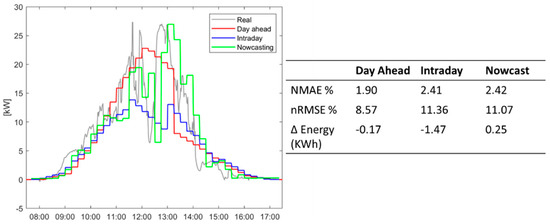
Figure 10.
PV forecasts and real profiles—day 2.
As in Figure 11, the main difference among the MG operations under the three forecast methods concerns the commitment of the generator at the beginning of the afternoon by EMSDA. During the afternoon, the day-ahead method starts overestimating the PV generation, leading to the decision of employing the WP earlier than the other two EMS. Then, a sudden underestimation of the PV production caused the commitment of the generator for security reasons. This startup is not necessary. Indeed, the BESS could be charged by PV surplus, as foreseen by EMSINT and EMSNC. In particular, the generator operates at minimum load due to second layer corrections on its set-point. This is the main reason for the higher fuel consumption by the EMSDA, as reported in Table 4. The intraday correction underestimates the PV generation, reducing the WP utilization during the afternoon, as opposed to the other EMS. This fact allowed the MG to work in safe conditions without resorting to the ICE. Overall, the three proposed EMS permit to avoid 20.2 kWh of unsatisfied electric load.
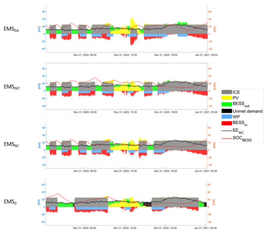
Figure 11.
Microgrid dispatch comparison—day 2. (EMSINT reflects the actual microgrid operation while the others are simulation results).
Table 4.
Energy summary—day 2 (the microgrid was operated with EMSINT, while the others are simulations results).
5.3. Day 3–Experimental EMSNC
This subsection shows the comparison between the experimental operations of the MG2Lab performed with the nowcasting method and the simulation with day-ahead forecast and intraday corrections, reported in Figure 12. As it can be inferred from the graph and the metrics table, the moving from the day-ahead forecast, a great increase in the accuracy is faced reducing the time horizon. Unexpected inaccuracy is given by the intraday model in the first hour of the afternoon, realizing a great overestimation of the available power.
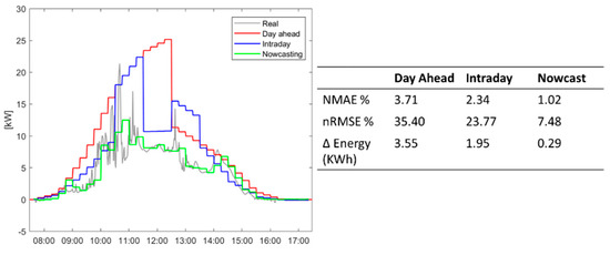
Figure 12.
PV forecasts and real profiles—day 3.
From the comparison of the forecast methods, there is a clear overestimation of the PV generation by the day-ahead method in the morning, which is then recovered with the midday update. This caused a higher utilization of the WP in the morning by the EMSDA and then a lower BESS SOC in the morning, which lead to an early startup of the generator during the day (see Figure 13). On the other hand, as the actual PV power was always lower than the electric load demand, all the EMS resort to the ICE to guarantee the spinning reserve during the afternoon. Even though the nowcasting approach corrected the erroneous forecasts, there is no clear advantage from its utilization, as the reserve constraints of the EMS already revised the commitment, ensuring safe MG operation (see Figure 12). From the point of view of EMS0, the day-ahead forecast largely overestimated the PV generation due to flawed weather forecasts; its implementation would not have guaranteed 70 kWh of electricity production, which is recovered by the other EMS, as shown in Table 5.
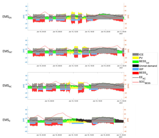
Figure 13.
Microgrid dispatch comparison—day 3 (EMSNC reflects the actual microgrid operation while the others are simulation results).
Table 5.
Energy summary—day 3 (the microgrid was operated with EMSNC, while the others are simulations results).
5.4. Discussion
The main results of the three days of operation (PV production accuracy and fuel consumptions) are reported in Table 6, suggesting that even for a simple system, as the one considered in this work with limited penetration of PV energy (around 15%), accurate PV forecast can lead to a reduction of fuel consumption while keeping safe MG operations. On the other hand, the reserve constraints in the first layer of the EMS are the main driving force for the operation scheduling, imposing the commitment decision regardless of the PV forecast method employed. This holds true because the corrections of PV forecast affect only the first timesteps of the operation, while the general schedule is based on day-ahead information for a big portion of the day, leaving little room for adjustments for the EMS that work with intraday and nowcasting refinements. Experimental results of the different cases are not comparable in terms of consumption because of the different solar radiation; however, the reliability and robustness of the methods are demonstrated. Finally, this work demonstrated the potentialities of a more accurate PV forecast on the MG management; however, no ultimate considerations can be drawn as the actual impact depends on the MG configuration, RES share and loads.
Table 6.
Summary of experimental and simulated operations.
6. Conclusions
This paper presents the implementation of a two-layer EMS on an experimental facility consisting of a multi-good off-grid MG. The first layer is based on deterministic MILP optimization for unit commitment and storage management, and the second layer is based on PI control to follow the schedule chosen by the first layer while compensating for the real-time unbalances of the MG generation. The EMS works following a rolling-horizon approach, and it is conceived to interact with a forecasting module, which adjusts the PV forecast inputs with a predefined frequency: three different forecast methodologies that combine day-ahead, intraday refinement and nowcasting models are considered. The experimental results show that the proposed EMS is able to guarantee safe MG operations with every PV forecast method; no-load shedding was required during the experiments, as opposed to the simulation results performed with a single daily optimization, which shows undesirable values of unmet electricity demand. The refinement of PV forecasts leads to higher forecast accuracy and a reduction of fuel consumption. On the other hand, its effect on MG operation is overshadowed by the spinning reserve constraints that require a minimum SOC of the BESS at the beginning of each commitment update by the first layer of the EMS, mainly due to the initial status of the MG. Indeed, the more accurate information is updated with very short (nowcasting) or small advance (intraday), while the general operation schedule, thus, the MG status, is obtained according to the day-ahead forecast for the first portion of the day. Due to this asymmetry in how the information is used in the optimization process, the PV forecast update benefits are still limited. Future work will consider more complex MG configuration and the implementation of nowcasting techniques for the second layer, in charge of the power-sharing among the units, rather than its coupling with the first layer.
Author Contributions
Conceptualization, S.P. and G.M.; methodology, S.P., A.N. and G.M.; software, S.P. and A.N.; validation, S.P. and A.N.; formal analysis, S.P. and A.N.; writing—original draft preparation, S.P. and A.N.; writing—review and editing, S.L. and G.V.; supervision, S.L. and G.M.; funding acquisition, S.L. and G.M. All authors have read and agreed to the published version of the manuscript.
Funding
This research was carried out within the PROPEHT project in collaboration with ENGIE-EPS.
Institutional Review Board Statement
Not applicable.
Informed Consent Statement
Not applicable.
Conflicts of Interest
The authors declare no conflict of interest.
Appendix A
This section presents the mathematical formulation of the optimal UC employed in the first layer of the EMS described in Section 3.1. The nomenclature for the sets, indexes, parameters, and variables used in the model is reported in Table A1.
where:
Programmable generators constraints
Storage systems constraints
Spinning reserve constraints
where:
Good balance constraints
Table A1.
Nomenclature for optimal UC model.
Table A1.
Nomenclature for optimal UC model.
| Set and Indices | |
|---|---|
| Timestep | |
| Generic MG unit | |
| MG good | |
| Programmable generator | |
| Fossil-fueled generator | |
| Generator producing/consuming good | |
| Storage system | |
| Storage system participating in good balance | |
| Non-dispatchable generator (RES unit) | |
| Non-dispatchable generator producing good | |
| Parameters | |
| Forecasted demand of good | |
| Forecasted generation of non-dispatchable generator | |
| Expected increase of demand | |
| Expected decrease of non-dispatchable generation | |
| Expected net demand for spinning reserve | |
| Minimum/maximum output of unit | |
| Ramp-up/ramp-down limit of unit | |
| Maximum ramp during startup/shut-down | |
| Minimum up-time/down-time | |
| Coefficient for linear formulation of input/output relation | |
| Generic cost coefficient | |
| Variables | |
| Commitment status of generator | |
| Startup and shut-down decisions of generator | |
| Consumption and production of generator | |
| Storage content (SOC) | |
| Bus balance for storage | |
| Charging and discharging power for storage | |
| Auxiliary binary variable for storage | |
| Unmet demand of good | |
| Curtailment of non-dispatchable generation | |
| Reserve contribution from unit | |
References
- Lasseter, R.H. MicroGrids. In Proceedings of the 2002 IEEE Power Engineering Society Winter Meeting, Conference Proceedings (Cat. No.02CH37309), New York, NY, USA, 27–31 January 2002; Volume 1, pp. 305–308. [Google Scholar]
- Hatziargyriou, N.; Asano, H.; Iravani, R.; Marnay, C. Microgrids. IEEE Power Energy Mag. 2007, 5, 78–94. [Google Scholar] [CrossRef]
- Hirsch, A.; Parag, Y.; Guerrero, J. Microgrids: A review of technologies, key drivers, and outstanding issues. Renew. Sustain. Energy Rev. 2018, 90, 402–411. [Google Scholar] [CrossRef]
- Mancarella, P. MES (multi-energy systems): An overview of concepts and evaluation models. Energy 2014, 65, 1–17. [Google Scholar] [CrossRef]
- Zia, M.F.; Elbouchikhi, E.; Benbouzid, M. Microgrids energy management systems: A critical review on methods, solutions, and prospects. Appl. Energy 2018, 222, 1033–1055. [Google Scholar] [CrossRef]
- Olivares, D.E.; Mehrizi-Sani, A.; Etemadi, A.H.; Cañizares, C.A.; Iravani, R.; Kazerani, M.; Hajimiragha, A.H.; Gomis-Bellmunt, O.; Saeedifard, M.; Palma-Behnke, R.; et al. Trends in microgrid control. IEEE Trans. Smart Grid 2014, 5, 1905–1919. [Google Scholar] [CrossRef]
- Hernandez, L.; Baladron, C.; Aguiar, J.M.; Carro, B.; Sanchez-Esguevillas, A.J.; Lloret, J.; Massana, J. A Survey on Electric Power Demand Forecasting: Future Trends in Smart Grids, Microgrids and Smart Buildings. IEEE Commun. Surv. Tutor. 2014, 16, 1460–1495. [Google Scholar] [CrossRef]
- Khan, A.A.; Naeem, M.; Iqbal, M.; Qaisar, S.; Anpalagan, A. A compendium of optimization objectives, constraints, tools and algorithms for energy management in microgrids. Renew. Sustain. Energy Rev. 2016, 58, 1664–1683. [Google Scholar] [CrossRef]
- Mazzola, S.; Astolfi, M.; Macchi, E. A detailed model for the optimal management of a multigood microgrid. Appl. Energy 2015, 154, 862–873. [Google Scholar] [CrossRef]
- Malysz, P.; Sirouspour, S.; Emadi, A. An optimal energy storage control strategy for grid-connected microgrids. IEEE Trans. Smart Grid 2014, 5, 1785–1796. [Google Scholar] [CrossRef]
- Meng, L.; Sanseverino, E.R.; Luna, A.; Dragicevic, T.; Vasquez, J.C.; Guerrero, J.M. Microgrid supervisory controllers and energy management systems: A literature review. Renew. Sustain. Energy Rev. 2016, 60, 1263–1273. [Google Scholar] [CrossRef]
- Moretti, L.; Polimeni, S.; Meraldi, L.; Raboni, P.; Leva, S.; Manzolini, G. Assessing the impact of a two-layer predictive dispatch algorithm on design and operation of off-grid hybrid microgrids. Renew. Energy 2019, 143, 1439–1453. [Google Scholar] [CrossRef]
- Valibeygi, A.; Konakalla, S.A.R.; de Callafon, R. Predictive Hierarchical Control of Power Flow in Large-Scale PV Microgrids with Energy Storage. IEEE Trans. Sustain. Energy 2020, 12, 412–419. [Google Scholar] [CrossRef]
- Luna, A.C.; Meng, L.; Diaz, N.L.; Graells, M.; Vasquez, J.C.; Guerrero, J.M. Online Energy Management Systems for Microgrids: Experimental Validation and Assessment Framework. IEEE Trans. Power Electron. 2018, 33, 2201–2215. [Google Scholar] [CrossRef]
- Polimeni, S.; Moretti, L.; Manzolini, G.; Leva, S.; Meraldi, L.; Raboni, P. Numerical and experimental testing of predictive EMS algorithms for PV-BESS residential microgrid. In Proceedings of the 2019 IEEE Milan PowerTech, Milan, Italy, 23–27 June 2019; pp. 1–6. [Google Scholar]
- Parisio, A.; Rikos, E.; Glielmo, L. A Model Predictive Control Approach to Microgrid Operation Optimization. IEEE Trans. Control Syst. Technol. 2014, 22, 1813–1827. [Google Scholar] [CrossRef]
- Hooshmand, A.; Asghari, B.; Sharma, R.K. Experimental demonstration of a tiered power management system for economic operation of grid-tied microgrids. IEEE Trans. Sustain. Energy 2014, 5, 1319–1327. [Google Scholar] [CrossRef]
- Elkazaz, M.; Sumner, M.; Thomas, D. Energy management system for hybrid PV-wind-battery microgrid using convex programming, model predictive and rolling horizon predictive control with experimental validation. Int. J. Electr. Power Energy Syst. 2020, 115, 105483. [Google Scholar] [CrossRef]
- Sachs, J.; Sawodny, O. A Two-Stage Model Predictive Control Strategy for Economic Diesel-PV-Battery Island Microgrid Operation in Rural Areas. IEEE Trans. Sustain. Energy 2016, 7, 903–913. [Google Scholar] [CrossRef]
- Wan, C.; Zhao, J.; Member, S.; Song, Y. Photovoltaic and Solar Power Forecasting for Smart Grid Energy Management. J. Power Energy Syst. 2015, 1, 38–46. [Google Scholar] [CrossRef]
- Jane, R.; Parker, G.; Vaucher, G.; Berman, M. Characterizing meteorological forecast impact on microgrid optimization performance and design. Energies 2020, 13, 577. [Google Scholar] [CrossRef]
- Multi-Goods MicroGrid Laboratory. Available online: https://www.mg2lab.polimi.it/ (accessed on 20 December 2020).
- Boyle, G. Renewable Electricity and the Grid: The Challenge of Variability; Routledge: Abingdon, UK, 2012; Volume 978-1844077892. [Google Scholar]
- Antonanzas, J.; Osorio, N.; Escobar, R.; Urraca, R.; Martinez-de-Pison, F.J.; Antonanzas-Torres, F. Review of photovoltaic power forecasting. Sol. Energy 2016, 136, 78–111. [Google Scholar] [CrossRef]
- Ulbricht, R.; Fischer, U.; Lehner, W.; Donker, H. First Steps Towards a Systematical Optimized Strategy for Solar Energy Supply Forecasting. In Proceedings of the ECML/PKDD 2013, 1st International Workshop on Data Analytics for Renewable Energy Integration, Prague, Czech Republic, 23–27 September 2013; pp. 14–25. [Google Scholar]
- Li, J.; Ward, J.K.; Tong, J.; Collins, L.; Platt, G. Machine learning for solar irradiance forecasting of photovoltaic system. Renew. Energy 2016, 90, 542–553. [Google Scholar] [CrossRef]
- Malvoni, M.; de Giorgi, M.G.; Congedo, P.M. Photovoltaic power forecasting using statistical methods: Impact of weather data. IET Sci. Meas. Technol. 2014, 8, 90–97. [Google Scholar]
- Su, D.; Batzelis, E.; Pal, B. Machine Learning Algorithms in Forecasting of Photovoltaic Power Generation. In Proceedings of the SEST 2019—2nd International Conference on Smart Energy Systems and Technologies, Porto, Portugal, 9–11 September 2019; pp. 10–15. [Google Scholar]
- Das, U.K.; Tey, K.S.; Seyedmahmoudian, M.; Mekhilef, S.; Idris MY, I.; Van Deventer, W.; Horan, B.; Stojcevski, A. Forecasting of photovoltaic power generation and model optimization: A review. Renew. Sustain. Energy Rev. 2018, 81, 912–928. [Google Scholar] [CrossRef]
- Yang, H.T.; Huang, C.M.; Huang, Y.C.; Pai, Y.S. A weather-based hybrid method for 1-day ahead hourly forecasting of PV power output. IEEE Trans. Sustain. Energy 2014, 5, 917–926. [Google Scholar] [CrossRef]
- Zheng, D.; Semero, Y.K.; Zhang, J.; Wei, D. Short-term wind power prediction in microgrids using a hybrid approach integrating genetic algorithm, particle swarm optimization, and adaptive neuro-fuzzy inference systems. IEEJ Trans. Electr. Electron. Eng. 2018, 13, 1561–1567. [Google Scholar] [CrossRef]
- Ogliari, E.; Dolara, A.; Manzolini, G.; Leva, S. Physical and hybrid methods comparison for the day ahead PV output power forecast. Renew. Energy 2017, 113, 11–21. [Google Scholar] [CrossRef]
- Dolara, A.; Grimaccia, F.; Leva, S.; Mussetta, M.; Ogliari, E. Comparison of training approaches for photovoltaic forecasts by means of machine learning. Appl. Sci. 2018, 8, 228. [Google Scholar] [CrossRef]
- Nespoli, A.; Mussetta, M.; Ogliari, E.; Leva, S.; Fernández-Ramírez, L.; García-Triviño, P. Robust 24 hours ahead forecast in a microgrid: A real case study. Electronics 2019, 8, 1434. [Google Scholar] [CrossRef]
- Leva, S.; Nespoli, A.; Pretto, S.; Mussetta, M.; Ogliari, E. PV plant power nowcasting: A real case comparative study with an open access dataset. IEEE Access 2020, 8, 194428–194440. [Google Scholar] [CrossRef]
- Pontes, F.J.; Amorim, G.F.; Balestrassi, P.P.; Paiva, A.P.; Ferreira, J.R. Design of experiments and focused grid search for neural network parameter optimization. Neurocomputing 2016, 186, 22–34. [Google Scholar] [CrossRef]
- Kumler, A.; Xie, Y.; Zhang, Y. A Physics-based Smart Persistence model for Intra-hour forecasting of solar radiation (PSPI) using GHI measurements and a cloud retrieval technique. Sol. Energy 2019, 177, 494–500. [Google Scholar] [CrossRef]
- Lofberg, J. YALMIP: A toolbox for modeling and optimization in MATLAB. In Proceedings of the 2004 IEEE International Conference on Robotics and Automation (IEEE Cat. No.04CH37508), New Orleans, LA, USA, 2–4 September 2004; pp. 284–289. [Google Scholar]
- Gurobi Optimization, LLC. Gurobi Optimizer Reference Manual; Gurobi Optimization, LLC: Beaverton, OR, USA, 2018. [Google Scholar]
- Rigovacca, O.; Polimeni, S.; Manzolini, G.; Leva, S.; Raboni, P. Analyses of electrification and battery ageing processes in a real offgrid hybrid microgrid. In Proceedings of the 2019 IEEE Milan PowerTech, Milan, Italy, 23–27 June 2019. [Google Scholar]
- Li, X.; Salasovich, J.; Reber, T. Microgrid Load and LCOE Modelling Results; NREL Data Catalog; National Renewable Energy Laboratory: Golden, CO, USA, 2018. [Google Scholar]
- Leva, S.; Mussetta, M.; Ogliari, E. PV module fault diagnosis based on micro-converters and day-ahead forecast. IEEE Trans. Ind. Electron. 2018, 66, 3928–3937. [Google Scholar] [CrossRef]


Publisher’s Note: MDPI stays neutral with regard to jurisdictional claims in published maps and institutional affiliations. |
© 2021 by the authors. Licensee MDPI, Basel, Switzerland. This article is an open access article distributed under the terms and conditions of the Creative Commons Attribution (CC BY) license (http://creativecommons.org/licenses/by/4.0/).