Thermodynamics and Machine Learning Based Approaches for Vapor–Liquid–Liquid Phase Equilibria in n-Octane/Water, as a Naphtha–Water Surrogate in Water Blends

Abstract

The prediction of phase equilibria for hydrocarbon/water blends in separators, is a subject of considerable importance for chemical processes. Despite its relevance, there are still pending questions. Among them, is the prediction of the correct number of phases. While a stability analysis using the Gibbs Free Energy of mixing and the NRTL model, provide a good understanding with calculation issues, when using HYSYS V9 and Aspen Plus V9 software, this shows that significant phase equilibrium uncertainties still exist. To clarify these matters, n-octane and water blends, are good surrogates of naphtha/water mixtures. Runs were developed in a CREC vapor–liquid (VL_Cell operated with octane–water mixtures under dynamic conditions and used to establish the two-phase (liquid–vapor) and three phase (liquid–liquid–vapor) domains. Results obtained demonstrate that the two phase region (full solubility in the liquid phase) of n-octane in water at 100 °C is in the 10⁻⁴ mol fraction range, and it is larger than the 10⁻⁵ mol fraction predicted by Aspen Plus and the 10⁻⁷ mol fraction reported in the technical literature. Furthermore, and to provide an effective and accurate method for predicting the number of phases, a machine learning (ML) technique was implemented and successfully demonstrated, in the present study.

1. Introduction

Simulation software can be typically used in the oil and gas industry to provide a quick process analysis and to facilitate engineering decisions. De Tommaso et al. [1] highlighted the importance of process simulators to build digital twins, facilitating the implementation of industry 4.0 guidelines. Usually, simulation software are used to establish the project economics, through the optimization of each process step involved [2]. For instance, to optimize the production from oil and gas fields, it is essential to have extensive knowledge of the volumetric and phase changes taking place, from the petroleum reservoir to the oil refinery [3]. When bitumen is extracted from oil sand and a naphthenic process is employed for froth treatment, the Naphtha Recovery Unit (NRU) is employed to recover naphtha from the tailings, for reuse in the process and to reduce the environmental impact of the process. This is an energy-intensive step, with environmental guidelines for naphtha recovery are required to be met [4]. Therefore, the thermodynamics for highly diluted hydrocarbon in water systems is of particular interest. While HYSYS V9 and Aspen Plus V9 software may be used with this objective in mind, the results regarding hydrocarbon/water mixtures from these simulations are not always reliable.

Hydrocarbons are separated from wastewaters before their disposal, usually by using vapor–liquid equilibrium operations. In this sense, the knowledge of the thermodynamic behavior of hydrocarbon/water systems is of importance. It is well established that the miscibility between water and hydrocarbons is limited. However, and while hydrocarbon solubility in the aqueous phase is small, it can still be an issue vis-à-vis environmental regulations and process footprint [3].

Liquids exhibit partial miscibility only when their interactions at the molecular scale display strong positive deviations from ideality. In the case of hydrocarbon/water mixtures, these interactions do not yield full liquid–liquid miscibility [5]. However, some partially miscible systems may become fully miscible at higher temperatures, with the effect of total pressure increase being negligible [5].

Water and hydrocarbons do not intermix well. Water tends to segregate from hydrocarbons as a result of the strong polar forces acting between molecules [3]. As expressed by Carlson (1996) [6], most equilibria calculations assume two phases only: vapor–liquid equilibrium (VL). However, in hydrocarbon/water blends, three vapor–liquid–liquid (VLL) phases may also contribute, with this behavior being a function of the separator operating conditions. In this respect, the accurate establishment of the number of phases (two or three phases) is critical for phase equilibrium calculations.

The selection of the proper thermodynamic method to represent hydrocarbon/water mixtures is of major importance. To accomplish this, available decision trees were described by others [1,6]. For non-ideal mixtures, however, as is the case of n-octane/water systems, the NRTL model can be used.

Jia et al. (2018) [7] investigated the separation of the n-propanol/water azeotrope, using Aspen Plus, with different thermodynamic models. According to their experimental data, n-propanol/water systems form a homogeneous azeotrope, but Aspen Plus simulations mispredicted it by calculating two liquid phases [7]. On the other hand, de Tommaso et al. (2020) [1] calculated the absence of an azeotrope for the water and acetic acid blends, using available binary parameters from the PRO/II database and the UNIQUAC model.

Moreover, Marcilla et al. (2017) [8] analyzed 25 papers with 70 cases considered for the liquid–liquid equilibrium (LLE) of ternary systems using a Non-Random Two-Liquid Model (NRTL) model. In the reported cases, 60% of the cases considered displayed phase inconsistencies in 52% of the papers reviewed. Regarding the number of phases discrepancies reported, they were assigned to (i) parameters representing partial miscibility in systems that are totally miscible; (ii) tie-line inconsistencies that do not satisfy the phase equilibrium criterion, showing meta-stable solutions and non-compliance with the iso-activity condition; and (iii) the use of mass fractions instead of molar fractions for model definition.

In Marcilla et al.’s study [8], 12 examples using Aspen Plus for the LLE data regression were described. Three of them reported inconsistencies, with the cause being assigned to the calculation algorithm. In this regard, as Marcilla et al. [8] stated, the use of unreliable parameters can create severe uncertainty, when used in chemical process simulation software. Furthermore, given this situation, Marcilla et al. [8] recommended the use of the minimization of the Gibbs energy of mixing function $\left(\mathsf{\Delta }{G}_{mix}/RT\right)$, as an additional condition to ensure the phase equilibrium prediction consistency.

Machine learning (ML) techniques have been used in chemical engineering for more than 35 years, helping to solve problems that require pattern recognition, and reasoning and decision making under complex conditions [9]. In the case of flash calculations, the phase stability test and phase splitting calculations have also been studied. From an experimental point of view, phase thermodynamic equilibrium is usually measured in experimental setups that provide a limited number of data points in manageable times. Phase equilibrium measurements for dilute hydrocarbon/water systems were made in a specially designed CREC-VL Cell were reported [10,11]. Unlike earlier experimental techniques, the implemented CREC VL Cell is operated in the dynamic mode with a temperature ramp [10,11], recording up to 10 points per second of P_mix values. This can be considered as “big data” in the context of these experiments. Big data in ML is characterized by data volume (size or scale), variety (multitype), velocity (batch or streaming), and veracity (uncertainty, quality, and accuracy) [12,13,14]. ML is about modeling data [15] and combines statistics, optimization and computer science [16]. ML gives computers the ability to learn without being explicitly programmed [17].

Schmitz et al. [18] proposed a classification methodology to solve the phase stability test, by determining the number and nature of the phases present in the ethanol/ethyl acetate/ water system, which show an heterogeneous azeotrope. They used Feedforward Neural Networks (FNN) and Probabilistic Neural Networks (PNN) trained with the data obtained from the NRTL model with literature parameters. Their model was able to correctly predict the type of equilibrium for more than 99.9% of the cases.

Poort et al. [19] studied water/methanol mixtures, using classification neural networks for the phase stability and regression networks to calculate thermodynamic properties. The data for training was generated for 101 feed composition, 500 temperatures (273–700 K), and 500 pressures (1 × 10⁴–3 × 10⁷ Pa). Overall, phase classification showed accuracy scores that were quite high (around 97%), although classification accuracy of the two-phase region was considerably lower than that of the pure liquid and vapor phase regions. Many property predictions showed good accuracy (R² > 0.95).

Kashinath et al. [20] studied the isothermal phase equilibria at 260 K and 370 K using a compositional model (3, 6, and 13 components). Data for reservoir conditions was generated by a phase diagram using isothermal negative flash calculations. The authors used relevance vector machines (RVMs) for a classification problem in order to solve the phase stability. Following this, they solved the phase split by using artificial neural networks (ANN), which predicted equilibrium K-values.

Given the above, the objectives of this work are as follows: (i) to establish the problems faced with estimating the number of phases in highly diluted octane/water mixtures when using HYSYS V9 and Aspen Plus V9, and (ii) to develop a methodology to predict the correct number of phases, using experimental data obtained in a new CREC VL Cell [10,11].

2. Approach Adopted in the Present Study

A comparison between different thermodynamic models, using HYSYS V9 or Aspen Plus V9, was first attempted through the simulation of a flash unit. Discrepancies in simulation results were noticed depending on the software used. Then the NRTL activity coefficient model was selected and implemented in Python, with the Gibbs energy of mixing function $\left(\mathsf{\Delta }{G}_{mix}/RT\right)$ being used to explain the discrepancies between HYSYS V9 and Aspen Plus V9 parameters. As well, experimental data from a CREC VL Cell and a t-test data analysis were considered to establish the 2 phase (VL equilibrium) and the 3 phase (VLL equilibrium) domains. Furthermore, machine learning methods were implemented in order to obtain an accurate classification of the phase domains, in the 80–110 °C range. Accurate classification in this range is of great importance, as it is within the NRU operation conditions.

3. Specific Strategy

An octane/water mixture can be considered as a good surrogate for naphtha/water blends. As shown in Table 1, n-Octane has properties similar to those of naphtha, which is one of the primary solvents used in bitumen processing.

Table 1. Properties for n-Octane and Naphtha.

	n-Octane	Naphtha [21]
Carbon number	8	6–13
Molecular weight (g/gmole)	114.23	145
Boiling point (°C)	125.6	65–230
Density (kg/m3)	703	781

Table 1. Properties for n-Octane and Naphtha.

	n-Octane	Naphtha [21]
Carbon number	8	6–13
Molecular weight (g/gmole)	114.23	145
Boiling point (°C)	125.6	65–230
Density (kg/m3)	703	781

HYSYS V9 and Aspen Plus V9 software contain VL and VLL equilibrium modules, which were used as a starting point for the evaluation of conventional thermodynamic models, in the present work. Water/n-octane systems have been experimentally studied in previous works [10,11]. Furthermore, and regarding n-octane–water blends, there is already a significant body of data in the technical literature, as shown in Table 2.

Table 2. Results in the Technical Literature Related to Experiments with Water/n-Octane Mixtures.

Conditions		Ref.
Temperature: 5–25 °C	Mutual solubilities.	[22]
Temperature: 0–430 °C	Mutual solubilities. Liquid–liquid equilibrium.	[23]
Temperature: 5–75 °C	Vapor–liquid equilibrium	[24]
Temperature: 0–568 °C	Vapor–liquid equilibrium	[25]
Temperature: 25 °C	Mutual solubilities	[26]
Temperature: 0–25 °C	Mutual solubilities	[27]
Temperature: 357–387 °C Pressure: 19–23 MPa	Liquid–liquid–vapor equilibrium	[28]

Table 2. Results in the Technical Literature Related to Experiments with Water/n-Octane Mixtures.

Conditions		Ref.
Temperature: 5–25 °C	Mutual solubilities.	[22]
Temperature: 0–430 °C	Mutual solubilities. Liquid–liquid equilibrium.	[23]
Temperature: 5–75 °C	Vapor–liquid equilibrium	[24]
Temperature: 0–568 °C	Vapor–liquid equilibrium	[25]
Temperature: 25 °C	Mutual solubilities	[26]
Temperature: 0–25 °C	Mutual solubilities	[27]
Temperature: 357–387 °C Pressure: 19–23 MPa	Liquid–liquid–vapor equilibrium	[28]

3.1. Materials

Distilled water was used in all experimental studies. n-Octane was obtained from Sigma-Aldrich. It has 99.0% purity and 0% water content. The molecular weight of n-octane is 114.23 g/mol, and the molecular weight of water is 18.02 g/mol.

3.2. CREC Vapor Liquid Equilibrium Cell

The Chemical Reactor Engineering Center (CREC) recently developed a CREC VL Cell which allows the measurements of VLL equilibrium (Figure 1) using a “dynamic method”, with the temperature of the cell increasing progressively, using thermal ramp of 1.22 °C/min. As a result, every run provides a large amount of vapor–liquid equilibrium data (10 Hz), with the vapor pressure data being recorded at various temperatures, every 0.01 s. Additional explanations about the cell operation are reported in [10,11]. Data obtained from this dynamic method has been validated with static measurements [10,11].

The VL Cell uses a marine type of impeller (propeller). The unit propeller helps to ensure the homogeneous mixing of the phases, providing a good heat distribution inside the CREC VL Cell. This special cell design proposed by the CREC team allows one to analyze a process sample directly, avoiding losses of light volatile components due to sample transfers.

Two thermocouples are strategically located inside the CREC VL Cell which allows measurement of both the gas and liquid phase temperatures inside the cell. These two thermocouples are connected to a temperature data acquisition box. This data acquisition box is interfaced with a USB desktop computer port. As a result, experimental data can be stored and displayed on a PC, using an Omega Temperature data acquisition software.

In addition to these features, the CREC VL Cell includes a pressure transducer which is logged into a desktop USB port. Thus, one can observe and register the changes of pressure using the installed Omega software. Hence, one should note that the instrumentation implemented into the CREC VL Cell provides accurate temperature and pressure data [10,11]. As well, the automatization of the current CREC VL Cell allows, as stated above, the gathering of large amounts of vapor pressure data per experiment, that are very valuable for VLL equilibrium simulations and modeling. Additional information regarding CREC VL Cell is provided in Appendix A.3.

4. Mathematical Formulation

4.1. Vapor–Liquid–Liquid Equilibrium Using NRTL Model

Given the issues reported in the previous sections, a NRTL activity coefficient model [29] for VLL calculations, was implemented in the present study using Python. For low pressures (close to 1 atm), as used in the NRU, an activity coefficient model was applied.

The proposed activity coefficient model involves correction factors for the chemical potential and the fugacity, accounting as well for non-ideal interactions between chemical species [5]. The activity coefficient models can be defined in terms of the excess Gibbs free energy (Equation (1)), with excess variables representing deviations from the ideal behavior.

$$\ln {\gamma }_i=\frac{{\overline{G_i}}^E}{RT}$$

(1)

The NRTL model is based on local composition theories and can be implemented using Equation (2) to Equation (4), with $g_{ij}$ representing the interaction energy and $\alpha$ being set at 0.2–0.3 as recommended and accounting for local composition variations [5,29] as follows:

$$\frac{G^E}{RT}={\displaystyle \sum }_i{x}_i\frac{{{\displaystyle \sum }}_j{\tau }_{ji}{G}_{ji}{x}_j}{{{\displaystyle \sum }}_j{G}_{ji}{x}_j}$$

(2)

$${\tau }_{ij}=\frac{g_{ij}-g_{jj}}{RT},{\tau }_{ii}=0, G_{ij}=exp\left(-\alpha {\tau }_{ij}\right)$$

(3)

$$\ln {\gamma }_i=\frac{{{\displaystyle \sum }}_j{\tau }_{ji}{G}_{ji}{x}_j}{{{\displaystyle \sum }}_j{G}_{ji}{x}_j}+{\displaystyle \sum }_j\frac{x_j{G}_{ij}}{{{\displaystyle \sum }}_k{x}_k{G}_{kj}}\left({\tau }_{ij}-\frac{{{\displaystyle \sum }}_k{x}_k{\tau }_{kj}{G}_{kj}}{{{\displaystyle \sum }}_k{x}_k{G}_{kj}}\right)$$

(4)

NRTL model parameters were obtained from Aspen Plus V9 software and from Klauck (2006) [30].

One should note as well that, the procedure for the calculation of VLL equilibrium, at isothermal and isobaric conditions, considers the coexistence of three VLL phases, as described in Figure 2 and Equations (5) and (6).

$$P_{TPR}=\sum P_i=x_1^I{\gamma }_1^I{P}_{v, 1}^{sat}+x_2^{II}{\gamma }_2^{II}{P}_{v, 2}^{sat}$$

(5)

$$y_{1,TPR}=\frac{x_1^I{\gamma }_1^I{P}_{v, 1}^{sat}}{P_{TPR}}$$

(6)

with $P_{v, \mathrm{i}}^{sat}$ representing the vapor pressure of the i component (1 for water and 2 for n-octane), ${\gamma }_{\mathrm{i}}^I$ representing the activity coefficient for phase I, and ${\gamma }_{\mathrm{i}}^{II}$ representing the activity coefficient for phase II.

Regarding the cases with two liquid phases being present, as in water and hydrocarbons, the chemical species involved included partially miscible phases. As well, given that both liquid–liquid phases contribute to vapor pressure, they form a three-phase system: two liquid phases and a single vapor phase (VLL) [5]. This “Three Phase Region Domain or (TPR)” can be represented using T_TPR and P_TPR, with all three phases (vapor–liquid–liquid) containing the various chemical species [31].

Figure 2 reports the calculation procedure for the TPR conditions, in the case of Pxy (fixed T) and Txy (fixed P) calculations. One can notice in Figure 2a that when the temperature is fixed, the establishment of a Pxy involves a direct calculation. However, in the case of calculating Txy at a set pressure (Figure 2b), the process of calculation becomes iterative, and one has to use a Newton–Raphson or a successive iteration algorithm with set objective functions.

Regarding the objective functions to be considered, these functions involve the mutual solubilities of the phases. This condition is set given the need complying with the equality of the liquid fugacities of both phases at equilibrium, and the calculation of the Three Phase Region (TPR) pressure as follows:

$$F_{obj 1, i}=\sqrt{{\left(x_i^I{\gamma }_i^I-x_i^{II}{\gamma }_i^{II}\right)}^2}$$

(7)

$$F_{obj 2}=\sqrt{{\left(P-\left(x_1^I{\gamma }_1^I{P}_{v, 1}^{sat}+x_2^{II}{\gamma }_2^{II}{P}_{v, 2}^{sat}+P_{air}\right)\right)}^2}$$

(8)

Thus, to obtain Txy or Pxy equilibrium values, the mutual solubilities at VLL equilibrium can be calculated by solving Equation (7), using the fsolve function in Python. This function is a wrapper around MINPACK’s hybrid and hybrid algorithm for solving non-linear equations [32].

Finally, the VL equilibrium can be established using Equations (9) and (10), accounting for the contribution to the vapor phase by the two components of the single liquid phase.

$$P=\sum p_i=x_1^I{\gamma }_1^I{P}_{v, 1}^{sat}+x_2^I{\gamma }_2^I{P}_{v, 2}^{sat}$$

(9)

$$y_1=\frac{x_1^I{\gamma }_1^I{P}_{v, 1}^{sat}}{P}$$

(10)

4.2. Gibbs Energy Analysis from Activity Coefficient Model

A detailed description of the thermodynamic equilibrium is essential for water/hydrocarbon mixtures. To accomplish this, three key considerations can be adopted [33]: (i) equality of chemical potentials, (ii) conservation of mass, and (iii) maximization of entropy.

One should note that while chemical potential equality is a “necessary” condition, it is not sufficient to secure solution uniqueness in phase equilibrium calculations [34]. To achieve this, the system should display a maximum entropy. One should note that at a fixed pressure and temperature, the maximization of entropy is equivalent to the minimization of the Gibbs free energy. Thus, the Gibbs free energy of mixing analysis helps to determine this condition [5].

In the case of a binary system, where the reference state of each component is a pure liquid, the Gibbs free energy of mixing for the liquid phase can be calculated, as in Equation (11). Additional details of the derivation of these equations are provided in [5]:

$$\frac{\mathsf{\Delta }{G}_{mix}^L}{RT}={\displaystyle \sum }_i{x}_i\ln \left(x_i{\gamma }_i\right)=x_1\ln \left(x_1{\gamma }_1\right)+x_2\ln \left(x_2{\gamma }_2\right)$$

(11)

With x_i representing the molar fraction of each component in the liquid phase.

Thus, to establish the change of mixing Gibbs free energy for the liquid phase as per Equation (11), one must vary the x_i values in the 0 to 1 range. In this respect, a common tangent plane criterion can be applied to multiple liquid phases as described in [5,35,36]. Furthermore, and to compare the Gibbs free energy of mixing curve for liquid and vapor phases, it is important that both phases have a common reference state [35]. In this respect, the pure component as liquid at the same temperature and pressure as the mixture, is selected as the reference state $\left(\frac{G_{i,o}^L}{RT}=0\right).$

On this basis, Equations (12) and (13) can thus be considered as applicable [34,35] for the vapor phase as follows:

$$\frac{\mathsf{\Delta }{G}_{mix}^V}{RT}={\displaystyle \sum }_i{y}_i\frac{G_{i,o}^V}{RT}+{\displaystyle \sum }_i{y}_i\ln \left(y_i\right)$$

(12)

$$\frac{G_{i,o}^V}{RT}-\frac{G_{i,o}^L}{RT}=\ln \frac{P}{P_i^{sat}}$$

(13)

Thus, given Equations (12) and (13), y_i can be varied, establishing as a result, the Gibbs free energy of mixing for the gas phase in the y_i 0 to 1 range. This Gibbs free energy of mixing phase can be also considered to be under the common tangent plane criterion as suggested in [35].

In practice however, it is always useful to know, before conducting the mixing calculations, whether the liquid–liquid blend considered yields a single liquid phase solution, or whether species in the liquid phase may split in more than one liquid phase [5]. This Gibbs free energy of mixing evaluation involves NRTL activity coefficients. This is based on an excess Gibbs energy model and can be applied at low total pressures (≤10 bar), as is the case of the system under study.

5. Results and Discussion

5.1. Issues with Available Models while Evaluating VLLE

The three-phase equilibrium (VLL) of n-octane/water systems was first considered in the present study, using Aspen Plus V9 and HYSYS V9. To accomplish this, activity coefficient models (NRTL and UNIQUAC), a Peng Robinson Cubic Equation of State and a COMThermo model were evaluated. One should note that activity coefficient models offer an alternative to models which consider equations of state for low pressure systems [5]. For the case of COMThermo, the vapor phase is modeled using the Antoine vapor pressure model and the liquid phase is modeled using the Margules activity coefficient model. For a thorough comparison between models, both models (activity coefficient and fugacity coefficient) were considered in the present study using Aspen Plus V9 and HYSYS V9 and octane/water blends.

For the simulation, a 100 kgmol/h blend with a 50% mol water/50% mol n-octane mixture was fed into a flash separator working at different temperatures from 20 to 120 °C. The bubble point pressure (vapor fraction = 0) and dew point pressure (vapor fraction = 1) were then calculated. A 3-phase separator was specified in HYSYS V9. In Aspen Plus V9, a flash3 separator was set, with water being selected as a key component in the liquid phase.

One should note that while using these models for VLLE, two dominant issues were found:

• Discrepancies between models when running with two different available software (e.g. HYSYS V9 and Aspen Plus V9).
• Inconsistency of the available thermodynamic model predictions (e.g. Aspen Plus V9) with available experimental data.

Figure 3 reports bubble point pressure calculations with Aspen Plus V9 and HYSYS V9, while the estimates for dew point pressure can be found in Appendix A.1 (Figure A1). One can see that the results from HYSYS V9 differ by a large amount as compared to those from Aspen Plus V9 (differences up to 104.66%) except when the Peng–Robinson EOS is employed (mean error = 7.98% for boiling point and 3.91% for dew point). Summary of the differences is provided in

Table 3. Comparison between HYSYS V9 and Aspen Plus V9.

Model	Boiling Point Difference	Dew Point Difference
Peng Robinson	Min: 5.67% Mean: 7.98% Max: 11.58%	Min: 1.78% Mean: 3.91% Max: 6.83%
NRTL	Min: 92.88% Mean: 99.95% Max: 104.66%	Min: 34.12% Mean: 49.96% Max: 66.45%
UNIQUAC	Min: 83.20% Mean: 86.28% Max: 90.39%	Min: 37.86% Mean: 62.98% Max: 48.89%

.

Thus, VLL results when applying HYSYS V9 software must be used with extreme caution and this given these results are indicators of phase prediction inconsistency, as will be done in the upcoming Section 5.2.

Furthermore, and while reviewing HYSYS V9 VLL results for water/n-octane streams, it was possible to identify than only the Peng–Robinson (PR) Model accounts for two liquid phases, with the activity coefficient models (NRTL and UNIQUAC), considering the octane/water stream as two totally miscible liquids. This single liquid phase misrepresentation does not agree with experimentally observed liquid–liquid phase separations as reported by Kong (2020) [10], and shows the need for developing a reliable methodology for the prediction of the number of phases of hydrocarbon/water systems.

Given the above, the proposed methodology reported here is planned to allow the software user to develop a better than “black box” model, with the user being fully aware of all equations involved. With this end, a NTRL thermodynamic model was chosen for the various calculations. This model was programmed using Python, with the Gibbs free energy analysis considered using binary interaction parameters (BIP) from HYSYS V9, Aspen Plus V9 and the technical literature [30,37]. The aim was to better models leading to two-phase simulations, predicting vapor pressures and three phases region. Finally, experimental data from the CREC VL Cell was also used, and a methodology to predict the number of phases of the n-octane/water system was proposed.

5.2. Theoretical Discussion of Model Discrepancy

The Gibbs Energy Analysis from the Activity Coefficient Model described in Section 4.2 was used to understand the differences between simulation software. Figure 4 reports the ΔG^L_mix using the NRTL model at 70 °C and 100 °C. One should note that the temperatures selected were one lower, and the other higher than the Three Phases Region (TPR) at 1 atm, as reported by Tu et al. [24]. Concerning the BIP (Binary Interaction Parameters), the ones from HYSYS V9, Aspen Plus V9, and Klauck et al. [30] were used. In the case of HYSYS V9, two cases were considered: (a) the BIPs parameters for HYSYS V9 were set at the zero default values and (b) the BIPs were estimated by HYSYS V9 assuming liquid phase immiscibility.

Figure 4 reports that the HYSYS V9 results having the BIPs set to zero, display a catenary shaped curve (in yellow), with only one anticipated liquid phase for the mixture at both 70 °C and 100 °C. One should note that the ΔG_mix/RT in HYSYS V9 is inconsistent with experimental observations where a liquid–liquid phase equilibrium is observed [10]. Furthermore, and when considering HYSYS V9 with the non-zero BIPs as reported in

Table 4. Predicted Mutual Solubilities for Water(1)/n-Octane(2) Blends at 70 °C and 100 °C in liquid phase molar fractions.

	70 °C		100 °C
BIP reference	Water in Hydrocarbon phase (x1I)	n-Octane in Aqueous phase (x2II)	Water in Hydrocarbon phase (x1I)	n-Octane in Aqueous phase (x2II)
Klauck et al. (2006) [6,29]	3.32245 × 10−3	9.1571 × 10−7	9.56125 × 10−3	9.3652 × 10−7
Aspen Plus (Python)	7.50095 × 10−3	8.1543 × 10−6	2.644388 × 10−2	2.1395 × 10−5
HYSYS (estimated BIP)	8.9570 × 10−6	0.02069	1.3065 × 10−5	0.05936
HYSYS (zero) (* one single phase)	−6.1590 × 10−10	1	−6.1590 × 10−10	1

, predicts a phase splitting behavior. Nevertheless, the ΔG_mix/RT differs significantly from the other ΔG_mix/RT calculated with Aspen Plus V9 and Klauck et al. [30] BIPs.

Furthermore, the calculation of mutual water/n-octane solubilities, assuming a single liquid phase, is considered as shown in Table 4. One can see the significant difference of BIP parameters for the various models. As expected, BIPs from HYSYS V9, when set to zero, give a trivial single-liquid phase solution which is not in agreement with experimental results [10]. Furthermore, and when Aspen Plus V9 or Klauck et al. [30] are employed, the solubility of water in the hydrocarbon phase is as expected, higher than the one for the hydrocarbon in a water phase. On the other hand, one can also observe that in the case of HYSYS V9, with non-zero estimated parameters, the predicted relative solubility is the reverse in magnitude. This means, that there is a discrepancy between the mutual solubilities obtained using the BIP default parameters of the NRTL, and the ones calculated with the HYSYS V9 method.

To address these issues, both the “unstable” and the “metastable” regions of the liquid–liquid equilibrium for a n-octane/water system were calculated, as reported in Figure 5a–d. Furthermore, and to establish the boundary between unstable and metastable regions, inflection points complying with the second derivative criteria as in (Equation (14)) were considered [5,38]. As explained by Soares et al. (1982) [39], a feed with a composition in the metastable region, may either present as a single liquid phase or alternatively may split and form two liquid phases under external perturbations.

$$\frac{d^2\mathsf{\Delta }{G}_{mix}}{d{x}_1^2}=0$$

(14)

Figure 5. Unstable and Metastable Liquid–Liquid Equilibrium Regions for a Water/n-Octane Blends using: (a,b) Klauck et al. parameters [30] and (c,d) Aspen Plus V9 parameters. Parameters reprinted with permission from Klauck, M.; Grenner, A.; Schmelzer, J. Liquid–liquid(–liquid) equilibria in ternary systems of water + cyclohexylamine + aromatic hydrocarbon (toluene or propylbenzene) or aliphatic hydrocarbon (heptane or octane). J. Chem. Eng. Data, 2006, 51, 1043–1050, doi:10.1021/je050520f. Copyright 2021 American Chemical Society.

Figure 5. Unstable and Metastable Liquid–Liquid Equilibrium Regions for a Water/n-Octane Blends using: (a,b) Klauck et al. parameters [30] and (c,d) Aspen Plus V9 parameters. Parameters reprinted with permission from Klauck, M.; Grenner, A.; Schmelzer, J. Liquid–liquid(–liquid) equilibria in ternary systems of water + cyclohexylamine + aromatic hydrocarbon (toluene or propylbenzene) or aliphatic hydrocarbon (heptane or octane). J. Chem. Eng. Data, 2006, 51, 1043–1050, doi:10.1021/je050520f. Copyright 2021 American Chemical Society.

Furthermore, it is possible to observe in Figure 5a–d, that a “stable” region boundary can be established by using a “double tangent line” (black broken line) connecting two ΔG_mix points. These “double tangent line” shared points correspond to the mutual miscibility of both phases. The double tangent condition shows the system stable state [34,40]. One should note that in the case of the “metastable” region, the temperature and model parameters that are used have an influence over the region, adding uncertainty over the mixture stability.

Figure 6 reports the VLLE at 1 atm and 89.5 °C, for the water/n-octane blends. This condition corresponds to the calculated TPR (Three Phase Region) at 1 atm. One should note that TPRs at 89.89 °C [24] and 86.76 °C [23] were previously reported. It is possible to observe, as is suggested in Figure 6a, that the tangent line now contacts the “three” ΔG_mix minima points, instead of two, with this corresponding to two liquid phases and one vapor phase condition (Three Phase Region). One can notice as well, that the “three-point tangent line” is better described by Klauck et al. [30] parameters. However, and as shown in the “close up” in Figure 6b, in practice, none of the available models present an exact three-point tangent line. This suggests that there are errors in this prediction and that a better model still needs to be developed.

Figure 7 provides a closer view of the ΔG_mix for VLLE at 70 °C, for n-octane–water blends, at low and high n-octane concentration levels, with this showing that evaluating mutual miscibility of hydrocarbon/water systems remains a challenge. In fact, for the low water molar fractions, the solubility of water in the hydrocarbon phase is described as a change of slope in the ΔG_mix. In the same way, it is possible to notice that for high water fraction regions (aqueous phase) the solubility of hydrocarbon in water experiences a flattening of the Gibbs Free energy of mixing. In this sense, the n-octane in the water mixture presents partial miscibility, which is a critical condition to be identified for environmental reasons and process optimization purposes.

Figure 7. Closer View of ΔG_mix/RT and Mutual Solubility Regions of Water/n-Octane system. The NRTL model implemented with win Aspen Plus V9 and Klauck et al. (2000) binary interaction parameters (BIP) at 70 °C. (a) highly diluted water in n-octane region, (b) highly diluted octane in water region. Note: reported data points are from [23,24].

Figure 7. Closer View of ΔG_mix/RT and Mutual Solubility Regions of Water/n-Octane system. The NRTL model implemented with win Aspen Plus V9 and Klauck et al. (2000) binary interaction parameters (BIP) at 70 °C. (a) highly diluted water in n-octane region, (b) highly diluted octane in water region. Note: reported data points are from [23,24].

However, as presented in Figure 8, when the ΔG_mix is calculated using published data at 1 atm, for the different phases [30], the need of a better prediction of number of phases is confirmed. This is given the fact that the reported technical literature experimental data points are not located at the minimum value of the Gibbs energy of mixing.

Specifically in the case of Figure 8b, the vapor phase ΔG_mix varies significant when calculated at 89.5 °C or alternatively at 89.89 °C, the experimental reported value [24]. As a result, the shared tangent line criterion does not strictly adhere in any of these two cases. In this respect, one can only agree that the availability of VLLE data at different temperatures and pressures, such as the ones provided by the CREC VL Cell, are imperative for establishing the TPR region. These data are required to obtain improved modeling of the number of phases of hydrocarbon/water mixtures.

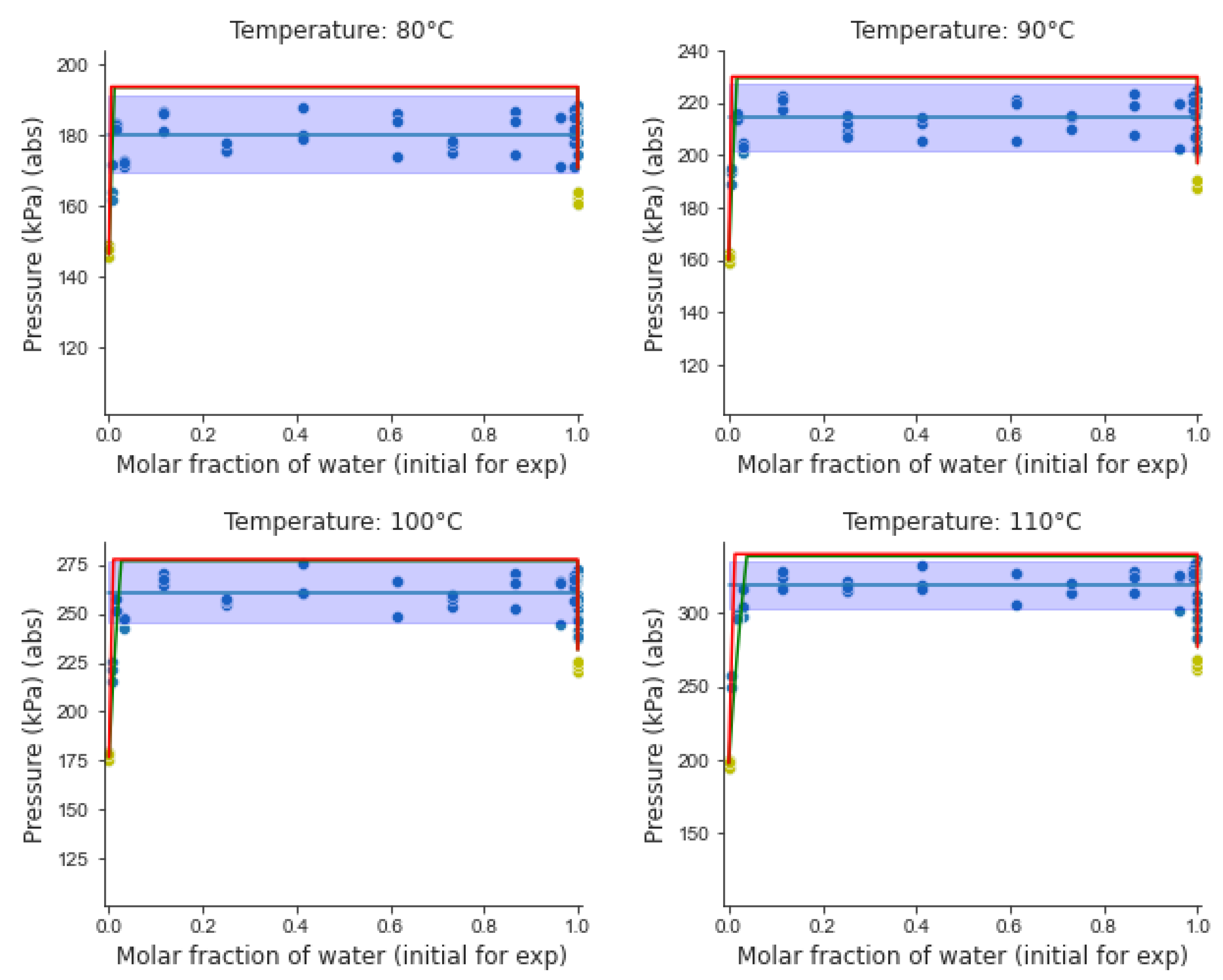
5.3. Analysis of Experimental Results

Figure 9 reports the various phase regions that one can anticipate when using n-octane/water blends. One can notice that at a given temperature, the following is expected:

(a)

Three coexisting liquid–liquid–vapor (VLL) phases with the vapor pressure remaining unchanged, while the initial water composition is varied (horizontal broken line).

(b)

Two liquids phases at higher pressures, with every phase involving highly diluted blends,

(c)

Two phases, vapor and liquid, with the liquid phase encompassing completely solubilized species.

(d)

A mixed vapor phase at low pressures.

In the present study, however, one is specially interested in the behavior described by the VLL dashed line in Figure 9, which corresponds to the Three Phase Region (TPR) and the two vapor–liquid phase domains, in the highly diluted region of a separator unit.

Regarding the experimental data considered in the present study, they are extensively described in Kong (2020) [10]. These vapor–liquid equilibrium measurements were developed at the CREC laboratory using a CREC VL Cell. These experiments were conducted using 17 different mass compositions of n-octane in water and were repeated at least three times with good reproducibility. Standard deviations for repeats were +/− 4.85 kPa in the 80–110 °C range of interest. Given the high density of the experimental data points, curves reported were obtained via linearization of data neighbors, followed by interpolation as needed for comparison of thermal levels.

Figure 10 reports the experimental points at different temperatures and octane concentrations, in the range of interest. The experimental setup considers the presence of air, as would occur in industrial operation. In that sense, the pressure of each experimental point and the models used for comparison, consider air.

Baselines with the mean values of pressure at 20% to 98%wt octane compositions were calculated and reported as blue lines in Figure 10. These baselines represent two coexisting liquid phases, as confirmed with visual observations in a Plexiglass unit [10,11]. In the same way, the blue band reports the 95% confidence intervals, calculated from the experimental data. One should also note that the red line in Figure 10 describes the fully immiscible Two Liquid Model given by (P_oct + P_w). As expected, the immiscible assumption does not represent the experimental values but rather overestimates them.

The P_mix for highly diluted octane in water (aqueous phase), and P_mix for highly diluted water in octane (hydrocarbon phase) are reported in Figure A2 and Figure A3 respectively. One can notice in both cases, there are significant P_mix reductions, with this being attributed to the solubility of highly diluted mixtures. It is also important to notice, that at 100–110 °C the highly diluted mixtures change from the TPR to the two-phase region domain. This is consistent with Figure 9, where a three-point straight line can be used to explain the presence of the three-phase region (TPR), with two liquid phases and a vapor phase being present.

Furthermore, when the NRTL model results are plotted as in Figure 11, together with the experimental data points obtained in the CREC VL Cell, similar trends for the immiscible model can be observed. Here, one can see that the TPR pressure predicted by the NRTL is higher, than the experimental values. Thus, better BIPs are needed for enhanced P_mix predictions, as is being considered in a future work, with the emphasis of the present study being on the establishment of the right number of liquid phases.

Figure 12 reports the ΔG_mix/RT calculated for n-octane/water blends at 80 °C, with those for liquid phases represented with blue lines and those for the vapor phase with a red line. Regarding the ΔG_mix/RT values, one should note that the experimental P_mix pressures were used to calculate the vapor phase, including the uncertainty related to the 95% confidence intervals (red band) using estimates from Figure 10. Furthermore, the blue bands in Figure 12 represents the ΔG_mix/RT for the liquid phases, which was calculated with the experimental temperature measurement uncertainty in the CREC VL Cell (±2 °C).

Figure 12. ΔG_mix/RT at 80 °C Using a NRTL Model and Experimental P_mix. (a) NRTL Klauck et al. [30] parameters and (b) NRTL with Aspen Plus V9 parameters. Notes: (i) Red bands represent the experimental ΔG_mix/RT uncertainty for the vapor phase, (i) Thick blue line includes the experimental ΔG_mix/RT for the liquid phases. Parameters reprinted with permission from Klauck, M.; Grenner, A.; Schmelzer, J. Liquid–liquid(–liquid) equilibria in ternary systems of water + cyclohexylamine + aromatic hydrocarbon (toluene or propylbenzene) or aliphatic hydrocarbon (heptane or octane). J. Chem. Eng. Data, 2006, 51, 1043–1050, doi:10.1021/je050520f. Copyright 2021 American Chemical Society.

Figure 12. ΔG_mix/RT at 80 °C Using a NRTL Model and Experimental P_mix. (a) NRTL Klauck et al. [30] parameters and (b) NRTL with Aspen Plus V9 parameters. Notes: (i) Red bands represent the experimental ΔG_mix/RT uncertainty for the vapor phase, (i) Thick blue line includes the experimental ΔG_mix/RT for the liquid phases. Parameters reprinted with permission from Klauck, M.; Grenner, A.; Schmelzer, J. Liquid–liquid(–liquid) equilibria in ternary systems of water + cyclohexylamine + aromatic hydrocarbon (toluene or propylbenzene) or aliphatic hydrocarbon (heptane or octane). J. Chem. Eng. Data, 2006, 51, 1043–1050, doi:10.1021/je050520f. Copyright 2021 American Chemical Society.

Thus, and as Figure 12 shows, there is an important intrinsic uncertainty when the classical, three-point tangent line criteria [35] is applied to experimental data with the available models. As was reported already when discussing Figure 8, the data from the technical literature did not exactly match the three-point tangent criteria condition. The fact, that this condition does not precisely agree with a TPR tangent line criteria, reflects the inability of the classical stability analysis to include the experimental uncertainty, when predicting the number of phases. Thus, and to address this issue more effectively, a new machine learning approach is proposed, as will be discussed in the upcoming section of this manuscript.

6. The Machine Learning Approach

Classification is one of the most commonly tasks in ML. It can be seen as converting a regression prediction problem of a target continuous variable, into a discrete function [41]. Past data (labeled items) are used to place new predictions into their respective groups or classes [41]. To establish the method reliably, standard metrics such as accuracy, true positive rate, true negative rate, precision, and a confusion matrix can be used.

In this respect, and to predict the number of phases, a classification task is implemented in the present study, with the goal of classifying the experimental data into two different equilibrium phase regions: (i) three phases (VLL) and (ii) two phases (VL). One should note that the experimental data points from the CREC VL Cell are included without averaging them, with this allowing one to incorporate the typical variations of the temperature and pressure measurements within the classification task.

The first step in this classification was to determine if the mean value of the experimental measured pressures was outside the 95% confidence interval of the VLL equilibrium baseline value.

To test this hypothesis, a t-student test was applied. This was done using the fact that the pressure baseline for highly diluted experiments displayed a difference in some liquid fraction regions. This approach allowed us to establish that the mean of the baseline was different from the experimental pressures, for highly diluted octane and highly diluted water points, with a 95% confidence interval leading to a p-value that was smaller than $\alpha =0.05$ [42].

Figure 13 and Figure 14 describe the p-values calculated for the highly diluted mixtures at different temperatures. The red line represents the $\alpha =0.05$ value while the blue line the p-values from experiments. When the experimental p-values were found to be higher than 0.05 (p-value > α), as is shown in Figure 13a for the 0.1%wt of octane in water below 85 °C, the TPR assumption was considered suitable. At temperatures above 85 °C the opposite was true, with a shift occurring from three-phases (VLL) to two-phases (VL), with octane/water being fully soluble in each other at these conditions.

On the other hand, Figure 13b,c also display the p-value for 0.25%wt and 0.5%wt of n-octane in water, with a similar transition from the TPR domain to the two-phase region, occurring at higher thermal levels of 99 °C and 108 °C, respectively.

Figure 14 considers the case of a p-value for highly diluted water in an octane blend. One can see that for 0.25%wt water in octane, there is a change from the TPR to the two-phase region at 102 °C, with the 0.1%wt water in octane blend displaying complete miscibility in the entire temperature range of interest.

Figure 15 summarizes the transition temperature for highly diluted octane in water mixtures showing a progressive increase of the transition temperature from the TPR to two-phases at initial increasing feeding separator concentrations. For instance, at concentrations in the 0.02–0.04%molar range the transition temperature rate seems faster than the one in the 0.04–0.08%molar range. Demonstrating the importance of studying the phase transitions of highly diluted hydrocarbons in water.

6.1. Classification Methodology

Four classification methods were applied to the experimental dataset from the CREC VL Cell with the objective of establishing the value of these methods to predict the number of phases in n-octane/water mixtures. To prepare the data, an identifier label was assigned according to the t-test, to experimental results as two phases or three phases (Section 5.3.). The main features involved were temperature (°C), absolute pressure (kPa, including air), z_i (mol) and phase number. The first step was to apply a min–max scaler to T and P data., z_i was already in the 0 to 1 range, and no modification was required. Furthermore, and for the phases number label, the phase class was encoded as 1 for two-Phases and 0 for three-Phases.

In terms of the classification models, logistic regression, decision tree, k-neighbors, and support vector classification from the Sklearn library in Python, were used to predict the number of phases of the experiments, available in the Temperature range of interest (80–110 °C) (refer to

Table 5. Classification Models Implemented.

Model #	Type	Hyper-Parameters	Class Weight Option
1	Logistic Regression	penalty: 12, tol: 0.0001, C: 1.0, fit_intercept: True, intercept_scaling: 1	Yes
2	Decision Tree Classifier	criterion: entropy, splitter: best, max_depth: 3, min_samples_split: 2, min_samples_leaf: 1	Yes
3	K-Neighbors Classifier	n_neighbors: 5, weights: uniform, algorithm: auto, leaf_size: 30, p: 2, metric: Minkowski	No
4	Support Vector Classifier (SVC)	C:1.0, kernel: rbf, degree: 3, gamma: scale, shrinking: True, probability: True, tol = 0.001	Yes

and Appendix A.1). One of the main challenges of this classification problem is that it consists of an imbalanced dataset, with 4056 (approximately 23%) experimental data points for the two-phase region and 13,402 data points for three-phase region as shown in Figure 16.

To address the data imbalance issue, two strategies are considered: (i) to undersample or downsize the three-Phase class so that the proportion of data to train the models is the same for both phase classes; (ii) to use a weighted algorithm, in the case of logistic regression and support vector classifier (SVC), with a class weight hyper-parameter option being used. The objective of this approach is to compare the behavior of the various models and establish which one better predicts and represents the two-Phase region.

Table 5 summarizes the four models implemented with the logistic regression, the k-neighbor classifier (KNN) and the support vector classifier (svc), using default parameters [43]. Regarding the decision tree classifier, a shallow tree (max depth = 3) with entropy as the classification criteria was considered to establish the split quality. The default hyper-parameters were selected as provided by the Scikit Learn library, to make of the model a predictive one and to demonstrate the applicability of the ML Classification.

In order to better evaluate the classification methods, 20% of the temperature data was excluded randomly from the original training dataset. This 20% of excluded data was kept aside to be included later, in the final testing dataset. After dropping these temperature data points, the remaining ones were split at 20% test data using a “train test split” function from the Sklearn library, which considers the classes ratio while performing the train splitting. Additionally, and to deal with the imbalance of the dataset, the majority class of the three phases data was randomly downsized with the idea of having two datasets with a similar class ratio.

To establish the performance of these classification models, precision, recall, and F1-score were calculated as reported in the following Equation.

$$\mathrm{precision}=\frac{TP}{TP+FP}$$

(15)

$$\mathrm{recall}=\frac{TP}{TP+FN}$$

(16)

$${\mathrm{F}}_1\mathrm{score}=\frac{2}{\frac{1}{precision}+\frac{1}{recall}}$$

(17)

Where TP refers to a true positive, TN to a true negative, FP to a false positive and FN to false negative.

Furthermore, the receiver operating characteristics (ROC) and the areas under the ROC curve (AUC) were also considered in the analysis. These parameters are commonly used in binary classifiers. ROCs plot the true positive rate (also known as recall) versus the false positive rate (FPR) [44]. It is important to note that the selected models could be calibrated, with calibrated probabilities reflecting the likelihood of true events.

6.2. Classification Models Results

In the classification analysis developed, the more abundant class (Major Class or Class 0) was randomly downsized to match the size of the less abundant class (Minor class or Class 1). Figure 17 reports the resulting confusion matrix for this strategy, with the classification report being given in

Table 6. Classification Phase Report—Strategy 1.

Logistic Regression
	Precision	Recall	F1 score
3-Phases	0.92	0.93	0.94
2-Phases	0.78	0.83	0.80
Decision Tree Classifier
	Precision	Recall	F1 score
3-Phases	1.00	0.90	0.95
2-Phases	0.75	0.99	0.85
K-Neighbors Classifier (KNN)
	Precision	Recall	F1 score
3-Phases	1.00	0.97	0.98
2-Phases	0.91	1.00	0.95
SVC
	Precision	Recall	F1 score
3-Phases	1.00	0.93	0.96
2-Phases	0.80	0.99	0.88

, and AUC and ROC results being shown in Figure 18a. It can be observed that the k-neighbors classifier and SVC presented the best results for the two-Phase case, which is the most valuable one in the present study. One can thus see that the k-neighbors classifier and SVC can predict both two-Phase and three-Phase experiments with high precision, recall and F1 scores.

Figure 18a presents the AUC-ROC curves for the first phase classification strategy. It is possible to observe that Logistic Regression is the one with the worst performance with an AUC of 0.97, with the KNN being the best one with an AUC of 0.998.

One should however, consider that under sampling (downsized sample) one phase class can bias the posterior probabilities of the classifier [45]. To address this issue, strategy 2, which uses weighted algorithms without changing the size of the testing dataset was considered. Figure 19,

Table 7. Classification Reports for Strategy 2.

Logistic Regression (penalized)
	Precision	Recall	F1 score
3-Phases	0.92	1	0.96
2-Phases	1	0.72	0.84
Decision Tree Classifier (penalized)
	Precision	Recall	F1 score
3-Phases	0.95	1.00	0.97
2-Phases	1.00	0.82	0.90
K-Neighbors Classifier (KNN)
	Precision	Recall	F1 score
3-Phases	1.00	0.99	0.99
2-Phases	0.97	0.98	0.98
SVC (penalized)
	Precision	Recall	F1 score
3-Phases	0.98	1	0.99
2-Phases	1	0.94	0.97

, and Figure 18b report the results for the confusion matrix, classification report and AUC and ROC results using Strategy 2. One can notice an improvement using the weighted algorithms, without under sampling, the KNN and weighted SVC results were able to improve for the two-Phase predictions, reducing the number of false positives and false negatives.

Given the promise of obtaining ML results for phase classification, the calibration plot for the KNN model and the weighted SVC, which represent the best models, were further validated as reported in Figure 20a,b. As a result, one can conclude that the ML model was well calibrated with the predicted probabilities corresponding closely to the expected distribution of probabilities for each class.

As well, one can notice that the KNN classifier shows near perfect calibration, with this being an improvement over the weighted SVM classifier. In addition, the KNN model presents the better results overall, and is selected for our future work. Thus, it is shown in the present study, that machine learning provides a valuable tool to accurately discriminate between two-Phase and three-Phase equilibrium regions. This prediction is critical while implementing phase equilibrium calculations, where the identification of the number of phases is a critical starting point for the flash calculations. This is achieved using to train the ML classifiers the abundant CREC VL Cell experimental data, instead of available thermodynamic models or simulation software, securing the good quality of the data considered and the adequate successful application of ML techniques. Classification models are provided in Picke format in the Supplementary Materials Section.

7. Conclusions

• It is shown that reliable models, based on fundamentals principles, are still needed to represent the number of phases, in diluted hydrocarbon in water mixtures at phase equilibria.
• It is proven that a phase stability analysis involving the Gibbs energy of mixing, can be used to explain calculation result discrepancies, in water/n-octane mixtures when using available simulation software.
• It is demonstrated that runs in a CREC VL Cell employing a dynamic technique (1.22 °C/min temperature ramp), can provide the “big data sets” required to accurately determine the fully miscible, partially miscible, and fully immiscible octane/water blend states.
• It is proven that ML models based on the obtained “big data sets” can be proposed for the prediction of the number of phases under the studied conditions, with the KNN model and the weighted SVC model, identified as the ones with best performance.

References

1. De Tommaso, J.; Rossi, F.; Moradi, N.; Pirola, C.; Patience, G.S.; Galli, F. Experimental methods in chemical engineering: Process simulation. Can. J. Chem. Eng. 2020, 98, 2301–2320. [Google Scholar] [CrossRef]
2. Banerjee, D.K. Oil Sands, Heavy Oil & Bitumen: From Recover to Refinery; PennWell Corporation: Tilsa, OK, USA, 2012. [Google Scholar]
3. Pedersen, K.S.; Christensen, P.L.; Shaikh, J.A. Phase Behavior of Petroleum Reservoir Fluids, 2nd ed.; Taylor & Francis Group, LLC: Boca Raton, FL, USA, 2015. [Google Scholar]
4. Du, J.; Cluett, W. Modelling of a Naphtha Recovery Unit (NRU) with Implications for Process Optimization. Processes 2018, 6, 74. [Google Scholar] [CrossRef] [Green Version]
5. Matsoukas, T. Fundamentals of Chemical Engineering Thermodynamics: With Applications to Chemical Processes; Pearson Education, Inc: Ann Arbor, MI, USA, 2013. [Google Scholar]
6. Carlson, E.C. Don’t Gamble With Physical Properties. Chem. Eng. Prog. 1996, 92, 35–46. [Google Scholar]
7. Jia, H.; Wang, H.; Ma, K.; Yu, M.; Zhu, Z.; Wang, Y. Effect of thermodynamic parameters on prediction of phase behavior and process design of extractive distillation. Chinese J. Chem. Eng. 2018, 26, 993–1002. [Google Scholar] [CrossRef]
8. Marcilla, A.; Reyes-Labarta, J.A.; Olaya, M.M. Should we trust all the published LLE correlation parameters in phase equilibria? Necessity of their assessment prior to publication. Fluid Phase Equilib. 2017, 433, 243–252. [Google Scholar] [CrossRef] [Green Version]
9. Venkatasubramanian, V. The promise of artificial intelligence in chemical engineering: Is it here, finally? AIChE J. 2019, 65, 466–478. [Google Scholar] [CrossRef]
10. Kong, J. Multiphase Equilibrium in A Novel Batch Dynamic VL-Cell Unit with High Mixing: Apparatus Design and Process Simulation. The University of Western Ontario, 2020. Available online: https://ir.lib.uwo.ca/etd/7283/ (accessed on 31 August 2020).
11. Escobedo, S.; Kong, J.; Lopez-Zamora, S.; de Lasa, H. Synthetic Naphtha Recovery from Water Streams: Vapor-Liquid-Liquid Equilibrium (VLLE) Studies in a Dynamic VL-Cell Unit with High Intensity Mixing. Can. J. Chem. Eng. 2021. (In Press) [Google Scholar]
12. He, Q.P.; Wang, J. Application of systems engineering principles and techniques in biological big data analytics: A review. Processes 2020, 8, 951. [Google Scholar] [CrossRef]
13. Duever, T.A. Data science in the chemical engineering curriculum. Processes 2019, 7, 830. [Google Scholar] [CrossRef] [Green Version]
14. Chiang, L.; Lu, B.; Castillo, I. Big data analytics in chemical engineering. Annu. Rev. Chem. Biomol. Eng. 2017, 8, 63–85. [Google Scholar] [CrossRef]
15. Trappenberg, T.P. Fundamentals of Machine Learning; Oxford University Press (OUP): Oxford, UK, 2019. [Google Scholar]
16. Pereira, F.C.; Borysov, S.S. Machine Learning Fundamentals. In Mobility Patterns, Big Data and Transport Analytics: Tools and Applications for Modeling; Antoniou, C., Dimitriou, L., Pereira, F., Eds.; Elsevier Inc.: Amsterdam, The Netherlands, 2019; pp. 9–29. [Google Scholar]
17. Pecht, M.G. Prognostics and Health Management of Electronics; John Wiley & Sons Ltd: Hoboken, NJ, USA, 2018. [Google Scholar]
18. Schmitz, J.E.; Zemp, R.J.; Mendes, M.J. Artificial neural networks for the solution of the phase stability problem. Fluid Phase Equilib. 2006, 245, 83–87. [Google Scholar] [CrossRef]
19. Poort, J.P.; Ramdin, M.; van Kranendonk, J.; Vlugt, T.J.H. Solving vapor-liquid flash problems using artificial neural networks. Fluid Phase Equilib. 2019, 490, 39–47. [Google Scholar] [CrossRef] [Green Version]
20. Kashinath, A.; Szulczewski, M.L.; Dogru, A.H. A fast algorithm for calculating isothermal phase behavior using machine learning. Fluid Phase Equilib. 2018, 465, 73–82. [Google Scholar] [CrossRef]
21. Naphtha (petroleum), hydrotreated heavy [MAK Value Documentation, 2010]. In The MAK-Collection for Occupational Health and Safety (eds and); Wiley-VCH: Weinheim, Germany, 2015. [CrossRef]
22. Black, C.; Joris, G.G.; Taylor, H.S. The solubility of water in hydrocarbons. J. Chem. Phys. 1948, 16, 537–543. [Google Scholar] [CrossRef]
23. Mączyński, A.; Wiśniewska-Gocłowska, B.; Góral, M. Recommended liquid-liquid equilibrium data. Part 1. Binary alkane-water systems. J. Phys. Chem. Ref. Data 2004, 33, 549–577. [Google Scholar] [CrossRef]
24. Tu, M.; Fei, D.; Liu, Y.; Wang, J. Phase Equilibrium for Partially Miscible System of Octane-Water. J. Chem. Eng. Chinese Univ. 1998, 12, 325–330. [Google Scholar]
25. Heidman, J.L.; Tsonopoulos, C.; Brady, C.J.; Wilson, G.M. High-temperature mutual solubilities of hydrocarbons and water. Part II: Ethylbenzene, ethylcyclohexane, and n-octane. AIChE J. 1985, 31, 376–384. [Google Scholar] [CrossRef]
26. Tsonopoulos, C. Thermodynamic analysis of the mutual solubilities of hydrocarbons and water. Fluid Phase Equilib. 2001, 186, 185–206. [Google Scholar] [CrossRef]
27. Polak, J.; Lu, B.C.-Y. Mutual Solubilities of Hydrocarbons and Water at 0 and 25 °C. Can. J. Chem. 1973, 51, 4018–4023. [Google Scholar] [CrossRef] [Green Version]
28. Aktiengesellschaft, B.; Ludwigshqfen, D. Fluid mixtures at high pressures IX. Phase phenomena mixtures separation and critical + water). J. Chem. Thermodyn. 1990, 22, 335–353. [Google Scholar]
29. Renon, H.; Prausnitz, J.M. Local compositions in thermodynamic excess functions for liquid mixtures. AIChE J. 1968, 14, 135–144. [Google Scholar] [CrossRef]
30. Klauck, M.; Grenner, A.; Schmelzer, J. Liquid-liquid(-liquid) equilibria in ternary systems of water + cyclohexylamine + aromatic hydrocarbon (toluene or propylbenzene) or aliphatic hydrocarbon (heptane or octane). J. Chem. Eng. Data 2006, 51, 1043–1050. [Google Scholar] [CrossRef]
31. Chien, H.H. Formulations for three-phase flash calculations. AIChE J. 1994, 40, 957–965. [Google Scholar] [CrossRef]
32. Paarsch, H.J.; Golyaev, K. A Gentle Introduction to Effective Computing in Quantitative Research What Every Research Assistant Should Know; MIT Press: London, UK, 2016. [Google Scholar]
33. Connolly, M. An isenthalpic-Based Compositional Framework for Nonlinear Thermal Simulation; Stanford University: Stanford, CA, USA, 2018. [Google Scholar]
34. Privat, R.; Jaubert, J.N.; Berger, E.; Coniglio, L.; Lemaitre, C.; Meimaroglou, D.; Warth, V. Teaching the Concept of Gibbs Energy Minimization through Its Application to Phase-Equilibrium Calculation. J. Chem. Educ. 2016, 93, 1569–1577. [Google Scholar] [CrossRef]
35. Olaya, M.D.M.; Reyes-Labarta, J.A.; Serrano, M.D.; Marcilla, A. Vapor-liquid equilibria: Using the gibbs energy and the common tangent plane criterion. Chem. Eng. Educ. 2010, 44, 236–244. [Google Scholar]
36. Jaubert, J.N.; Privat, R. Application of the double-tangent construction of coexisting phases to Any Type of Phase Equilibrium For Binary Systems Modeled With the Gamma-Phi Approach. Chem. Eng. Educ. 2014, 48, 42–56. [Google Scholar]
37. Liaw, H.J.; Chen, C.T.; Gerbaud, V. Flash-point prediction for binary partially miscible aqueous-organic mixtures. Chem. Eng. Sci. 2008, 63, 4543–4554. [Google Scholar] [CrossRef] [Green Version]
38. Baker, L.E.; Pierce, A.C.; Luks, K.D. Gibbs Energy Analysis of Phase Equilibria. Soc. Pet. Eng. J. 1982, 22, 731–742. [Google Scholar] [CrossRef]
39. Soares, M.E.; Medina, A.G.; McDermott, C.; Ashton, N. Three phase flash calculations using free energy minimisation. Chem. Engng. Sci. 1982, 37, 521–528. [Google Scholar] [CrossRef]
40. Michelsen, M.L. The isothermal flash problem. Part II. Phase-split calculation. Fluid Phase Equilib. 1982, 9, 21–40. [Google Scholar] [CrossRef]
41. Delen, D. Predictive Analytics: Data Mining, Machine Learning and Data Science for Practitioners, 2nd ed.; Pearson Education Inc.: Old Tappan, NJ, USA, 2020. [Google Scholar]
42. Sahu, P.K.; Pal, S.R.; Das, A.K. Estimation and Inferential Statistics; Springer: New Delhi, India, 2015. [Google Scholar]
43. Buitinck, L.; Louppe, G.; Blondel, M.; Pedregosa, F.; Andreas, C.M.; Grisel, O.; Niculae, V.; Prettenhofer, P.; Gramfort, A.; Grobler, J.; et al. API design for machine learning software: Experiences From the Scikit-Learn Project. arXiv 2013, arXiv:1309.0238. [Google Scholar]
44. Géron, A. Hands-On Machine Learning with Scikit-Learn, Keras, and TensorFlow, 2nd ed.; O’Reilly Media, Inc.: Newton, MA, USA, 2019. [Google Scholar]
45. Pozzolo, A.D.; Caelen, O.; Johnson, R.A.; Bontempi, G. Calibrating probability with undersampling for unbalanced classification. In Proceedings of the 2015 IEEE Symposium Series Computational Intelligence, Cape Town, South Africa, 7–10 December 2015. [Google Scholar] [CrossRef]
46. Cranganu, C.; Breaban, M.E.; Luchian, H. Artificial Intelligent Approaches in Petroleum Geosciences; Springer International Publishing: Dordrecht, The Netherlands, 2015. [Google Scholar]
47. Sinha, U.; Dindoruk, B.; Soliman, M. Prediction of CO Minimum Miscibility Pressure MMP using Machine Learning Techniques. In Proceedings of the Society of Petroleum Engineers-SPE Improved Oil Recovery Conference, Tulsa, OK, USA, 18–22 April 2020. [Google Scholar] [CrossRef]
48. Kubat, M. An Introduction to Machine Learning; Springer International Publishing: Dordrecht, The Nerthlands, 2015. [Google Scholar]
49. Kazemi, P.; Steyer, J.P.; Bengoa, C.; Font, J.; Giralt, J. Robust data-driven soft sensors for online monitoring of volatile fatty acids in anaerobic digestion processes. Processes 2020, 8, 67. [Google Scholar] [CrossRef] [Green Version]
Figure 1. Chemical Reactors Engineering Center (CREC) vapor–liquid (VL) Cell: (1) Stirring head, (2) Isolation shells, (3) Stirring hot plate, (4) Aluminum vessel, (5) VL Cell, (6) Thermofield, (7) Octane/water blend.
Processes 09 00413 g001
Figure 2. Algorithm for Three Phase Region (TPR): (a) Calculations at a fixed T and (b) Calculations at a fixed P.
Processes 09 00413 g002
Figure 3. Bubble Point Pressure Calculations with Different Thermodynamic Models for (a) HYSYS V9 and (b) Aspen Plus V9. Note: 0.5 Octane/0.5 water molar fractions.
Processes 09 00413 g003
Figure 4. Gibbs Free Energy of Mixing for a n-Octane/Water System, at Various Water Molar Fractions and Two Thermal Levels: (a) 70 °C and (b) 100 °C.
Processes 09 00413 g004
Figure 6. Vapor–Liquid–Liquid Equilibrium: (a) ΔGmix/RT including the full range of values, (b) ΔGmix/RT close-up for water/n-octane system at 1 atm and T = 89.5 °C.
Processes 09 00413 g006
Figure 8. Comparison of the Vapor ΔGmix with Available Data from the Technical Literature for (a) VLE at 99.76 °C and 1 atm and (b) VLLE at 89.5 °C and 1 atm. Note: Reported data points are from [24].
Processes 09 00413 g008
Figure 9. Schematic Description of the Two and Three Phase Regions for n-Octane/Water Blends Using the NRTL Model.
Processes 09 00413 g009
Figure 10. Experimental Pmix Results at 80 °C and 100 °C. Note: (i) The red line describes the two-phase fully immiscible model, (ii) all Pmix experimental and model derived points include the presence of air.
Processes 09 00413 g010
Figure 11. Comparison of Pmix for the NRTL Model with Experimental Data. Notes The Pmix from NRTL Aspen Plus is represented as a green horizontal line while the Pmix from the NRTL from Klauck [30] is represented as a red line. Parameters reprinted with permission from Klauck, M.; Grenner, A.; Schmelzer, J. Liquid–liquid(–liquid) equilibria in ternary systems of water + cyclohexylamine + aromatic hydrocarbon (toluene or propylbenzene) or aliphatic hydrocarbon (heptane or octane). J. Chem. Eng. Data, 2006, 51, 1043–1050, doi:10.1021/je050520f. Copyright 2021 American Chemical Society.
Processes 09 00413 g011
Figure 13. T-student test for Highly Diluted Octane in Water Experiments (a) 0.1%wt octane, (b) 0.25%wt octane, (c) 0.5%wt octane.
Processes 09 00413 g013
Figure 14. T-student test for Highly Diluted Water in Octane Experiments (a) 99.75%wt octane, (b) 99.9%wt octane.
Processes 09 00413 g014
Figure 15. Temperature Change from the TPR to the Two Phase Region (highly diluted octane in water) (a) mass percentage, (b) mol percentage.
Processes 09 00413 g015
Figure 16. Distribution of Three Phase (liquid–liquid–vapor) and Two Phase (Liquid–vapor) Data Available.
Processes 09 00413 g016
Figure 17. Confusion Matrix for the Tested Classification Models using Strategy 1.
Processes 09 00413 g017
Figure 18. Area under the ROC curve (AUC) and receiver operating characteristics (ROC)—Results for Strategies (a) 1 and (b) 2.
Processes 09 00413 g018
Figure 19. Confusion Matrix for Strategy 2.
Processes 09 00413 g019
Figure 20. Calibration for (a) KNN and (b) SVC Models.
Processes 09 00413 g020