Article

Modeling the Influence of Temperature, Light Intensity and Oxygen Concentration on Microalgal Growth Rate

by
Ignacio López Muñoz
1 and
Olivier Bernard
1,2,*
1
BIOCORE, Université Côte d’Azur, INRIA, BP 93, 06902 Sophia Antipolis Cedex, France
2
Sorbonne Université, CNRS, UMR 7093, Laboratoire d’Océanographie de Villefranche, F-06230 Villefranche-sur-Mer, France
*
Author to whom correspondence should be addressed.
Processes 2021, 9(3), 496; https://doi.org/10.3390/pr9030496
Submission received: 8 February 2021 / Revised: 24 February 2021 / Accepted: 2 March 2021 / Published: 9 March 2021
(This article belongs to the Special Issue Modelling and Optimal Design of Complex Biological Systems)

Abstract

:
Dissolved oxygen plays a key role in microalgal growth at high density. This effect was so far rarely quantified. Here we propose a new model to represent the combined effect of light, oxygen concentration and temperature (LOT-model) on microalgae growth. The LOT-model introduces oxygen concentration in order to represent the oxidative stress affecting the cultures, adding a toxicity term in the expression of the net growth rate. The model was validated with experimental data for several species such as Chlorella minutissima, Chlorella vulgaris, Dunaliella salina, Isochrysis galbana. It successfully predicted experimental records with an average error lower than 5.5%. The model was also validated using dynamical data where oxygen concentration varies. It highlights a strong impact of oxygen concentration on productivity, depending on temperature. The model quantifies the sensitivity to oxidative stress of different species and shows, for example, that Dunaliella salina is much less affected than Chlorella vulgaris by oxidative stress. The modeling approach can support an optimization strategy to improve productivity, especially for managing high oxygen levels.

1. Introduction

Microalgae are photosynthetic microorganisms that use sunlight to fix carbon dioxide. Some species store large amounts of triacylglycerol, which can be converted into biodiesel [1]. This potential has motivated many research studies in the past decade [2]. Microalgae are also known for their capacity to produce long chain polyunsaturated fatty acids with positive effects on human health [3]. They can also be a source of pigments and antioxidants for the cosmetic, pharmaceutical and food markets. Algal products are not currently in widespread use, largely due to their high production cost [4]. Optimizing this process, to enhance productivity and reduce cost is therefore a major issue. Light and temperature are the two main factors affecting productivity, especially in outdoor cultivations where they are generally not controlled. Irradiance is often too high in comparison with the photosynthetic capacity and this leads to photosaturation, and even photoinhibition [5]. Temperature has an analogous effect [6]. A higher temperature increases cell enzymatic activity and favors growth. However, when reaching a critical temperature some proteins start to denature, especially those involved in photosystems and electron transport chain, impacting cell metabolism [7] and eventually inducing cell mortality [8].
Stress due to oxygen oversaturation has been so far less studied, despite its negative effect on growth. At high concentration, O2 can compete with CO2 for RuBisCo, the key enzyme in the Calvin cycle. This so-called photorespiration leads to glycolate production instead of the glyceraldehyde 3-phosphate expected at the output of the Calvin cycle [9].
Moreover, at high light, the large amount of produced oxygen combined with the fluxes of photons and of electrons generated in Photosystem II strongly enhances the rate of reactive oxygen species (ROS) formation [10,11]. ROS leads to organelle dysfunction, alteration of cell structures, protein, and membrane damage [12]. High ROS concentration means a strong oxidative stress, and further cell mortality. For these very different reasons, oxygen has been shown to reduce specific growth rate and therefore reduce productivity [4].
The development of a mathematical model is a great opportunity to optimize the production process, and better control the growth conditions to avoid critical regimes where productivity drops. The objective of this work is to extend existing models and better quantify the coupled effect of light, temperature and oxygen concentration on microalgal growth rate. There are several models which have been developed to account for both light and temperature effects [13,14], but none of them independently describe the impact of oxygen.
The effect of light conditions has been represented by several types of models, see Béchet et al. [15] for a review. Light impact, when accounting for photoinhibition is generally described by two main models. The Steel model is based on an exponential function representing both activation by light and photoinhibition after a certain threshold [16]. Haldane kinetics, derived from the model of Eilers and Peeters [5], is also often used. The reparametrized Haldane model, as suggested by Bernard and Rémond [13], is more convenient to calibrate:
μ N I = μ max I I + μ max α I I opt 1 2
where α is the initial slope of the light response curve in m 2 s · µ mol 1 d 1 .   I and I opt are the irradiance as a variable, and the one for which growth is maximal (with respect to light), respectively, in μ mol . m 2 s 1 . μ max   is the maximum growth rate, in d 1 , for the optimal irradiance at T opt in °C.
The suitable models for representing temperature impact on microalgal growth are reviewed in [17]. The so-called cardinal temperature model with inflexion (CTMI) is a convenient way of representing the impact of temperature on growth [18]. It is widely used for bacteria and has demonstrated to be also accurate for microalgae and cyanobacteria [13]. The Hinshelwood model [19] is more mechanistic, since it represents the net growth rate ( μ N ) as the difference between two terms: growth ( μ ) and deactivation ( m ) processes, where each term follows an Arrhenius’s behavior:
μ N T = μ T m T = A 1 e E 1 R T A 2 e E 2 R T
where E 1 and E 2 are activation energies for the growth and death processes, respectively in J · mol 1 . A 1 and A 2 are the intensity of each process (dimensionless). R is the universal gas constant in J · K 1   mol 1 . The maximum temperature for growth, after which the net growth rate μ N T becomes negative is denoted   T max . The optimal temperature is the temperature at which μ N T reaches its maximum value. Grimaud et al. [17] showed that the Hinshelwood model accurately represents temperature impact on growth. However, calibration of the Hinshelwood model is challenging. In the following we propose a calibration strategy supported by the simpler CTMI model.
For moderate ranges of light and temperature, the interactions between them have been shown to stay temperate and, in terms of modeling, they are generally represented by products of two terms representing each effect [13]. The coupling becomes marked at low temperature and high light [17], where dramatic photoinhibition may occur which is not accounted for in nowadays modeling, and it is better represented in the model we propose.
The paper aims to represent the combined effect of light, oxygen concentration and temperature on microalgae growth to account for the oxidative stress affecting the cultures. The model was validated with experimental data for several species and it shows a strong impact of oxygen concentration on productivity, depending on temperature. The paper is organized as follows. In Section 2 we introduce the LOT-model quantifying the toxicity of oxygen on growth rate. Afterwards, the dynamical effect of oxygen production on biomass is presented. A calibration strategy is then proposed. In Section 3 we assess and discuss the prediction capability of the model using five different species. Model validity is then tested under dynamical conditions. Finally, a quantification of the sensitivity to oxygen concentration is proposed.

2. Model Development

2.1. Representing Growth and Toxicity Rates

The objective of the mathematical model is to support an optimization strategy and to guide the trade-off between growth rate and oxygen concentration along with operating conditions such as temperature and light intensity.
The idea behind the LOT-model is to couple the Haldane model to represent the light impact and the Hinshelwood model for the temperature effect. Additionally, we explicitly include the effect of oxygen in the deactivation term, in order to represent its toxicity. We propose to rewrite the inactivation rate in Equation (2) of Hinshelwood’s model to account for oxidative stress, which is assumed to be related to oxygen concentration:
m =   A 2 O 2 e E 2 R T = A m e E m R 1 T 1 T 0     · 1 + K m O 2 O 2 + n
where the term K m O 2 / O 2 + n   represents the microalgal sensitivity to the oxygen concentration in relation to a reference value O 2 + . The exponent n represents the action of the oxidative stress. Parameter K m shows how sensitive the microalgae is to oxidative stress. A more sensitive species is characterized by a higher K m and therefore a higher toxicity in the presence of oxygen.
Equation (3) represents a higher oxidative stress at higher oxygen concentration, and the subsequent cell toxicity. This model is supported by the results of Serra-Maia et al. [8], who observed a decrease in net growth rate for enhanced oxygen in the medium. They showed that it was mainly the result of an increase in mortality for Chlorella vulgaris.
Finally, the LOT-model combines the Haldane model for light and the Hinshelwood model with oxygen deactivation, and predicts the balance between growth and toxicity (gross growth rate):
μ G I , T , O 2 = μ m a x I I + μ m a x α I I o p t 1 2 · A G e E G R 1 T 1 T 0     A m e E m R 1 T 1 T 0     · 1 + K m O 2 O 2 + n
For constant oxygen concentration, the model is a standard Hinshelwood model, because the term K m O 2 / O 2 + n   is constant. For O 2   lower than O 2 + , the effect of oxygen remains weak. Since the Hinshelwood model and the CTMI model have quite similar behaviors, at constant or low oxygen concentrations, the LOT model will also behave similarly to the model of Bernard and Rémond [13].

2.2. Dynamic Modeling

Oxygen concentration in a photobioreactor is rarely constant and evolves together with the biomass and its activity. To accurately represent the impact of oxygen, a dynamical model is then required to quantify the evolution of the cell biomass (whose concentration is denoted x , in mg   L 1 ) along with oxygen. The differential equations describing the dynamics of the biomass in a high-density reactor is written in Equation (5):
d x d t = μ ¯ G I 0 , T , O 2 x R u x
where respiration rate R u represents the decrease in mass due to carbon loss by respiration, in day 1 . I 0 is the incident light, in μ mol . m 2 s 1 . μ ¯ G I 0 , T , O 2 is the average gross growth rate in the reactor, accounting for light gradient, as it is detailed later on. The net growth rate in the reactor is then given by μ ¯ G I 0 , T , O 2 R u . For cultures at high density (roughly speaking this means biomasses larger than 100 mg of dry weight per L), it is recommended to account for the light gradient in the computation of the average growth rate [20]. Indeed, the cells do not receive the same amount of light, depending on their distance to the illuminated surface of the reactor. Assuming a Lambert–Beer exponential decrease of light irradiance I ( μ mol   m 2 s 1 ) with depth z (m) its expression is shown in Equation (6):
    I z = I 0   · e k x z
where I 0 is the irradiance at the surface, and 𝑘 is the light extinction coefficient (in m 2 g ). The growth rate is computed by averaging μ G I z in the reactor volume. For a planar geometry of the reactor (for example in a high rate pond), it can be rewritten as Equation (7):
μ ¯ G I 0 = 1 L 0 L μ G I z d z = 1 k x L I L I 0 μ G I I d z
where L is the depth of the pond. Note that Equation (7) demonstrates that μ ¯ G I 0 is the average of the growth yield in the reactor irradiance range. If μ G I follows Haldane kinetics as in Equation (1), the final expression can be analytically computed as is shown in Equation (8), and also for more complicated geometries [21]:
μ ¯ G I 0 = 2 μ m a x k x L Δ arctan γ I 0 arctan γ I L
with Δ = 4 μ m a x α I opt 1 , assuming Δ > 0 and γ I = 2 μ m a x α I opt Δ I I opt 1 + 1 Δ .
The dynamics of oxygen, in a batch photobioreactor, results from the balance between production by photosynthesis, loss with gas exchange and respiration, as in Equation (9):
d O 2 d t = k o · μ ¯ G * I 0 x k L a   O 2 O 2 * R O 2 T x
The oxygen transfer rate k L a   represents the volumetric mass transfer coefficient for oxygen ( day 1 ). The yield of oxygen production is k o in mg   O 2 mg   x 1 . R O 2 T represents the respiration rate (in mg   O 2 · L 1 d 1 mg   x 1 ), which is an Arrhenius term, R O 2 exp E m R 1 T 1 T 0     and O 2 * is the solubility of oxygen which depends on temperature and salinity, in mg   O 2 · L 1 [22]. Note that, in Equation (9), μ ¯ G * does not depend on temperature to account for the uncoupling between the light and dark reactions in photosynthesis, so its expression corresponds to Eq (8). The dark reaction is enzymatic and temperature sensitive, while the light reaction is photochemical and has a weak dependency on temperature.

2.3. Parameter Estimation

Experimental data for model validation are extracted from a set of studies with various species carried out under different conditions. Table 1 summarizes the culture conditions for each study. Depending on the experimental studies, the growth rate was assessed as a function of temperature or as a function of light (Table 1).
As most publications did not measure the oxygen concentration, we had to provide an estimate. For example, in order to make the calibration of the data collected in [23] and [24] (growth rate as a function of light intensity), we assumed that oxygen concentration was similar to the one measured in [25] and it was considered that 135% of the saturation value was reached. The value of O 2 + was taken as the value of oxygen solubility at the experimental temperature [22]. Regarding the data of [8], oxygen was recomputed from the measured growth rate.
The first calibration stage consists of a static calibration using data sets where net growth rate was measured for different conditions of light and/or temperature. Calibration of the Hinshelwood model is challenging, due to the extreme sensitivity of its parameters. We proceeded in two stages: first, with a calibration through a template based on the simpler and easy-to-calibrate CTMI model. Once the CTMI model was calibrated, we replaced the experimental data by the fit given by the CTMI model, for a larger range of temperatures (see Appendix A for details). The strategy of calibration is shown in Figure 1.
The reparametrized Haldane model (Equation (1)) was straightforwardly fit to the growth rate records as a function of light intensity, and parameters μ m a x , α   and   I opt were derived.
The study of [6], with dissolved oxygen measurements, was used for adjusting K m and   n to the data (see Table 2).
For advanced dynamic calibration, the data in [25] were used to fit growth dynamics to measurements of biomass and oxygen along time.
Parameter identification was carried out minimizing the following objective function in Equation (10), i.e., the residues between model and data:
J θ =   i = 1 n   x e x p , i x s i m , i 2 σ x 2 + f o · j = 1 m O 2 e x p , j O 2 s i m , j 2 σ O 2 2
where θ is the vector containing all the parameters to be adjusted. Variables y e x p , j and y s i m , j are the experimental and simulated values, respectively ( x for biomass and
O 2 for dissolved oxygen concentration, with, respectively, n and m data points), σ x 2 and σ O 2 2   are the associated standard deviations. Finally, f o is the relative weight given to the oxygen fit with respect to the biomass fit. The value of f o = 25 met a trade-off, to account for the more frequent oxygen measurements.
The objective of the calibration procedure is to find a set of parameters minimizing the fitting error given by Equation (10). Each optimization was carried out using Matlab® (R2018b) function nlinfit based on the Levenberg–Marquardt nonlinear least squares algorithm [27].

2.4. Model Validation

The model was validated with the data of Li et al. [25] (for the data set with light intensity of 60 μ molm 2 s 1 ) which were not used for calibration (see Table 1).
Two criteria were taken into consideration to validate the model. Firstly, Equation (11) was used to quantify the relative prediction error between the experimental data and simulation, which must be less than 10%.
error =   1 n i = 1 n   x e x p , i x s i m , i x e x p , i
Secondly, we performed a statistical analysis adapted from [28], meaning two-sample t-test for equal means, which considers unpaired data and two samples with different variances and independent data. The aim is to answer the question whether the estimated values are significantly different in comparison with experimental data. The null hypothesis H 0 :   β ^ s i m =   β ^ e x p was tested, where β ^ s i m   and β ^ e x p are the mean values of the simulated and experimental data, respectively. The statistical test was estimated as shown in Equation (12), where N s i m   and N e x p   are the sample sizes and s s i m 2 and s e x p 2 are the sample variances. Therefore, the null hypothesis is rejected if T   >   t 1 α / 2 , ν   where t 1 α / 2 , ν is the critical value of the t-distribution with ν degrees of freedom (see Equation (13)) and, in this context, α is the significance level, taken as 0.05.
T = β ^ sim     β ^ exp s sim 2 N sim + s exp 2 N exp
ν = s s i m 2 / N s i m   + s e x p 2 / N e x p 2 s s i m 2 N s i m 2 / N s i m 1 + s e x p 2 N e x p 2 / N e x p 1

3. Results and Discussion

3.1. Static Growth Model as a Function of Temperature and Light

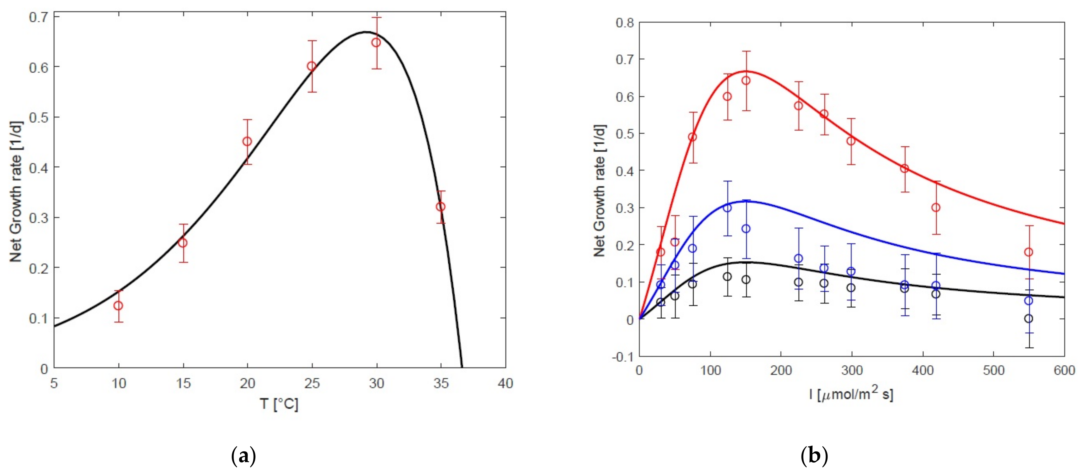
The parameters for each species obtained from the model calibration phase can be found in Table 2, reflecting different responses to light and temperatures. For Chlorella minutissima and Isochrysis galbana the fit was carried out with K m = 0.203 , reflecting the fact that experiments were performed at low oxygen concentrations and therefore with limited oxygen stress. The model was able to accurately describe the impact of the incident light intensity and temperature on net growth rate of Chlorella minutissima (data from [23]) and Isochrysis galbana (data from [24]), as shown in Figure 2 and Figure 3, respectively. It efficiently represented the net growth rate of Chlorella minutissima versus light intensity for different temperatures (10, 30 and 35°C) along with net growth rate versus temperature for   I   =   140   µ mol . m 2 s 1 . The estimation of the optimal temperature is 29.3 °C (assuming low oxygen concentrations) which agrees with the 30°C found by Aleya et al. [23]. Note that light response is better predicted for a range of temperatures closer to T o p t (Figure 2).

3.2. Growth in Dynamical Conditions

The LOT-model efficiently represents the influence of incident light intensity and temperature on net growth for different microalgae species. Here we discuss the model performance when oxygen dynamics is simultaneously predicted, using Equations (6) to (9).
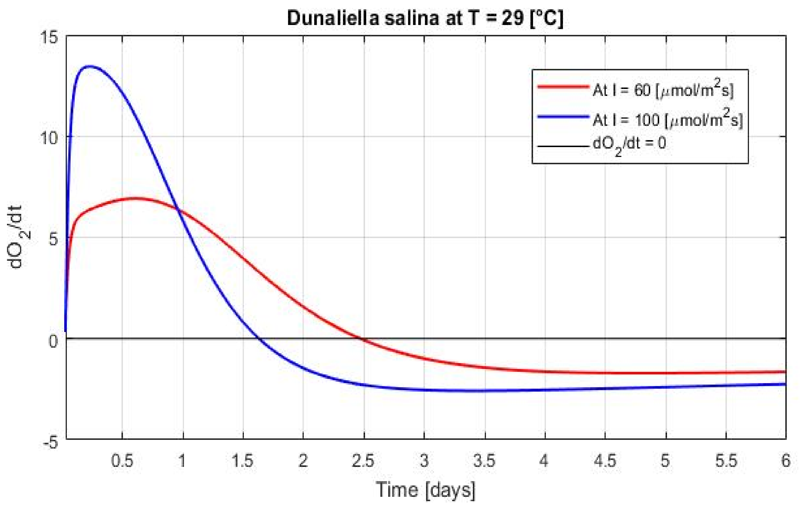
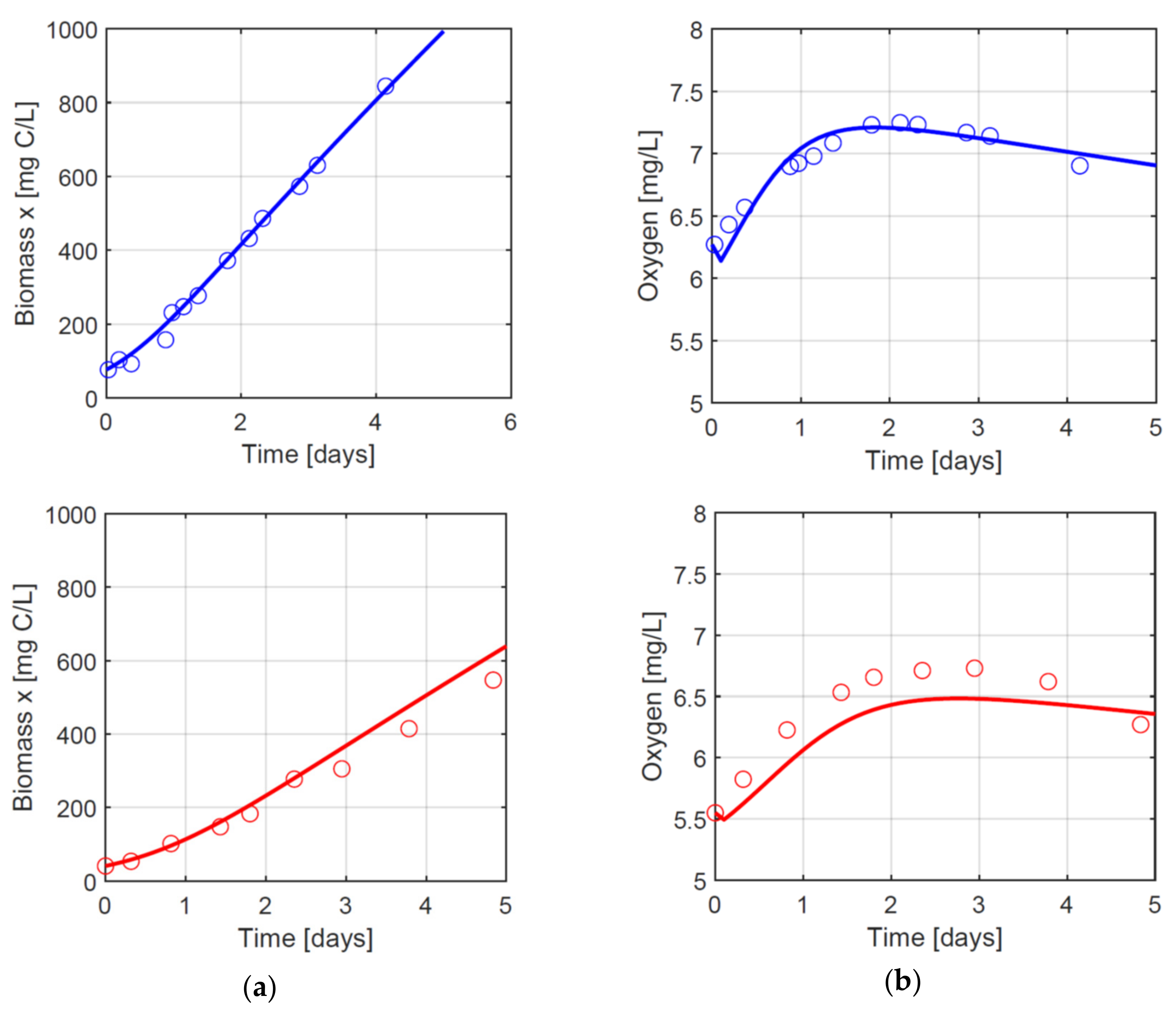
Li et al. [25] exposed Dunaliella salina to two different light intensities and recorded at the same time cell density and oxygen concentration. Simulations of LOT-model under these dynamical conditions are shown in Figure 4 and the parameters can be found in Table 2 and Table 3. The model accurately predicts the dynamics of oxygen concentration and biomass for   100   µ mol   m 2 s 1 . The average model relative error for biomass and oxygen are 6.8% and 1.1%, respectively. Figure 4 shows the abrupt oxygen drop after 3 days. It is worth remarking that our model captures this feature, due to the balance between oxygen production and gas exchange. Indeed, when computing the oxygen derivative d O 2 / d t , it turns out that its sign changes when oxygen reaches its maximum (see Figure 4 and Appendix B for details): net growth rate progressively decreases while the available light is attenuated by the increasing biomass. As a consequence, photosynthesis at the reactor scale slows down. The reduction in oxygen production is simultaneously due to the increase in oxygen concentration, mechanically reducing the growth rate. When growth rate decreases down to a certain threshold, the terms of exchange and respiration eventually dominates and finally oxygen drops.
To assess the prediction capability of the LOT-model, we consider as validation data set the experiment from [25] for I   =   60   µ mol   m 2 s 1 , which were not used in the validation phase. As it is shown in Figure 4, the model accurately predicts the dynamics of oxygen concentration and biomass, with average relative errors of 3.1% and 9.4%, respectively.

3.3. Impact of Oxygen on Response to Temperature

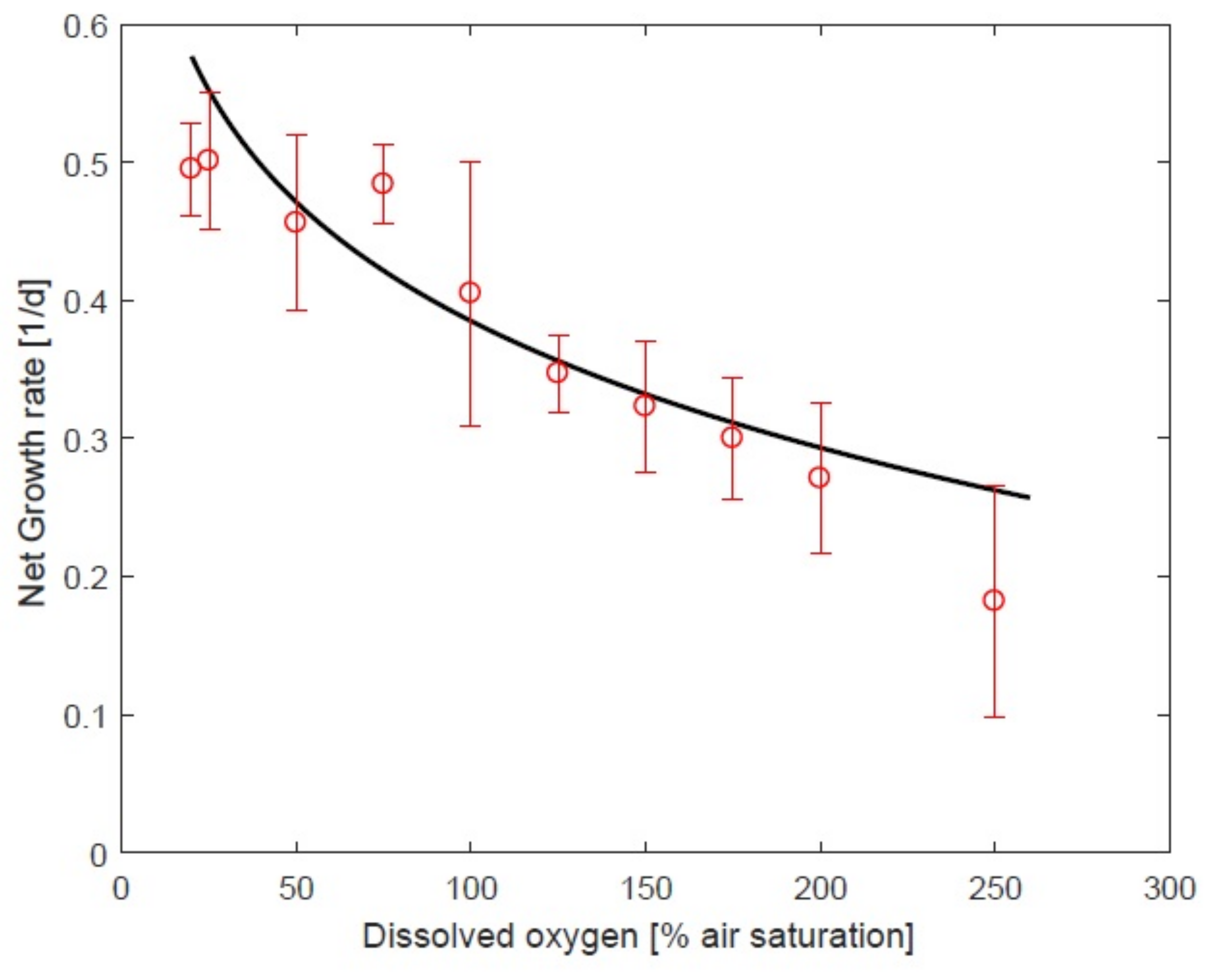
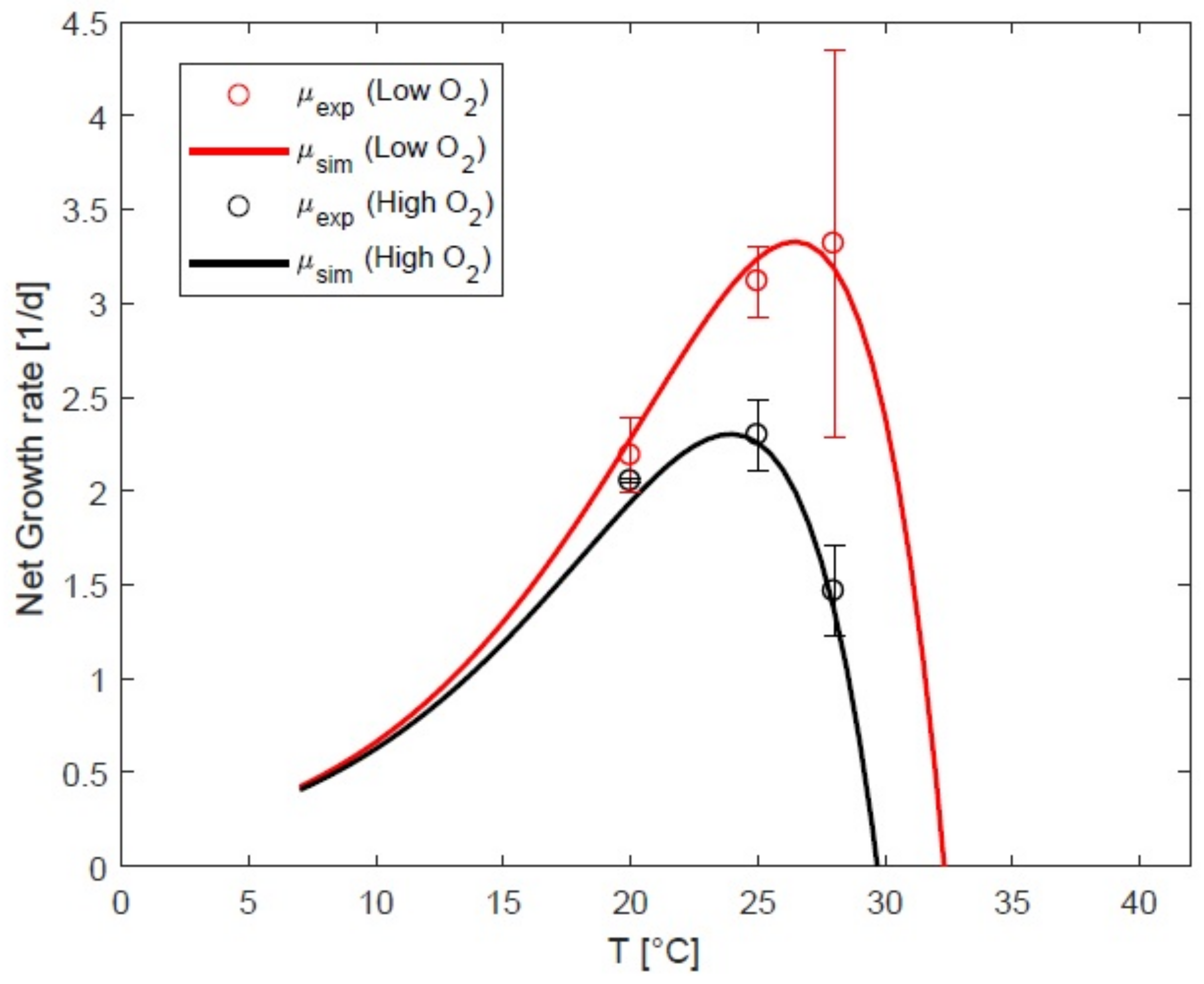
Figure 5 presents the model fit with the growth rate of Nannochloropsis sp. (CCAP 211/78) measured in [26] for different oxygen concentrations. It illustrates how the model successfully predicts the growth rate decrease when oxygen concentration increases. It is noteworthy that in situations with high O 2 concentrations, the range of temperatures where the microalgae can grow becomes narrower, with a decrease in T o p t and T m a x . This is clearly illustrated for Chlorella vulgaris in Figure 6 (4% average error at low oxygen concentration and 4.6% at high concentration). Under higher oxidative stress, lower net growth rates are reached. As a remarkable consequence, the optimal temperature shifted between the two conditions from 24 ± 2.4 to 26.5 ± 3.5°C and µ o p t   decreased from 3.3 to 2.3 day 1 .

4. Discussion

4.1. Impact of Oxygen the Growth Rate

We computed the growth rate of Chlorella vulgaris at different light intensities and temperatures for a constant level of oxygen concentration. Figure 7 simulates how the maximum reachable growth rate is affected for O 2 levels ranging from 100% to 500%. The light response curve presents a lower initial slope (see Appendix C for simulations) and a reduced maximum growth rate. This is a clear sign that the presence of a high level of oxygen strongly reduces the photosynthetic efficiency, even at low light. A similar pattern appears with temperature, where higher levels of oxygen reduce the maximal achievable growth rate. The model highlights the shift in the temperature response for higher oxygen concentrations, with the consequent reduction in the cardinal temperatures T o p t and T m a x together with the maximum growth rate. The oxidative stress hinders microalgae growth with a stronger effect at higher temperatures. It reveals that oxygen may indeed play a strong role in photobioreactors dynamics, and that oxygen must be stripped to better cope with higher temperatures.

4.2. Sensitivity to Oxidative Stress

The LOT-model can also be used to detect an oxidative stress during growth. For example, in Figure 6 for Chlorella vulgaris grown in a photobioreactor at high oxygen concentration, the ratio O 2 / O 2 + T deduced from the observed growth reduction is estimated to be 371.7 ± 17.1%. For O 2   at 300% of saturation, the optimal µ is 0.79 day 1 at T = 27.7 °C and I = 620   µ mol   m 2 s 1 . Let us define the sensitivity to oxidative stress (SOE) as Equation (14):
SOE = µ I , T , O 2 low   µ I , T , O 2 high   µ I , T , O 2 low   · 100
Considering O 2 low   = 100 % and O 2 high   = 400 % , representing a situation with limited oxygen production or strong oxygen outgassing and high oxygen concentration typical of a bioreactor at high light. Computation of S O E for Chlorella vulgaris, demonstrates a marked sensitivity to oxygen with S O E   =   41.4 % . Dunaliella salina turns out to be remarkably less sensitive to oxidative stress with S O E   =   0.01 % . Indeed, Dunaliella salina is known for its ability to resist to oxidative stress [31], probably because of the large amount of β-carotene it can store. Carotenoids are accessory light-harvesting pigments which play a key role for energy dissipation by nonphotochemical quenching and function as ROS scavengers [32].

4.3. Calibration of Hinshelwood’s Model

The Hinshelwood model has the advantage of explicitly including a deactivation term. The LOT-model uses this opportunity to represent oxygen toxicity through both mortality and growth reduction due to photorespiration. This term is a loss for the microalgal growth rate, and its accurate quantification points out a margin of progress for the optimization process. However, it includes two phenomena of very different nature. On the one hand, mortality has a deeper impact since dead biomass will stay in the reactor during a few retention times and will not regrow. As a result, it will contribute to shadowing the living cells. On the other hand, glycolate production by photorespiration is a loss for the cells which do not fix any carbon, while they reduce the oxygen level of the medium. However, cells will grow again later on when lower oxygen concentrations are reached. The ability to explicitly represent this deactivation term makes a large difference for growth modeling compared to a CTMI model. However, calibrating the Hinshelwood model is challenging, due to an extreme sensitivity to the parameter values. The reason for this is that the model includes a difference of two exponential functions, and accurate values for A G , E G , A m ,   and E m are required. Little changes on the model parameters deeply affect the model predictions. For example, in the dynamic modeling (see Section 3.2) of Dunaliella salina, increasing by 1% the value of A G , upsurged by 1100% the error for the biomass and by 448% the error for oxygen. There are similar sensitivities with E G , A m and E m . With the proposed calibration methodology, the LOT-model calibration is however straightforward and turns out to be very robust, despite this inherent sensitivity of the Hinshelwood model.

4.4. Predicting and Reducing Oxidative Stress

Some species are more sensitive to oxidative stress, and their optimal growth conditions i.e., T o p t and I o p t are deeply affected by oxygen concentration. Cultivating these species must then be associated with a strategy for controlling oxygen. The model can efficiently help managing the level of oxygen and reducing inhibition. The threshold where the excess of O 2 in the medium must be removed from the medium can be identified thanks to the model. It would then trigger a dedicated outgassing procedure, such as increasing aeration or mixing rates. An optimal control strategy with a feedback loop based on O 2 monitoring will thus reduce the periods of oxidative stress and eventually increase productivity. The Model Predictive Control strategy proposed in [33], which doubled the microalgae productivity during summer, could be extended to account for oxygen accumulation, especially with the purpose of anticipating oxygen accumulation at low temperature or at high photosynthesis rate.
Adapting the microalgae to high oxygen concentration could be another strategy to avoid a productivity decrease because of oxidative stress. Bonnefond et al. [34] carried out a long-term selection experiment and eventually increased the temperature range for which growth is possible. A continuous selection pressure could adapt microalgae to conditions with higher oxygen levels.

5. Conclusions

The LOT-model proves to accurately fit several experimental data sets at equilibrium or in dynamical conditions with an average error lower than 5.5%. It reveals that oxygen may indeed play a strong role in microalgae productivity. Since oxygen concentration in the medium is directly (solubility) or indirectly (photosynthesis) related to temperature and light, it becomes clear that this parameter must be monitored more attentively and systematically along the cultures.
Additional experiments are now necessary to further validate the model in a broader range of oxygen concentrations including experiments with both light/dark periods and periodic temperature fluctuations, which are closer to realistic scenarios of industrial exploitation of microalgae.
The LOT-model will support advanced control strategies to reduce the productivity losts due to oxygen accumulation. But it might reveal even more useful to manage algae cultured in closed photobioreactor systems, for which oxygen concentrations can reach very high concentrations [35].

Author Contributions

O.B and I.L.M. designed the model. I.L.M. developed the Matlab code and performed the calibration and simulations, O.B. assessed the respective results. I.L.M. wrote the manuscript with constant feedback from O.B. In general, all authors provided critical feedback and helped shape the research, analysis and manuscript. All authors have read and agreed to the published version of the manuscript.

Funding

This research was funded by the BIOMSA project from French environmental and energy management agency (ADEME).

Institutional Review Board Statement

Not applicable.

Informed Consent Statement

Not applicable.

Data Availability Statement

Not applicable.

Acknowledgments

This work has been carried out in the framework of the BIOMSA project supported by the French environmental and energy management agency (ADEME).

Conflicts of Interest

The authors declare no conflict of interest.

Appendix A

The CTMI model includes four parameters, each of them with a biological significance, which makes it straightforward to calibrate:
T min : Represents the temperature below which the growth is zero, in °C.
T max : Represents the temperature above which the growth is zero, in °C.
μ opt : Represents the maximal growth rate, in   day 1 .
T opt : Represents the temperature at which the growth rate reaches the maximal, in °C.
Therefore, the functions that predicts the growth rate μ max between T min and T max is:
μ max = 0                                         f o r   T < T min μ opt · ϕ T             f o r   T min < T < 0                                         f o r   T > T max T max
where
ϕ T = T T max T T min 2 T opt T min T opt T min T T opt T opt T max T opt + T min 2 T

Appendix B

In mathematical terms: As d O 2 / d t < 0 , and according to Equation (9) this is equal to k o · μ ¯ N I 0 , O 2 x k l a O 2 O 2 * R O 2 x < 0 · k o · μ ¯ N I 0 , O 2 x < k l a O 2 O 2 * + R O 2 x . In Figure A1 it is shown when there is a change from positives to negatives values of d O 2 / d t .
Figure A1. Variation on the rate of oxygen production in Dunaliella salina at 29   ° C .  
Processes 09 00496 g0a1
Production is higher during the first days, then curves change the sign, which means a decrease in the curve oxygen production versus time.

Appendix C

Figure A2 shows how the light yield α changes for Chlorella vulgaris at different oxygen concentrations (the simulation was done at T = 25 °C).
Figure A2. Variation on the initial slope of the light response curve in Chlorella vulgaris at 25   ° C .
Processes 09 00496 g0a2

References

  1. Wijffels, R.H.; Barbosa, M.J. An outlook on microalgal biofuels. Science 2010, 329, 796–799. [Google Scholar] [CrossRef] [PubMed] [Green Version]
  2. Bernard, O. Hurdles and challenges for modelling and control of microalgae for CO2 mitigation and biofuel production. J. Process. Control. 2011, 21, 1378–1389. [Google Scholar] [CrossRef]
  3. Guedes, A.C.; Meireles, L.A.; Amaro, H.M.; Malcata, F.X. Changes in lipid class and fatty acid composition of cultures of Pavlova lutheri, in response to light intensity. J. Am. Oil Chem. Soc. 2010, 87, 791–801. [Google Scholar] [CrossRef]
  4. Sousa, C.; De Winter, L.; Janssen, M.; Vermuë, M.H.; Wijffels, R.H. Growth of the microalgae Neochloris oleoabundans at high partial oxygen pressures and sub-saturating light intensity. Bioresour. Technol. 2012, 104, 565–570. [Google Scholar] [CrossRef] [PubMed]
  5. Eilers, P.H.C.; Peeters, J.C.H. A model for the relationship method is easy to implement, is less expensive than the between light intensity and the rate of photosynthesis in phytoplankton. Ecol. Model. 1988, 42, 199–215. [Google Scholar] [CrossRef]
  6. Béchet, Q.; Laviale, M.; Arsapin, N.; Bonnefond, H.; Bernard, O. Modeling the impact of high temperatures on microalgal viability and photosynthetic activity. Biotechnol. Biofuels 2017, 10, 1–11. [Google Scholar] [CrossRef]
  7. Ras, M.; Steyer, J.-P.; Bernard, O. Temperature effect on microalgae: A crucial factor for outdoor production. Rev. Environ. Sci. Biotechnol. 2013, 12, 153–164. [Google Scholar] [CrossRef] [Green Version]
  8. Serra-Maia, R.; Bernard, O.; Goncalves, A.; Bensalem, S.; Lopes, F. Influence of temperature on Chlorella vulgaris growth and toxicity rates in a photobioreactor. Algal Res. 2016, 18, 352–359. [Google Scholar] [CrossRef]
  9. Foyer, C.H.; Bloom, A.J.; Queval, G.; Noctor, G. Photorespiratory metabolism: Genes, Mutants, energetics, and redox signaling. Annu. Rev. Plant Biol. 2009, 60, 455–484. [Google Scholar] [CrossRef]
  10. Murata, N.; Takahashi, S.; Nishiyama, Y.; Allakhverdiev, S.I. Photoinhibition of photosystem II under environmental stress. Biochim. Biophys. Acta Bioenerg. 2007, 1767, 414–421. [Google Scholar] [CrossRef] [Green Version]
  11. Pospíšil, P. Enzymatic function of cytochrome b559 in photosystem II. J. Photochem. Photobiol. B Biol. 2011, 104, 341–347. [Google Scholar] [CrossRef]
  12. Takeda, T.; Yokota, A.; Shigeoka, S. Resistance of photosynthesis to hydrogen peroxide in algae. Plant Cell Physiol. 1995, 36, 1089–1095. [Google Scholar] [CrossRef]
  13. Bernard, O.; Rémond, B. Validation of a simple model accounting for light and temperature effect on microalgal growth. Bioresour. Technol. 2012, 123, 520–527. [Google Scholar] [CrossRef] [PubMed]
  14. Bernard, O.; Mairet, F.; Chachuat, B. Modelling of microalgae culture systems with applications to control and optimization. In Tissue Engineering III: Cell—Surface Interactions for Tissue Culture; Portner, R., Kasper, C., Witte, F., Eds.; Springer International Publishing: Geneva, Switzerland, 2015; Volume 153, pp. 59–87. [Google Scholar]
  15. Béchet, Q.; Shilton, A.; Guieysse, B. Modeling the effects of light and temperature on algae growth: State of the art and critical assessment for productivity prediction during outdoor cultivation. Biotechnol. Adv. 2013, 31, 1648–1663. [Google Scholar] [CrossRef] [PubMed]
  16. Steele, J.H.; Baird, I.E. Further relations between primary production, chlorophyll, and particulate carbon. Limnol. Oceanogr. 1962, 7, 42–47. [Google Scholar] [CrossRef]
  17. Grimaud, G.M.; Mairet, F.; Sciandra, A.; Bernard, O. Modeling the temperature effect on the specific growth rate of phytoplankton: A review. Rev. Environ. Sci. Biotechnol. 2017, 16, 625–645. [Google Scholar] [CrossRef]
  18. Rosso, L.; Lobry, J.R.; Flandrois, J.P. An unexpected correlation between cardinal temperatures of microbial growth high-lighted by a new model. J. Theor. Biol. 1993, 162, 447–463. [Google Scholar] [CrossRef]
  19. Hinshelwood, C.N. Kinetics of the Bacterial Cell; Oxford University Press: London, UK, 1946. [Google Scholar]
  20. Huisman, J.; Weissing, F.J. Light-limited growth and competition for light in well-mixed aquatic environments: An elementary model. Ecology 1994, 75, 507–520. [Google Scholar] [CrossRef] [Green Version]
  21. Martínez, C.; Mairet, F.; Bernard, O. Theory of turbid microalgae cultures. J. Theor. Biol. 2018, 456, 190–200. [Google Scholar] [CrossRef] [Green Version]
  22. Sherwood, J.; Stagnitti, F.; Kokkinn, M.J.; Williams, W.D. Dissolved oxygen concentrations in hypersaline waters. Limnol. Oceanogr. 1991, 36, 235–250. [Google Scholar] [CrossRef]
  23. Aleya, L.; Dauta, A.; Reynolds, C.S. Endogenous regulation of the growth-rate responses of a spring-dwelling strain of the freshwater alga, Chlorella minutissima, to light and temperature. Eur. J. Protistol. 2011, 47, 239–244. [Google Scholar] [CrossRef] [PubMed]
  24. Lin, Y.-H.; Chang, F.-L.; Tsao, C.-Y.; Leu, J.-Y. Influence of growth phase and nutrient source on fatty acid composition of Isochrysis galbana CCMP 1324 in a batch photoreactor. Biochem. Eng. J. 2007, 37, 166–176. [Google Scholar] [CrossRef]
  25. Li, J.; Xu, N.S.; Su, W.W. Online estimation of stirred-tank microalgal photobioreactor cultures based on dissolved oxygen measurement. Biochem. Eng. J. 2003, 14, 51–65. [Google Scholar] [CrossRef]
  26. Raso, S.; Van Genugten, B.; Vermuë, M.; Wijffels, R.H. Effect of oxygen concentration on the growth of Nannochloropsis sp. at low light intensity. Environ. Biol. Fishes 2011, 24, 863–871. [Google Scholar] [CrossRef] [Green Version]
  27. Horton, R.L.; Seber, G.A.F.; Wild, C.J. Nonlinear regression. J. Mark. Res. 1990, 27, 244–245. [Google Scholar] [CrossRef]
  28. Sadino-Riquelme, M.C.; Rivas, J.; Jeison, D.; Hayes, R.E.; Donoso-Bravo, A. Making sense of parameter estimation and model simulation in bioprocesses. Biotechnol. Bioeng. 2020, 117, 1357–1366. [Google Scholar] [CrossRef] [PubMed]
  29. Edwards, K.F.; Thomas, M.K.; Klausmeier, C.A.; Litchman, E. Light and growth in marine phytoplankton: Allometric, taxonomic, and environmental variation. Limnol. Oceanogr. 2015, 60, 540–552. [Google Scholar] [CrossRef] [Green Version]
  30. Schwaderer, A.S.; Yoshiyama, K.; Pinto, P.D.T.; Swenson, N.G.; Klausmeier, C.A.; Litchman, E. Ecoevolutionary differences in light utilization traits and distributions of freshwater phytoplankton. Limnol. Oceanogr. 2011, 56, 589–598. [Google Scholar] [CrossRef]
  31. Murthy, K.C.; Vanitha, A.; Rajesha, J.; Swamy, M.M.; Sowmya, P.; Ravishankar, G.A. In vivo antioxidant activity of carotenoids from Dunaliella salina—A green microalga. Life Sci. 2005, 76, 1381–1390. [Google Scholar] [CrossRef] [PubMed]
  32. Frank, H.A.; Young, A.; Britton, G.; Cogdell, R.J. The photochemistry of carotenoids. In Advances in Photosynthesis and Respiration; Sharkey, T.D., Eaton-Rye, J., Eds.; Springer Science and Business Media: Secaucus, NJ, USA, 1999; Volume 8. [Google Scholar]
  33. De-Luca, R.; Bezzo, F.; Béchet, Q.; Bernard, O. Exploiting meteorological forecasts for the optimal operation of algal ponds. J. Process. Control. 2017, 55, 55–65. [Google Scholar] [CrossRef]
  34. Bonnefond, H.; Grimaud, G.; Rumin, J.; Bougaran, G.; Talec, A.; Gachelin, M.; Boutoute, M.; Pruvost, E.; Bernard, O.; Sciandra, A. Continuous selection pressure to improve temperature acclimation of Tisochrysis lutea. PLoS ONE 2017, 12, e0183547. [Google Scholar] [CrossRef] [PubMed] [Green Version]
  35. Ugwu, C.; Aoyagi, H.; Uchiyama, H. Photobioreactors for mass cultivation of algae. Bioresour. Technol. 2008, 99, 4021–4028. [Google Scholar] [CrossRef] [PubMed]
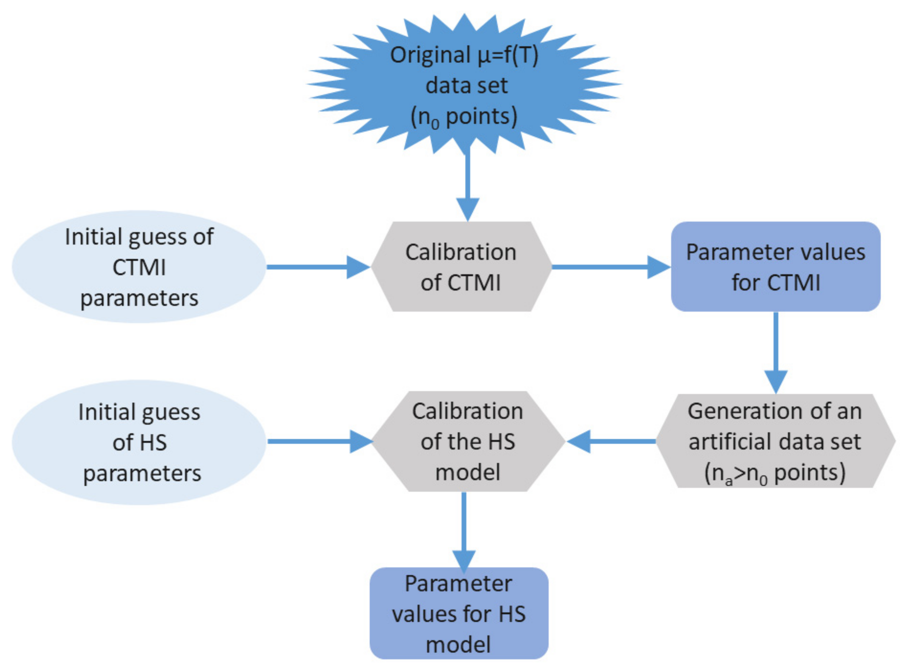
Figure 1. Algorithm for calibrating Hinshelwood’s model.
Processes 09 00496 g001
Figure 2. Model calibration at different temperatures and irradiances, with Chlorella minutissima. Experimental values (circles) and simulations (continuous lines). (a) Growth rate at I   =   140   µ mol · m 2 s 1 . (b) Growth rate at T = 10 °C (black), T = 30 °C (red), and T = 35 °C (blue). Vertical bars indicate standard deviations. Data from [23].
Processes 09 00496 g002
Figure 3. Model calibration for different irradiances and temperatures, with Isochrysis galbana. Experimental values (circles) and simulations (continuous lines). (a) Growth rate at T = 25 °C (blue). (b) Growth rate at I   =   68   µ mol   m 2 s 1 (red). Data from [24].
Processes 09 00496 g003
Figure 4. Dynamical model calibration and validation with Dunaliella salina. Experimental values (circles) and simulations (continuous lines). (a) Biomass evolutions at T=25 °C for I = 100   µ mol   m 2 s 1 (blue, calibration experiment) and I = 60   µ mol   m 2 s 1 (red, validation experiment). (b) Oxygen dynamics at T = 25 °C, for I = 100   µ mol   m 2 s 1 (blue, calibration experiment) and I = 60   µ mol   m 2 s 1 (red, validation experiment). Data from [25].
Processes 09 00496 g004
Figure 5. Model calibration with respect to oxygen concentration, with Nannochloropsis sp. (CCAP 211/78). Experimental values (circles) and simulations (continuous lines) at I = 100   µ mol   m 2 s 1 and T = 25 °C. Vertical bars indicate standard deviations (data from [26]).
Processes 09 00496 g005
Figure 6. Model calibration at two oxygen concentrations, with Chlorella vulgaris at I = 140   µ mol   m 2 s 1 . Experimental values (circles) and simulations (continuous lines). Vertical bars indicate standard deviations (data from [8]).
Processes 09 00496 g006
Figure 7. Growth rate of Chlorella vulgaris as a function of light, temperature and oxygen. (a) Growth rate at T = 25 °C for different light intensities. (b) Growth rate at I = 150   µ mol   m 2 s 1 for different temperatues. Red, blue and black curves correspond to an oxygen concentration of 100%, 300% and 500%, respectively.
Processes 09 00496 g007
Table 1. Summary of the culture conditions in the considered data set.
ReferenceModelSpeciesLight Intensity
µ mol . m 2 s 1
Temperature
°C
pHOxygen Concentration
mg   L 1
[8]CChlorella vulgaris140From 20 to 35NCE
[23]CChlorella minutissimaFrom 30 to 55010, 30 and 35NCE
[24]CIsochrysis galbanaFrom 12 to 136From 10 to 409E
[25]C and VDunaliella salinaFrom 60 to 100297.5M
[26]C Nannochloropsis sp100257.8M
M: measured, E: estimated data from [25]. NC: not controlled. C: calibration, V: validation.
Table 2. Parameter values for different species.
A G E G · 10 5 A m E m · 10 5 µ o p t I o p t α T 0 K m n
Species- J · mol 1 - J · mol 1 day 1 μ molm 2 s 1 m 2 s · µ mol 1 d 1 ° C L · mg   O 2 1 n -
C. minutissima 22.4 1.14 17.6 1.21 0.64   a 150   a 0.006   a 35 0.203   d 0.09   d
I. galbana 38.4 0.71 30.8 0.72 1.68 87.2 0.15 36 0.203   d 0.09   d
Nannochloropsis sp. 46.5 1.44 46.2 1.71 1.8   b 201   b 0.082   b 33.3 0.203 0.09
C. vulgaris 241.7 1.19 300.8 1.40 0.94   c 142   c 0.039   c 42 0.043 0.75
D. salina 314.7 1.04 316.8 1.07 0.55 82.3 0.012 37 0.0004 0.05
a From [23]. b From [29] c From [30]. d Parameters obtained according to Section 2.3.
Table 3. Parameter values for Dunaliella salina from Li et al. [25].
Parameter k O k l a R u R O 2 ξ
Unit mg   O 2 mg   x 1 day 1 day 1 mg   O 2 · L 1 d 1 mg   x 1 L 1 · mg   x 1
Value 1.28 42.7 0.09 0.07 0.011
Publisher’s Note: MDPI stays neutral with regard to jurisdictional claims in published maps and institutional affiliations.