Numerical Investigation of the Deformable Porous Media Treated by the Intermittent Microwave

Abstract

A 2D axi-symmetric theoretical model of dielectric porous media in intermittent microwave (IMW) thermal process was developed, and the electromagnetic energy, multiphase transport, phase change, large deformation, and glass transition were taken into consideration. From the simulation results, the mass was mainly carried by the liquid water, and the heat was mainly carried by liquid water and solid. The diffusion was the dominant mechanism of the mass transport during the whole process, whereas for the heat transport, the convection dominated the heat transport near the surface areas during the heating stage. The von Mises stress reached local maxima at different locations at different stages, and all were lower than the fracture stress. A material treated by a longer intermittent cycle length with the same pulse ratio (PR) tended to trigger the phenomena of overheat and fracture due to the more intense fluctuation of moisture content, temperature, deformation, and von Mises stress. The model can be extended to simulate the intermittent radio frequency (IRF) process on the basis of which one can select a suitable energy source for a specific process.

1. Introduction

Microwave energy, classified as an electromagnetic energy, is one of the promising green resources, also having the advantages of high efficiency and rapid volumetric heating compared with the conventional heating methods. In order to prevent interfering the telecommunications, special frequency bands are reserved for industrial, scientific, and medical applications (ISM). The allowed microwave frequency bands are located at 433 MHz, 915 MHz and 2450 MHz [1]. The thermal effect of microwave has been applied in various processes of dielectric materials (e.g., drying [2,3], pasteurization [4], disinsection [5]). However, the non-uniform electric field is the major limitation of microwave applications. In order to overcome this drawback, the usage of the intermittent microwave source is one of the effective solutions [6]. Apart from microwave energy, a commonly used electromagnetic energy source is radio frequency, whose permitted frequency bands used in ISM applications are located at 13.56 MHz, 27.12 MHz, and 40.68 MHz [7]. The differences between these two electromagnetic energy sources are the structure of the equipment, the deep penetration, the heating efficiency, etc. [8], which are all caused by the frequency differences. Therefore, the two electromagnetic energies share many characters and can be studied and discussed together.

Most of the dielectric materials can be treated as porous media, such as food materials [9,10], minerals and fuels [11,12], clay and ceramics [13], and animal and plant tissues [14,15]. During the thermal treatments of the porous dielectric materials by the microwave energy, the mass and heat within the products tend to be transported under the gradients of concentration, temperature, and pressure [16,17,18], and sequentially, internal stresses, structure collapses, volumetric changes, or even crack and fracture would occur [11,19]. In order to reveal the mechanism and optimize the complex processes, researchers have carried out many studies. Experiments coupled with various measuring technologies are the basis of simulation studies. They provide the physical validation for the simulation studies, obtaining critical empirical property parameters. However, the setups of the experiments and the subsequent measuring instruments are costly in terms of time and money. Thus, as a supplement, physically based theoretical models provide the direct description of various thermal processes efficiently, which guide the optimization of the experiments in turn [20,21].

In order to reduce the complexity and increase the computability of the theoretical models, some simplifying assumptions are inevitable. The simplest one is that the effects of deformation are introduced by input parameters obtained experimentally or empirically, e.g., the shrinkage dependent diffusivity [22,23] or the shrinkage velocity [24,25]. Furthermore, the single mechanical deformation is considered in some theoretical models, e.g., the hyperelastic deformation [26,27,28] and viscoelastic deformation [29]. However, different samples during diverse processes perform not only the mechanical deformation but also the deformation due to the moisture or temperature changes. Namely, when the material deformation is small, the total deformation is the summation of the mechanical deformation (e.g., elastic deformation [30,31], elastoplastic deformation [32,33], viscoelastic deformation [34,35,36,37]) and the deformation due to the moisture and temperature changes [11,38,39,40]. While for a large deformation, the total deformation is multiplicative, split into the mechanical deformation (e.g., hyperelastic deformation [41,42,43]) and the moisture loss-induced deformation.

During the calculation of the mechanical deformation, Young’s modulus and Poisson’s ratio are two critical parameters that directly influence the results of deformation and stress. From the previous studies, Young’s modulus is used as a constant [31,34,35,36,44] or a function of moisture content [30,32,33,42,43,45]. In most of the theoretical models, the materials are assumed to be solely rubber-like and undergo an ideal shrinkage during the processes [32,33,36,41,43,45]. However, the Poisson’s ratio, a more realistic description, is considered as a variable, varying with moisture and temperature [46,47,48]. This is because some materials will turn from a soft and rubbery-like state to a hard and glass-like state when the moisture content decreases or the temperature increases [42,45], and vice versa [49,50].

The purpose of this research was to develop a comprehensive physically based theoretical model of the intermittent microwave (IMW) thermal process that takes the electromagnetic energy, multiphase transport, phase change, large deformation, and glass transition into consideration. The theoretical model is more flexible than the usage of experiments or the dynamic models. Thus, various industrial thermal processes of different dielectric porous media can be explained in depth and be optimized in an efficient and economical way. For example, the theoretical model could be used to cope with the parameter optimization of various microwave thermal processes (e.g., drying, heating, thawing, blanching) of different porous media (e.g., food, wood, ceramic, minerals). Meanwhile, the temperature, moisture content, and the deformation obtained by the model could be used as the evaluation indexes. Therefore, the cost in terms of time, manpower, and resources could be saved.

In this manuscript, the simulation results of moisture content, deformation, and temperature were validated by experimental data of the IMW thermal process. Moreover, the developed model was used to simulate the process in the reference [18]. Discussions about the mechanisms of the mass and heat transport were induced by introducing the mass and heat Peclet (Pe) numbers. Further discussions about the effects of the intermittent cycle length with the same pulse ratio (PR) were carried out. Finally, the model was extended to simulate the intermittent radio frequency (IRF) thermal process, and the results of the IMW thermal process and the IRF thermal process were compared and discussed.

2. Materials and Methods

2.1. Process Description and Assumptions

As shown in Figure 1a, a hygroscopic cylindrical potato sample was located in a microwave electromagnetic field. The diameter and height of the sample were 45 mm and 15 mm, respectively, and it consisted of solid phase, liquid water, and a gas mixture of water vapor and dry air. The microwave energy was incident on the top surface of the sample and decreased gradually with the incident depth. Fluid phases were transported under the gradients of concentration, pressure, and the additional flows caused by the deformation of the solid phase. The heat transportation included the conductive heat caused by the temperature gradient and the convective heat carried by the fluid phases. Phase change and dielectric volumetric heat were treated as the heat sources. As shown in Figure 1b, on the transport boundaries of the sample, water vapor was removed by the natural convection. Liquid water was extruded directly when the sample surface was saturated; otherwise, it was vaporized completely. Deformation was free under the stress caused by moisture loss and gas pressure. On the symmetric boundaries, no mass transport, heat transport, or deformation occurred.

The following assumptions were made to simplify the problem: (1) The sample was treated as a multiphase porous medium consisting of solid phase, liquid water, and a gas mixture of water vapor and dry air. (2) The sample was treated as a compressible hyperelastic material, and the volume of the solid phase remained constant during the whole process. (3) The deformation was a quasi-state process. (4) Local thermal equilibrium existed among different phases. (5) The distributions of the temperature, moisture, and stress in the sample were initially uniform. (6) The state parameters of the environment (i.e., temperature, pressure, humidity) remained constant during the whole process. (7) All gas phases obeyed the ideal gas law and shared the same volume. (8) Phase change between the liquid water and water vapor was a non-equilibrium process. (9) Bound water and gravity were neglected.

2.2. Descriptions of the Variables

The theoretical model was developed on the basis of a representative elementary volume, which was the summation of the volume of all phases,

$$\Delta V=\Delta V_s+\Delta V_w+\Delta V_g,$$

(1)

The total porosity is the volumetric fraction occupied by the fluid phases, namely, the summation of the porosity of the liquid water and that of the gas mixture,

$$\varphi =\frac{\Delta V_w+\Delta V_g}{\Delta V}={\varphi }_w+{\varphi }_g,$$

(2)

Moreover, the total porosity at any time can be determined by the constant volume of the solid phase,

$$\varphi =1-\frac{1-{\varphi }_0}{\Delta V/\Delta V_0}=1-\frac{1-{\varphi }_0}{J},$$

(3)

The saturation of the liquid water and the gas mixture was defined as the volumetric fraction occupied by the liquid water or the gas mixture in the pore regions,

$$S_i=\frac{\Delta V_i}{\Delta V_w+\Delta V_g},i=w,g,$$

(4)

Additionally, the mathematic expression of the pressure of the water vapor and dry air can be obtained on the basis of the ideal gas law,

$$P_v=\frac{{\rho }_{v}RT}{M_{nv}},$$

(5)

The moisture content on the dry basis can be calculated by

$$M_{db}=\frac{C_w+C_v}{(1-\varphi )\cdot {\rho }_s},$$

(6)

2.3. Mass Conservation

2.3.1. Conservation Equations

The total mass fluxes of the fluid phases were attributed to three parts: (1) The fluxes due to the concentration differences of different locations. (2) The fluxes flowing along the reverse gas pressure gradients. (3) The fluxes flowing with respect to the ground frame of the reference due to the solid movement. Therefore, the mass conservation equations of liquid water and water vapor were expressed as

$$\frac{\partial c_w}{\partial t}+\nabla \cdot (-D_{cap}\cdot \nabla c_w+{\rho }_w\cdot {\overrightarrow{v}}_w+c_w\cdot {\overrightarrow{v}}_s)=-I,$$

(7)

$$\frac{\partial c_v}{\partial t}+\nabla \cdot (-D_{eff}\cdot \nabla c_v+{\rho }_v\cdot {\overrightarrow{v}}_g+c_v\cdot {\overrightarrow{v}}_s)=I,$$

(8)

2.3.2. The Non-Equilibrium Description of Phase Change

The process of the phase change represents the conversion of the liquid water and the water vapor, which causes changes in the internal gas pressure. It is described by a non-equilibrium approach [18], which obtains the evaporation rate through the difference between the calculated vapor pressure and the equilibrium vapor pressure,

$$I=K_r\cdot S_g\cdot \varphi \cdot \frac{a_w\cdot P_{v,sat}-P_v}{RT},$$

(9)

where the water activity and saturation pressure of the water vapor are expressed as functions of moisture and temperature [18,51],

$$a_w=\exp \left(-0.0267M_{db}^{-1.656}+0.0107\exp (-1.287M_{db})\cdot M_{db}^{-1.513}\cdot \ln (P_{v,sat})\right),$$

(10)

$$P_{v,sat}=\exp \left(-5800.2206T^{-1}+1.3915-0.0486T+0.4176\times {10}^{-4}{T}^2-0.1445\times {10}^{-7}{T}^3+6.546\ln (T)\right),$$

(11)

2.3.3. Initial and Boundary Conditions

The initial conditions of the mass conservation equations are given in

Table 1. Initial conditions and constant input parameters.

Parameters, Unit	Value	Reference	Value	Parameters	Reference
${\varphi }_0$	$0.894$		$C_{ps},\mathrm{J}/(\mathrm{kg}\cdot \mathrm{K})$	$1650$	[43]
$f_0,\mathrm{GHz}$	$2.45$		$k_{th,a},\mathrm{W}/(\mathrm{m}\cdot \mathrm{K})$	$0.026$	[43]
$P_0,\mathrm{Pa}$	$1.01325\times {10}^5$		$k_{th,v},\mathrm{W}/(\mathrm{m}\cdot \mathrm{K})$	$0.026$	[43]
$c_{w0}{,\mathrm{mol}/\mathrm{m}}^3$	$\mathrm{39,356}$		$k_{th,s},\mathrm{W}/(\mathrm{m}\cdot \mathrm{K})$	$0.21$	[43]
$c_{v0}{,\mathrm{mol}/\mathrm{m}}^3$	$0.30758$		${{\epsilon }^{\prime }}_s$	$4$	[43]
$T_0,\mathrm{K}$	$303$		${{\epsilon }^{\prime }}_g$	$1$	[43]
$T_{amb},\mathrm{K}$	$302.5$		${{\epsilon }^{″}}_s$	$0.2$	[43]
$P_{amb},\mathrm{Pa}$	$1.01325\times {10}^5$		${{\epsilon }^{″}}_g$	$0$	[43]
$RH$	$0.5$		$M_{n,a},\mathrm{kg}/\mathrm{mol}$	$0.029$
$r,\mathrm{m}$	$0.0225$		$M_{n,v},\mathrm{kg}/\mathrm{mol}$	$0.018$
$h,\mathrm{m}$	$0.0075$		$M_{n,w},\mathrm{kg}/\mathrm{mol}$	$0.018$
${\rho }_s,{\mathrm{kg}/\mathrm{m}}^3$	$1528$	[43]	$K_r,{\mathrm{s}}^{-1}$	$1000$	[43]
${\rho }_w,{\mathrm{kg}/\mathrm{m}}^3$	$998$	[43]	${\epsilon }_{emi}$	$0.35$
$k_{i,w},{\mathrm{m}}^2$	${10}^{-15}$	[43]	${\sigma }_b,{\mathrm{W}/(\mathrm{m}}^2\cdot {\mathrm{K}}^4)$	$5.678\times {10}^{-8}$
$C_{pa},\mathrm{J}/(\mathrm{kg}\cdot \mathrm{K})$	$1006$	[43]	$h_f,\mathrm{J}/\mathrm{kg}$	$2.26\times {10}^6$	[43]
$C_{pv},\mathrm{J}/(\mathrm{kg}\cdot \mathrm{K})$	$2062$	[43]	$R,\mathrm{J}/(\mathrm{mol}\cdot \mathrm{K})$	$8.3145$

. On boundaries 1 and 2, there was no fluid flow. On boundaries 3 and 4, the removed moisture consisted of the flows caused by the concentration differences, the pressure gradients, and the solid deformation; thus,

$${\overrightarrow{n}}_{w,s}=\left\{\begin{array}{l}0,(Boundary1,2)\\ h_m\cdot S_w\cdot \varphi \frac{{\rho }_v-{\rho }_{v,air}}{M_{nv}}+(\frac{{\rho }_w}{M_{nw}}\cdot {\overrightarrow{v}}_w+c_w\cdot {\overrightarrow{v}}_s)\cdot (S_w=1),(\mathrm{Boundary}3,4)\end{array}\right.,$$

(12)

$${\overrightarrow{n}}_{v,s}=\left\{\begin{array}{l}0,(\mathrm{Boundary}1,2)\\ h_m\cdot S_g\cdot \varphi \frac{{\rho }_v-{\rho }_{v,air}}{M_{nv}}+\frac{{\rho }_v}{M_{nv}}\cdot {\overrightarrow{v}}_v+c_v\cdot {\overrightarrow{v}}_s,(Boundary3,4)\end{array}\right.,$$

(13)

2.4. Continuity Equation for Pressure

2.4.1. Conservation Equations

The gas pressure was obtained by solving the conservation equation of the gas mixture,

$$\frac{\partial (S_g\cdot \varphi \cdot {\rho }_g)}{\partial t}+\nabla \cdot \left(-{\rho }_g\cdot \frac{f\left(\varphi \right)\cdot k_{i,g}\cdot k_{r,g}}{{\mu }_g}\cdot \nabla P_g\right)=I\cdot M_{nv},$$

(14)

2.4.2. Initial and Boundary Conditions

The initial condition for the conservation equation of the gas mixture is presented in Table 1. On boundaries 1 and 2, the pressure was zero, and on boundaries 3 and 4, the pressure was equal to the ambient pressure, namely,

$$P=\left\{\begin{array}{l}0,(\mathrm{Boundary}1,2)\\ P_{amb},(\mathrm{Boundary}3,4)\end{array}\right.,$$

(15)

2.5. Energy Conservation

2.5.1. Conservation Equations

A single equation is enough for solving the local temperature, since thermal equilibrium is assumed to exist at one location among different phases; thus,

$${\rho }_{eff}\cdot C_{pe}\frac{\partial T}{\partial t}+{\rho }_{eff}\cdot C_{pe}\cdot {\overrightarrow{v}}_{eff}\cdot \nabla T+\nabla \cdot (-k_{th,eff}\cdot \nabla T)=Q_w+Q_{mic},$$

(16)

The effective thermal properties used in the equation of energy conservation can be obtained by the weighted average of individual component,

$${\rho }_{eff}=(1-\varphi )\cdot {\rho }_s+\varphi \cdot S_w\cdot {\rho }_w+\varphi \cdot S_g\cdot {\rho }_g,$$

(17)

$$k_{th,eff}=(1-\varphi )\cdot k_{th,s}+\varphi \cdot S_w\cdot k_{th,w}+\varphi \cdot S_g\cdot k_{th,g},$$

(18)

$$C_{pe}=m_s\cdot C_{p,s}+m_w\cdot C_{p,w}+m_v\cdot C_{p,v}+m_a\cdot C_{p,a},$$

(19)

2.5.2. Heat Fluxes and Sources

There were two driving forces within the sample to push the heat flow, namely, the convective heat carried by the transported fluid phases and the conductive heat due to the temperature gradients at different locations. During the thermal process, the main heat sources included the latent heat of phase change and the volumetric dielectric heat generated by the microwave interacting with the dielectric material. Additionally, the microwave power was assumed to exponentially decay along the depth direction on the basis of Lambert’s law; thus,

$$Q_m=-h_f\cdot I\cdot M_{nw},$$

(20)

$$Q_{mic}=\frac{p_0\cdot \exp (-2\alpha \cdot (h+d_z-z))}{V},$$

(21)

where the attenuation constant can be calculated as

$$\alpha =\frac{\sqrt{2}\pi f_0}{c_0}\sqrt{{\epsilon }^{\prime }\cdot \left(\sqrt{1+{\left(\frac{{\epsilon }^{″}}{{\epsilon }^{\prime }}\right)}^2}-1\right)},$$

(22)

2.5.3. Initial and Boundary Conditions

The initial condition of the energy conservation equation is given in Table 1. In boundaries 1 and 2 there was no heat flow. In boundaries 3 and 4, four forms of heat fluxes occurred, namely, the heat exchanging with the environment, the heat carried by fluid phases, the heat used to phase change, and the heat radiating to the environment,

$$q_{surf}=\left\{\begin{array}{l}0,(\mathrm{Boundary}1,2)\\ \left[\begin{array}{l}{C}_{p,v}\cdot T\cdot h_m\cdot \varphi \cdot ({\rho }_{v,amb}-{\rho }_v)-\\ C_{p,v}\cdot T\cdot ({\overrightarrow{v}}_g\cdot {\rho }_v+{\overrightarrow{v}}_s\cdot C_v)-\\ C_{p,w}\cdot T\cdot ({\overrightarrow{v}}_w\cdot {\rho }_w+{\overrightarrow{v}}_s\cdot C_w)\end{array}\right]+\left[\begin{array}{l}{h}_t\cdot (T_{amb}-T)+\\ H_w\cdot h_m\cdot S_w\cdot \varphi \cdot ({\rho }_{v,amb}-{\rho }_v)+\\ {\sigma }_b\cdot \epsilon \cdot (T_{amb}^4-T^4)\end{array}\right],(\mathrm{Boundary}3,4)\end{array}\right.,$$

(23)

2.6. Solid Mechanics Formulation

2.6.1. Solid Momentum Balance

In this study, the sample deformed more than 10% of the initial volume, and thus a large deformation analysis had to be taken into consideration [19,42,43]. The driving forces of the deformation were the moisture loss and the gas pressure gradient. Therefore, the total deformation gradient tensor was characterized by a multiplicative split of the elastic deformation gradient tensor and the moisture loss deformation gradient tensor [42,43],

$$F=F_{el}{F}_m,$$

(24)

In addition, the relation of the determinants of the total deformation gradient tensor, the elastic deformation gradient tensor, and the moisture loss deformation gradient tensor can be presented as

$$J=J_{el}\cdot J_m,$$

(25)

The total internal force was zero due to the quasi-static process assumption. Therefore, the sum of the internal stress and the body force resulting from the gas pressure gradient was zero in terms of the solid momentum balance. Moreover, the Cauchy stress is related to the second Piola–Kirchoff (PK2) stress; thus,

$$\nabla \cdot (J^{-1}F\cdot S\cdot F^T)-\nabla P_g=0,$$

(26)

PK2 stress tensor is an energy conjugate to the Green–Lagrange strain tensor [19,42,43,45],

$$E=\frac{1}{2}(F^{T}F-I),$$

(27)

Thus, the PK2 stress tensor and the Green–Lagrange tensor can be related via this strain energy density on the basis of the second law of thermodynamics,

$$S=\frac{\partial W_s}{\partial E},$$

(28)

2.6.2. Constitutive Law

In this study, the stress–strain relationship of the sample behaved as a hyperelastic material, and thus a Neo-Hooken constitutive model was chosen to obtain the strain energy density [42,43],

$$W_s=J_m\cdot \left[\frac{\mu }{2}({\overline{I}}_1-3)-\mu \ln (J_{el})+\frac{\lambda }{2}{\left(\ln (J_{el})\right)}^2\right],$$

(29)

The deformation due to the water loss is based on the assumption that the volume of the removed liquid water is occupied by the solid phase; thus,

$$J_m=\frac{1-{\varphi }_{w0}}{1-{\varphi }_w}$$

(30)

2.6.3. Initial and Boundary Conditions

The initial condition of the solid momentum balance was zero. Moreover, there was no displacement on boundaries 1 and 2, while on boundaries 3 and 4, it was free to deform during the IMW thermal process.

2.7. Input Parameters

The constant input parameters were summarized and given in Table 1. The input parameters related to variables or empirical formula are discussed and presented in this subsection.

2.7.1. Transport Properties

The molecular diffusivity of water vapor in a porous medium is related to the gas pressure, temperature, porosity, tortuosity, and the saturation [17]. The transport of liquid water due to the capillarity can be written in terms of capillary diffusion [42,43], and the diffusion coefficient is a function of moisture content and temperature [52]; thus,

$$D_{eff}=\frac{2.13}{P_g}\cdot {\left(\frac{T}{273}\right)}^{1.8}\cdot {(S_g\cdot \varphi )}^{3-\varphi }\cdot \frac{c_g\cdot M_{na}}{{\rho }_g\cdot \varphi },$$

(31)

$$D_{cap}=2.8945\exp \left(1.26M_{wb}-2.76M_{wb}^2+4.96M_{wb}^3-\frac{6117.4}{T}\right),$$

(32)

When multiphase flowed through a porous medium, intrinsic permeability and relative permeability were introduced. The intrinsic permeability of liquid water in potato tissue was 1 × 10⁻¹⁵ m², and the intrinsic permeability of gas phase was calculated from that of liquid water via the Klinkenberg correction factor [43]; thus,

$$k_{i,g}=k_{i.w}\cdot \left(1+\frac{0.15\cdot k_{i,w}^{-0.37}}{P_g}\right),$$

(33)

The relative permeability of the liquid water and the gas phase were the functions of water saturation [43],

$$k_{r,w}={\left(\frac{S_w-0.09}{0.91}\right)}^3\cdot (S_w\ge 0.09),$$

(34)

$$k_{r,g}=(1-1.1S_w)\cdot (S_w\le 0.91),$$

(35)

Moreover, the permeability of the fluid phase was affected by the porosity during the thermal process. Therefore, the total permeability was corrected by a factor given by the Kozeny–Carman equation [43],

$$f\left(\varphi \right)={\left(\frac{\varphi }{{\varphi }_0}\right)}^3{\left(\frac{1-{\varphi }_0}{1-\varphi }\right)}^2,$$

(36)

In a microwave oven, there is typically a gentle natural convective air flow, as reported in the literature. Thus, we assumed a laminar flow of the air in the microwave oven, and the heat transfer coefficient was calculated as [25]

$$h_t=\frac{0.0296\cdot R_e^{0.5}\cdot P_r^{0.33}\cdot k_{th,g}}{h+d_z},$$

(37)

The Chilton–Colburn analogy was used to calculate the convective mass transfer coefficient [43],

$$h_m=\frac{h_t\cdot D_{bin}\cdot L_e^{0.33}}{k_{th,g}},$$

(38)

The viscosities of the liquid water and gas mixture can be presented as functions of temperature,

$${\mu }_w={\rho }_w\cdot \exp \left(-19.143+\frac{1540}{T}\right),$$

(39)

$${\mu }_g=0.017\times {10}^{-3}{\left(\frac{T}{273}\right)}^{0.65},$$

(40)

The thermal transport properties of liquid water used in this model were also expressed as the functions of temperature [42],

$$k_{th,w}=0.57109+0.0017625T-6.7306\times {10}^{-6}{T}^2,$$

(41)

$$C_{pw}=4176.2-0.0909(T-273)+5.4731\times {10}^{-3}{(T-273)}^2,$$

(42)

2.7.2. Dielectric Properties

The Landau–Lifshitz–Looyenga equation (LLLE) has been used to predict the dielectric properties of some food materials for a range of microwave frequencies with sufficient accuracy [43],

$$\epsilon ={\left[(1-\varphi )\cdot {\epsilon }_s^{1/3}+S_w\cdot \varphi \cdot {\epsilon }_w^{1/3}+S_g\cdot \varphi \cdot {\epsilon }_g^{1/3}\right]}^3,$$

(43)

where the dielectric constants and dielectric loss factors of the solid and the gas phases are constants shown in Table 1, and those of liquid water are expressed as functions of temperature,

$${{\epsilon }^{\prime }}_w=-0.2833(T-273)+80.67,$$

(44)

$${{\epsilon }^{″}}_w=0.05(T-273)+20,$$

(45)

2.7.3. Mechanical Properties

In order to obtain the strain energy density, one requires the Lamé’s constant and shear modulus [53,54],

$$\lambda =\frac{E\cdot \nu }{(1+\nu )(1-2\nu )},$$

(46)

$$\mu =\frac{E}{2(1+\nu )},$$

(47)

The elastic modulus can be measured as a function of moisture content, and is given as [42]

$$E=\left\{\begin{array}{l}1.67\times {10}^7\exp (-0.522M_{db}),(M_{db}\ge 1.0)\\ 5.23\times {10}^7\exp (-1.704M_{db}),(M_{db}<1.0)\end{array}\right.,$$

(48)

The potato sample exhibited a soft and rubber-like behavior when its temperature was above the glass transition temperature. Namely, the ideal shrinkage occurred during this period of time, and the Poisson’s ratio was 0.49 (in order to have a better convergence). When the temperature was below the glass transition temperature, the sample exhibited a hard and glass-like behavior, and the Poisson’s ratio was 0.3 [42,46], namely,

$$\nu =\left\{\begin{array}{l}0.49,(T-T_g\ge 0)\\ 0.3,(T-T_g<0)\end{array}\right.,$$

(49)

The glass transition temperature of potato starch can be given as a function of moisture content [46],

$$T_g=244.9-1565M_{wb}+2640M_{wb}^2,(0.05\le M_{wb}\le 0.254),$$

(50)

2.8. Validation Experiments

2.8.1. Overview of the Validation Experiments

In order to verify the correctness of the theoretical model, we performed validation experiments using a domestic microwave oven. A fresh potato was cut into pieces with a cylindrical mold; the diameter and height of the sample are shown in Figure 2d. Before being heated in the microwave oven, the potato cylinders were boiled for five minutes in hot water for preventing enzymatic browning, and then cooled to room temperature. When the IMW process was performed, a single potato cylindrical sample was placed in the middle of a domestic flat plate microwave oven, as shown in Figure 2a,b, and then the IMW was loaded manually. The initial and final states of the potato sample are shown in Figure 2c,e. An obvious shrinkage could be observed.

2.8.2. Description of the Validation Experiments

The potato sample was heated by a domestic microwave oven (Midea, EG 720FC8-NR1, Guangzhou, China). The mass change of the sample was measured by an electronic balance (YINGHENG, Zhejiang, China) with an accuracy of 0.01 g. The variations of the radial and axial dimensions were measured by a vernier caliper (LINKS, HMCT GROUP, China) with an accuracy of 0.01 mm. The temperature at the surface center of the cylindrical potato was measured by a hand-held infrared thermometer (Fluke, F59C, Fortive, Anhui, China) with an accuracy of ±2 °C.

One intermittent cycle was 100 s with 20 s power-on heating stage and 80 s power-off tempering stage. After the heating stage of each cycle, the sample was moved from the microwave oven to measure and record the mass, top center temperature, and the diameter and height. The final experimental values were the mean of three replicates.

2.8.3. Statistical Analysis and Measurement Uncertainty

The statistical analysis and measurement uncertainty analysis were conducted by using Excel 2007. The standard deviation of the three replicate experiments and the accuracy of the measuring tools were treated as the main sources of the measurement uncertainty. Thus, the measurement uncertainty was described by Equations (51)–(54). The measurement uncertainty is presented as error bars on the curves of the experimental data in the next section.

$$\mathrm{SD}=\sqrt{\frac{{\displaystyle {\sum }_{i=1}^3{\left(y_i-\overline{y}\right)}^2}}{2}},$$

(51)

$${\Delta }_{\mathrm{A}}=\frac{\mathrm{SD}}{\sqrt{2}},$$

(52)

$${\Delta }_{\mathrm{B}}=\frac{{\Delta }_e}{\sqrt{3}},$$

(53)

$$\Delta =\sqrt{{\Delta }_{\mathrm{A}}^2+{\Delta }_{\mathrm{B}}^2},$$

(54)

In addition, the commonly used statistical indices (i.e., the coefficient of determination ${\mathrm{R}}^2$ and the root mean square error RMSE) were used to evaluate the consistency of the simulation results of the theoretical models with the experimental data. Thus, the coefficient of determination and the root mean square error were described as

$${\mathrm{R}}^2=1-\frac{{\displaystyle {\sum }_{i=1}^N{\left(y_{\mathrm{pre},i}-y_{\exp ,i}\right)}^2}}{{\displaystyle {\sum }_{i=1}^N{\left(y_{pre,i}-{\overline{y}}_{\exp ,i}\right)}^2}},$$

(55)

$$\mathrm{RMSE}=\sqrt{\frac{1}{N}{\displaystyle \sum _{i=1}^N{\left(y_{\mathrm{pre},i}-y_{\exp ,i}\right)}^2}},$$

(56)

2.9. Solution Procedure

The multiphase transport and deformation in the porous dielectric materials during the thermal process were solved by the commercial finite element software COMSOL Multiphysics. The variables solved in different physic fields were fully coupled. MUMPS direct solver was used for the time-dependent study. A computer with a 2.10 GHz processor and 64.0 GB RAM was used to run the software.

In order to obtain the rapid and accurate simulation results, one should choose a suitable mesh size. In the finite element numerical solution of the microwave field, the maximum mesh size in the dielectric materials had a relationship with the free space wavelength and the dielectric constant [55] as

$$h=\frac{{\lambda }_0}{6\sqrt{{\epsilon }^{\prime }}},$$

(57)

Thus, we set the maximum mesh size obtained by Equation (57) as a start and refined the mesh step by step. In addition, the mesh sizes on the transport boundaries were refined due to the transport of mass and heat. As shown in Figure 3a, the average moisture content curves obtained by different mesh sizes are presented. From Figure 3a, the values of average moisture content at the same time point tended to be stable with the increase in the solving degrees of freedom. In order to save computer resources and calculation time, we selected the solving degree of freedom of 84,249 marked by the dash line in this study. The corresponding maximum mesh size was 0.1125 mm on the transport boundaries and 0.225 mm in the remaining area, shown in Figure 3b.

3. Results and Discussion

3.1. Model Validation

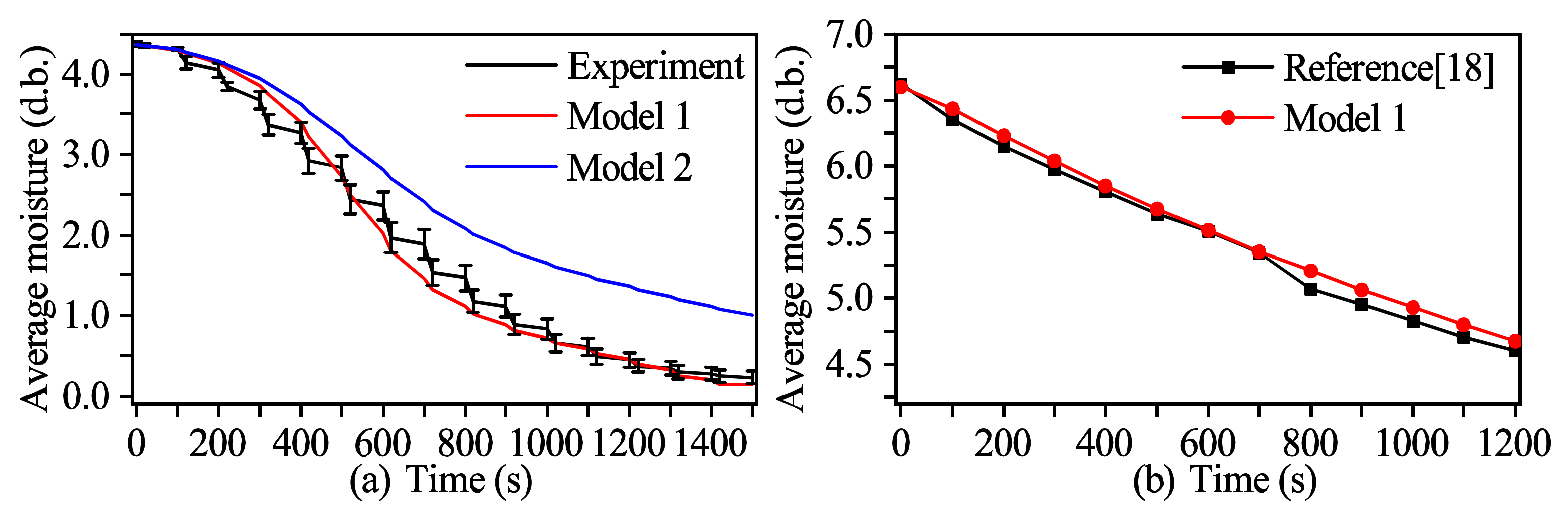
3.1.1. Moisture Content

As shown in Figure 4a, the results of the average moisture content on dry basis obtained by the models with and without considering deformation were compared with the experimental data. The error bars on the curve of the experimental data represented the values of the measurement uncertainty. Additionally, in order to express the theoretical models with and without considering deformation concisely, we named the model considering deformation as Model 1 and the model not considering deformation as Model 2.

The average moisture content obtained by Model 1 decreased from 4.374 to 0.137, being located within the range consisting of the measuring values and the measurement uncertainty. It matched better with the experimental data with a higher coefficient of determination of ${\mathrm{R}}^2=0.987$ and a lower root mean square error of $\mathrm{RMSE}=0.180$. The results of the average moisture content obtained by Model 2 decreased from 4.374 to 1.001, which was higher than the experimental data with a lower coefficient of determination of ${\mathrm{R}}^2=0.739$ and a higher root mean square error of $\mathrm{RMSE}=0.678$. This was because during the thermal process, the deformation caused an additional flow of the fluid phases. Thus, the results of Model 1 were more consistent with the experimental data, namely, it was more in line with the actual situation. A similar conclusion has also been drawn by Gulati et al. [43].

In order to improve the reliability of the model developed in this study, we applied Model 1 to simulate the intermittent microwave convective drying of apple slice studied in [18]. The average moisture content obtained by Model 1 was compared with the experimental results obtained in [18], as shown in Figure 4b. A good consistence of the two results can be observed. Thus, it indicates that the model developed in our study could be extended to the application of other microwave thermal processes and could gain accurate simulation results.

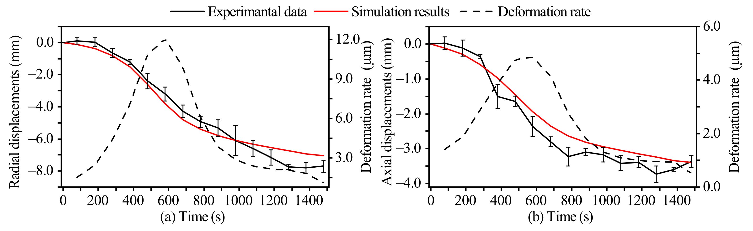
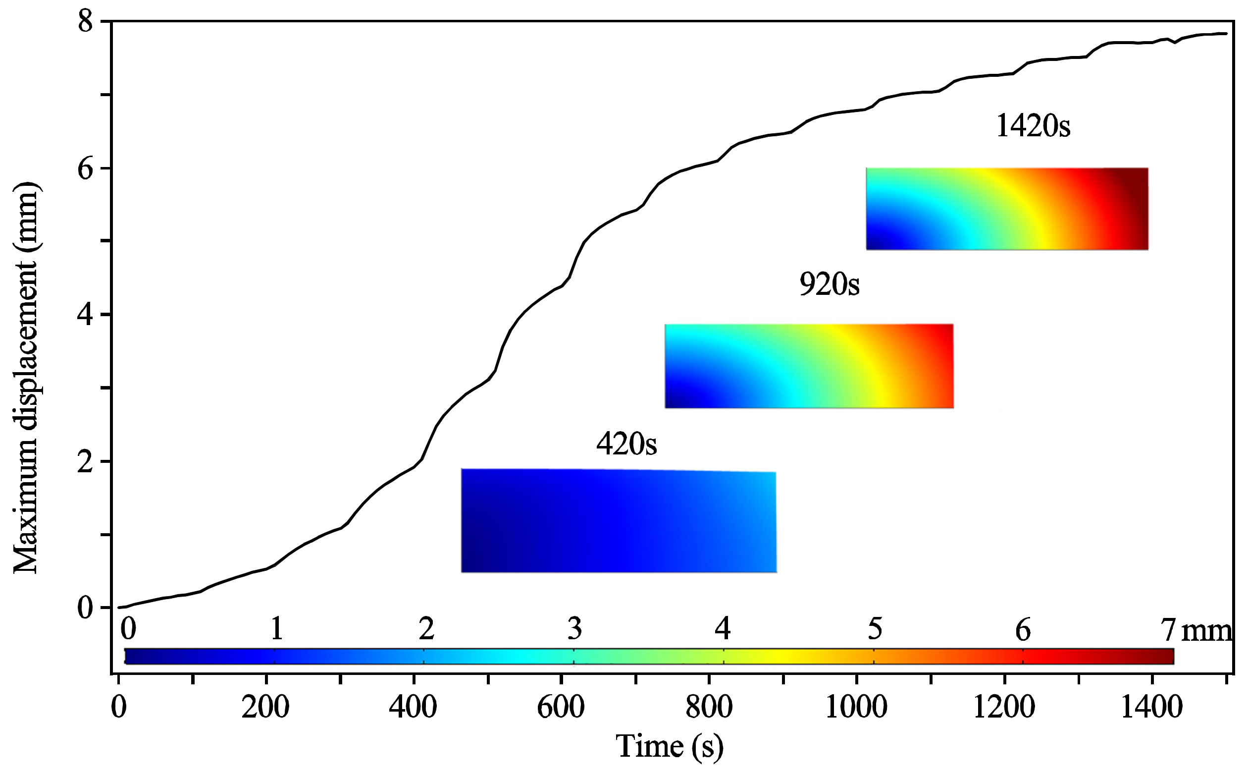
3.1.2. Deformation Displacements

As shown in Figure 5a,b, the simulation results of the radial and axial displacements are presented and compared with the experimental data. The error bars on the curves of the experimental data represent the values of the measurement uncertainty. The negative values indicated the shrinkage of the sample. The radial and axial displacements obtained by Model 1 were −7.04 mm and −3.39 mm, respectively; the values of the coefficient of determination of the radial and axial displacements ${\mathrm{R}}^2=0.963$ and ${\mathrm{R}}^2=0.926$, respectively; and the values of the root mean square error of the radial and axial displacements were $\mathrm{RMSE}=0.506\hspace{0.33em}\mathrm{mm}$ and $\mathrm{RMSE}=0.335\hspace{0.33em}\mathrm{mm}$, respectively. Most of the simulation results were located within the range consisting of the measuring values and the measurement uncertainty. Therefore, the simulation results of the radial and axial displacements matched well with the experimental data. Moreover, the deformation rates are also given in Figure 5, which indicates that the deformation rate reached the global maximum around 600 s due to the collapse of cell structure caused by moisture loss [56].

3.1.3. Temperature

In Figure 6, the temperature results at the top surface center of the sample obtained by Model 1 and Model 2 are compared with the experimental data, and the error bars on the curves of the experimental data represent the values of the measurement uncertainty. The temperature obtained by the experiment ranged from $29.9 °\mathrm{C}$ to $73.65 °\mathrm{C}$, and the values of the temperature obtained by Model 1 and Model 2 ranged from $30.0 °\mathrm{C}$ to $86.17 °\mathrm{C}$ and ranged from $30.0 °\mathrm{C}$ to $85.34 °\mathrm{C}$, respectively. Most of the simulation results were located out of the range consisting of the measuring values and the measurement uncertainty. Moreover, the coefficients of determination and the root mean square errors of the two models were ${\mathrm{R}}^2=0.437$ and ${\mathrm{R}}^2=0.345$, and $\mathrm{RMSE}=13.5 °\mathrm{C}$ and $\mathrm{RMSE}=15.4 °\mathrm{C}$, respectively. This indicates that the simulated temperature values were higher than the experimental data. However, there was temperature deviation between the simulation results and the experimental data, and the temperature trends of both models were similar to the experimental data. Thus, the models can be used to describe the temperature tendency.

There were two reasons for this large temperature deviation between the simulation and experimental results. One was the inevitable measuring error of the hand-held infrared thermometer; the other reason was the usage of Lambert’s law to calculate the electric filed. Lambert’s law is based on the semi-infinite critical sample length assumption, and it does not consider the standing wave effects [57]. Moreover, the power absorption on the surface is always the maximum, regardless of the moisture content [18,58]. Similar overestimations of the temperature obtained by the models using Lambert’s law have also been observed in previous studies, and the Maxwell’s equations are more ideal in modelling the microwave heat generation and the standing wave effects [18,57]. Therefore, we used the Maxwell’s equations to simulate the distribution of the electromagnetic field within the sample in our next stage of study.

3.2. Discussions about the Mechanisms of Different Phenomena

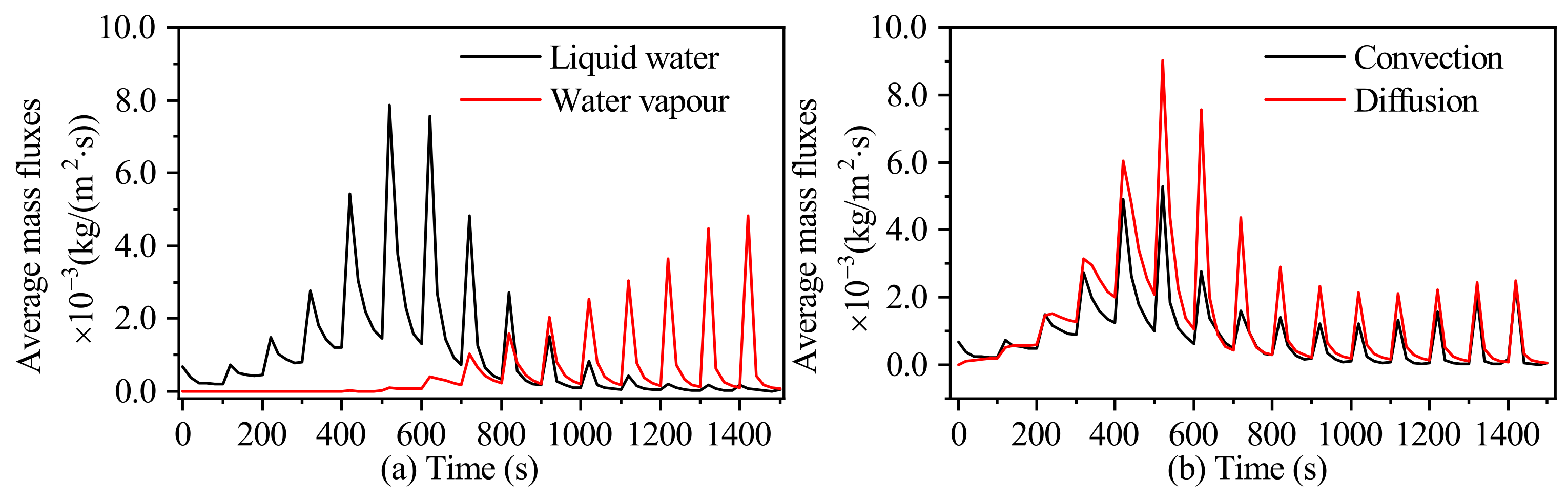
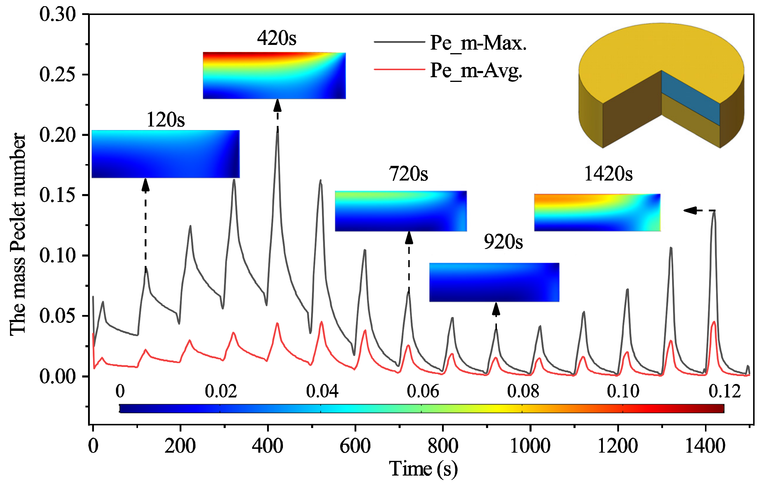
3.2.1. The Mass Transport Mechanism

The curves in Figure 7a,b present the time evolution of the average values of the mass fluxes of different fluid phases and those under different driving forces, respectively. As shown in Figure 7a, initially, the average flux of liquid water was higher than that of water vapor by three orders of magnitude on average; then, the average flux of liquid water turned to being lower than that of water vapor by one order of magnitude on average. Thus, combining the time evolution curves of the moisture content, as shown in Figure 4a, the removing of liquid water was first the main part of the entire moisture removing, which made the moisture content decrease from 4.37 to 1.11; then, the removing of water vapor turned to being predominant, which made the moisture content decrease from 1.11 to 0.14. This is consistent with the statements in [16,17]. Therefore, during the IMW thermal process, when the moisture content was high, the moisture loss was caused by the removal of the liquid water first; then, it turned to water vapor when the moisture content was low.

As shown in Figure 7b, the values of the diffusion flux driven by concentration gradients and those of the convective flux driven by pressure gradients were on the same order of magnitude, and the values of the former were slightly higher. Thus, the diffusion flux contributed more to the moisture loss. In addition, the Peclet number (Pe) defined as the ratio of the convective (mass/heat) transport to the diffusion (mass/heat) transport [59,60] was used to reflect the dominant mechanism of the (mass/heat) transport. In Figure 8, the time evolution curves of the maximum and average mass Pe and the distribution diagrams of the mass Pe at some specific time points are presented. In each cycle, the mass Pe increased to a peak value after the heating stage, then decreased to a valley value after the tempering stage. The peak values of the maximum mass Pe ranged from 0.04 to 0.20, and those of the average mass Pe ranged from 0.01 to 0.05. All the peak values were less than 1.00. Namely, the mass transport by diffusion driven by the concentration gradient was larger than that by convection driven by the gas pressure gradient. Thus, the diffusion was the dominant mechanism of the mass transport during the whole IMW thermal process, which is consistent with the conclusion drawn from Figure 7b. From the mass Pe distribution diagrams shown in Figure 8, the mass Pe was relatively large near the surface due to the higher velocity of the liquid phase.

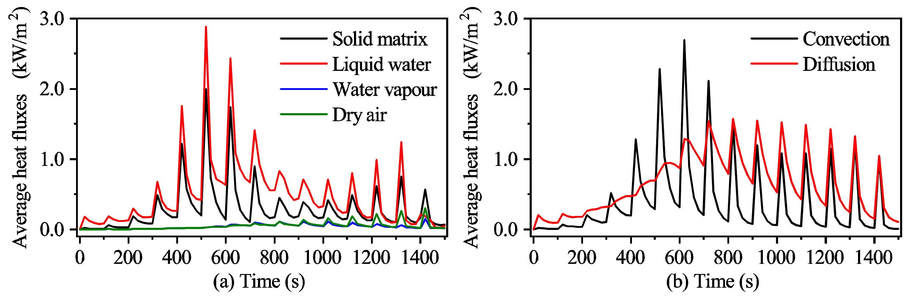
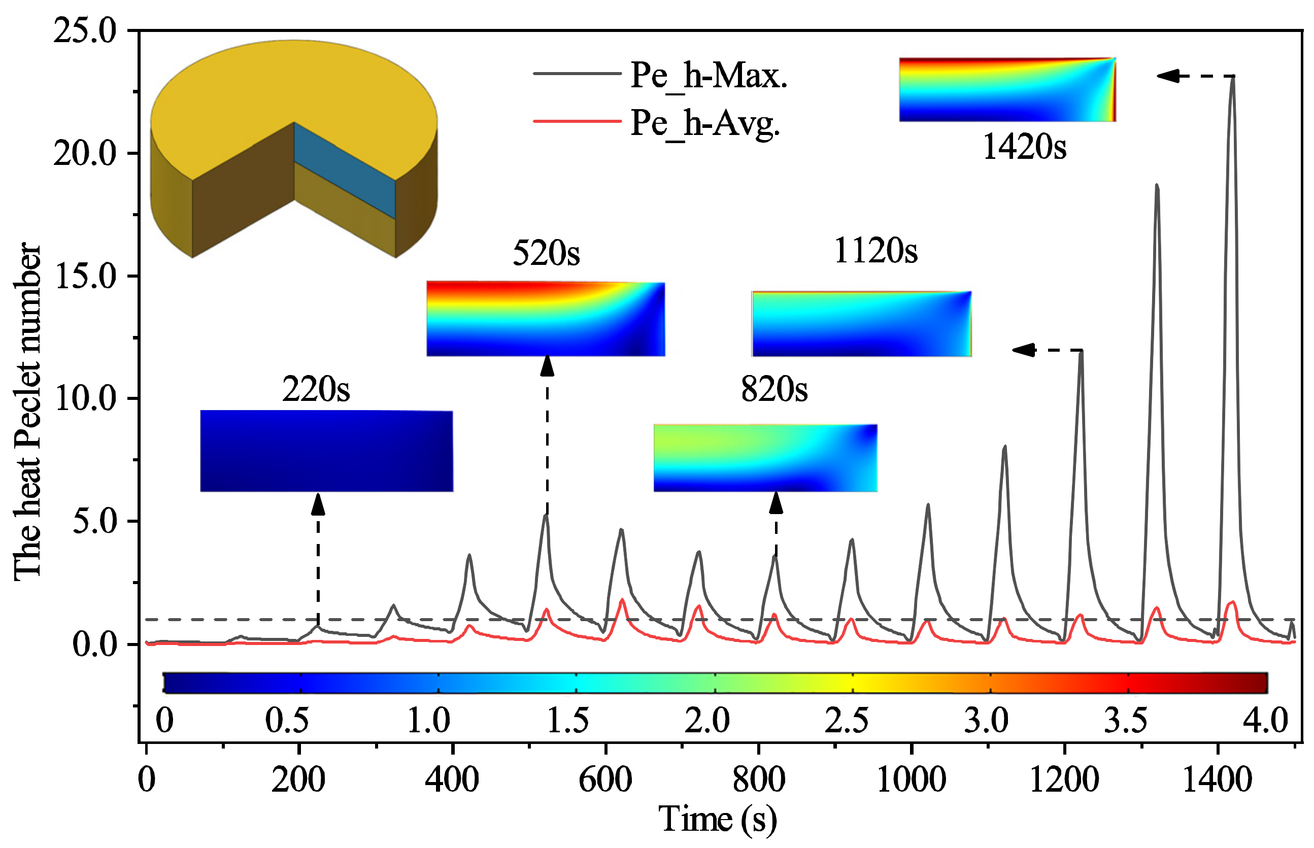
3.2.2. The Heat Transport Mechanism

The curves in Figure 9a,b demonstrate the average heat fluxes of different phases and different heat transfer methods, respectively. In Figure 9a, the heat fluxes of liquid water and solid phase were on the same order of magnitude, and both were higher than those of water vapor and dry air by one order of magnitude. Thus, the liquid water and the solid phase were the principal media carrying heat. From Figure 9b, we see that both convective and diffusion heat fluxes were on the same order of magnitude, and the two values were comparable. Except for the period between $300\hspace{0.33em}\mathrm{s}$ and $700\hspace{0.33em}\mathrm{s}$, the peak values of the average diffusion heat flux were higher than those of the average convection heat flux. The valley values of the average diffusion heat flux were always higher than those of the average convection heat flux during the whole process.

In Figure 10, the time evolution curves of the maximum and average heat Pe and the distribution diagrams of the heat Pe at some specific time points are presented. In each cycle, the heat Pe increased to a peak value after the heating stage, then decreased to a valley value after the tempering stage. The peak values of the maximum heat Pe ranged from $0.14$ to $23.15$, and those of the average heat Pe ranged from $0.03$ to $1.73$. Most of the peak values of the maximum and average heat Pe were larger than $1.00$, and all of the valley values were lower than $1.00$. Namely, the convective heat flux was the dominant mechanism in most of the heating stage, and then the diffusion heat flux turned to being dominant in the tempering stage of all cycles.

Furthermore, as shown in Figure 8 and Figure 10, the peak values of both mass and heat Pe reached local maxima in the middle and final stages of the whole processes, respectively. In the middle stage, the increase in the peak values of Pe resulted from the increase in the velocities of liquid water and solid deformation. On the other hand, in the final stage, the increase in the peak values of Pe was caused by the increase in the velocity of water vapor.

3.2.3. The von Mises Stress

The von Mises stress, based on the fourth strength theory, is used to predict the quality attribute of the sample (e.g., the failure or crack of the material). The time evolution curves of the maximum and average von Mises stress are shown in Figure 11. Moreover, the von Mises stress distribution diagrams at some specific time points are presented in Figure 11.

In each cycle, the von Mises stress increased to a peak value after the heating stage, then decreased to a valley value after the tempering stage. The peak values of the maximum von Mises stress ranged from $0.01\hspace{0.33em}\mathrm{MPa}$ to $0.36\hspace{0.33em}\mathrm{MPa}$, and those of the average von Mises stress ranged from $0.00\hspace{0.33em}\mathrm{MPa}$ to $0.15\hspace{0.33em}\mathrm{MPa}$. It revealed that the curves of the maximum and average von Mises stresses shared a similar trend. Namely, the peak values of both stresses reached the local maxima of $0.18\hspace{0.33em}\mathrm{MPa}$ and $0.05\hspace{0.33em}\mathrm{MPa}$ at $520\hspace{0.33em}\mathrm{s}$, respectively; then, the peak values of both stresses reached another local maxima of $0.36\hspace{0.33em}\mathrm{MPa}$ and $0.15\hspace{0.33em}\mathrm{MPa}$ at $1420\hspace{0.33em}\mathrm{s}$, respectively. In addition, the local maximum stress at $520\hspace{0.33em}\mathrm{s}$ appeared on the sample surface, while that at $1420\hspace{0.33em}\mathrm{s}$ was in the material. The reason for the first local maximum stress was the high gradients of temperature, gas pressure, water vapor concentration, and liquid water concentration [43]. On the other hand, the second local maximum stress was due to the glass transition of the material, which made the elastic modulus larger and the Poisson’s ratio lower. Moreover, material failure or crack would appear at a location if the stress there was above the fracture stress. Thus, the crack or fracture most likely occurred at the locations with the local maximum stress. Therefore, the fracture most likely appeared on the sample surface at $520\hspace{0.33em}\mathrm{s}$ or inside the materials at $1420\hspace{0.33em}\mathrm{s}$. On the other hand, the fracture stress of potato was on the order of $1\times {10}^6\hspace{0.33em}\mathrm{Pa}$ magnitude [43,52], which was higher than the maxima von Mises stress in the sample shown in Figure 11. Therefore, in the sample of our study, crack or fracture of the product can be avoided, and drying product can be obtained in a good quality. This was validated by the final state of the potato sample shown in Figure 2e.

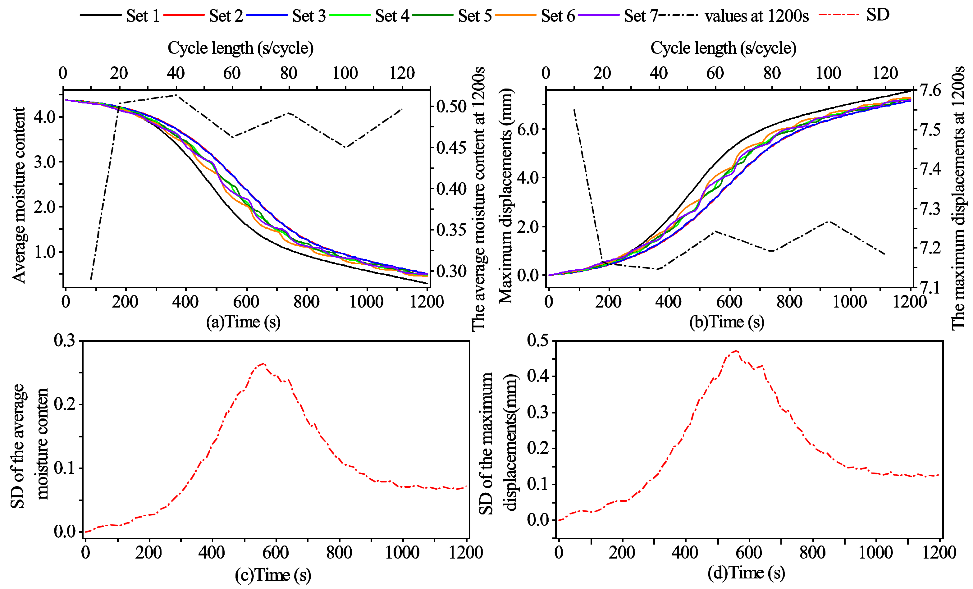
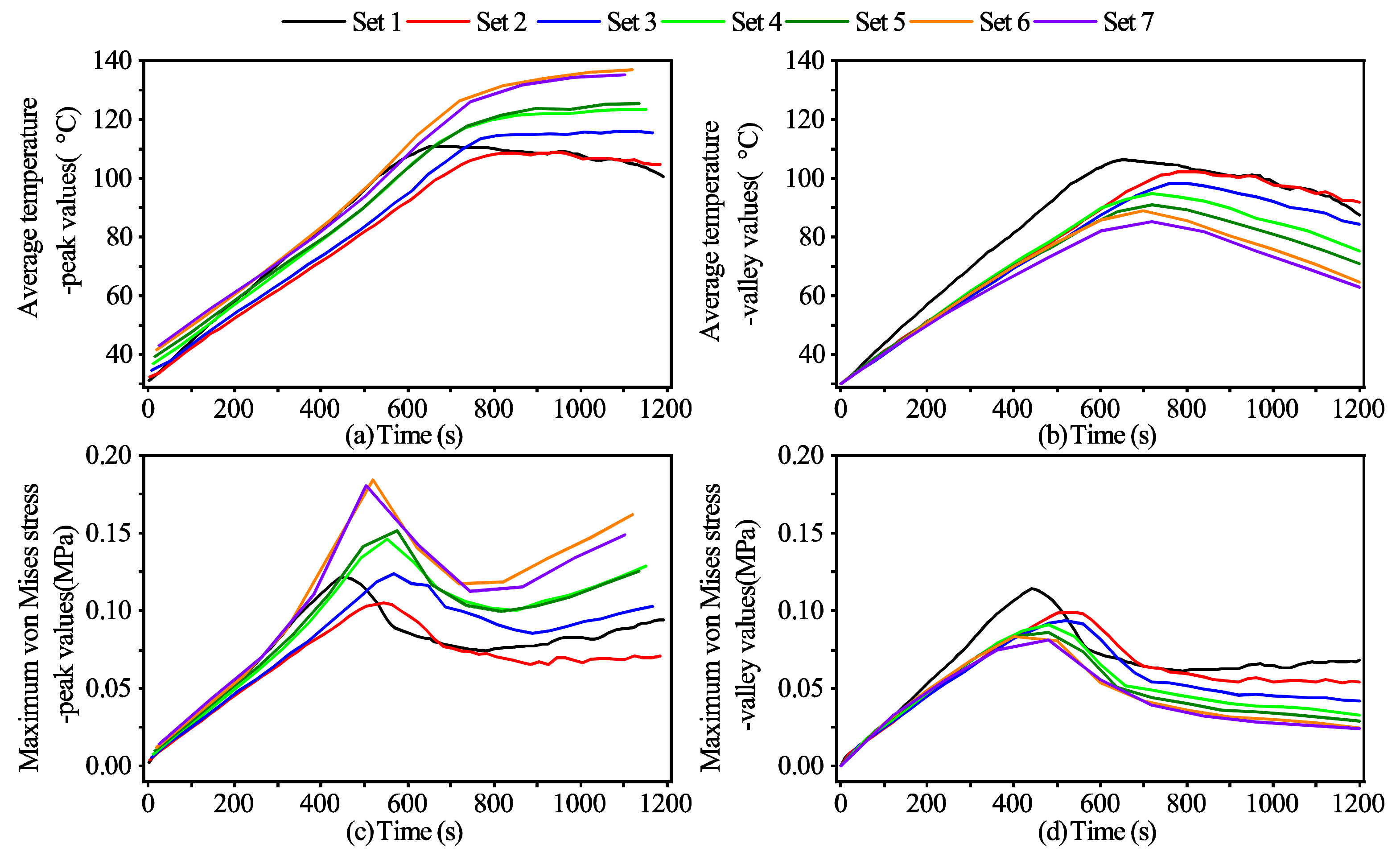
3.3. The Effects of the Cycle Length on the Outcomes

The power ratio or pulse ratio (PR) is a critical parameter used in the intermittent process. It is defined as the ratio of the total time length of a cycle to the heating time in the cycle or its inverse [61,62,63]. From previous studies, it was revealed that prolonging the tempering time is of benefit to the quality improvement of the products [61,62,63]. However, there is no study on the effects of the cycle length on the results of the process with the same PR. Thus, in this section, we focus on the effects of the cycle length on the results of the porous dielectric material in the IMW thermal process. The settings of different cycle lengths are shown in

Table 2. The samples with different cycle lengths.

	Set 1	Set 2	Set 3	Set 4	Set 5	Set 6	Set 7
Cycle length	10 s/cycle	20 s/cycle	40 s/cycle	60 s/cycle	80 s/cycle	100 s/cycle	120 s/cycle
Heating, s	2	4	8	12	16	20	24
Tempering, s	8	16	32	48	64	80	96
PR	5	5	5	5	5	5	5
Cycles	120	60	30	20	15	12	10

.

In Figure 12a,b, the solid lines are the time evolution curves of the average moisture content on dry basis and the maximum displacement, respectively; the dot-dashed lines are the values of the average moisture content and the maximum displacement of different settings at 1200 s. From Figure 12a,b, it can be seen that the fluctuations of the time evolution curves increased with the prolonging of the cycle length. The changing rate of the longer cycle length was also higher.

The average moisture of Set 1 was the lowest, changing from $4.37$ to $0.29$, and that of Set 3 was the highest, changing from $4.37$ to $0.51$. Similarly, the maximum displacement of Set 1 was the highest, with a changing range from 0.00 mm to 7.55 mm, and that of Set 3 was the lowest, changing from 0.00 mm to 7.15 mm. At 1200 s, the final values of the average moisture content and the maximum displacement of different settings presented fluctuations with the cycle length. Namely, the final average moisture content of Set 1 was the lowest at $0.29$, and that of Set 3 was the highest at $0.51$. The final maximum displacement of Set 1 was the highest at 7.55 mm, and that of Set 3 was the lowest at 7.15 mm. In addition, we used the standard deviation (SD) to evaluate the gap among different simulation results, as shown in Figure 12c,d. It indicated that the gap among different settings reached the global maximum between 500 s and 600 s, which resulted from the high water loss and deformation rates at this stage.

In Figure 13a,b, the time evolution curves of the peak and valley values of the average temperature are presented, and those of the maximum von Mises stress are presented in Figure 13c,d. From Figure 13a, the peak values of the average temperature of different settings shared a similar trend, which increased firstly and then kept stable. As a whole, the peak values of the average temperature of different settings increased with the cycle length. Similarly, the valley values of the average temperature of different settings decreased with the cycle length, as shown in Figure 13b. In Figure 13c,d, the peak and valley values of the maximum von Mises stress also increased and decreased with the cycle length as a whole, respectively. In addition, both the peak and valley values of the von Mises stress both reached local maximum values around 500 s, which resulted from the high gradients of the moisture content, temperature, deformation, and pressure at this stage [43].

Therefore, from the above comparisons of the results of different cycle lengths, we found that the fluctuations of the outcomes became larger with the increase of the cycle length.

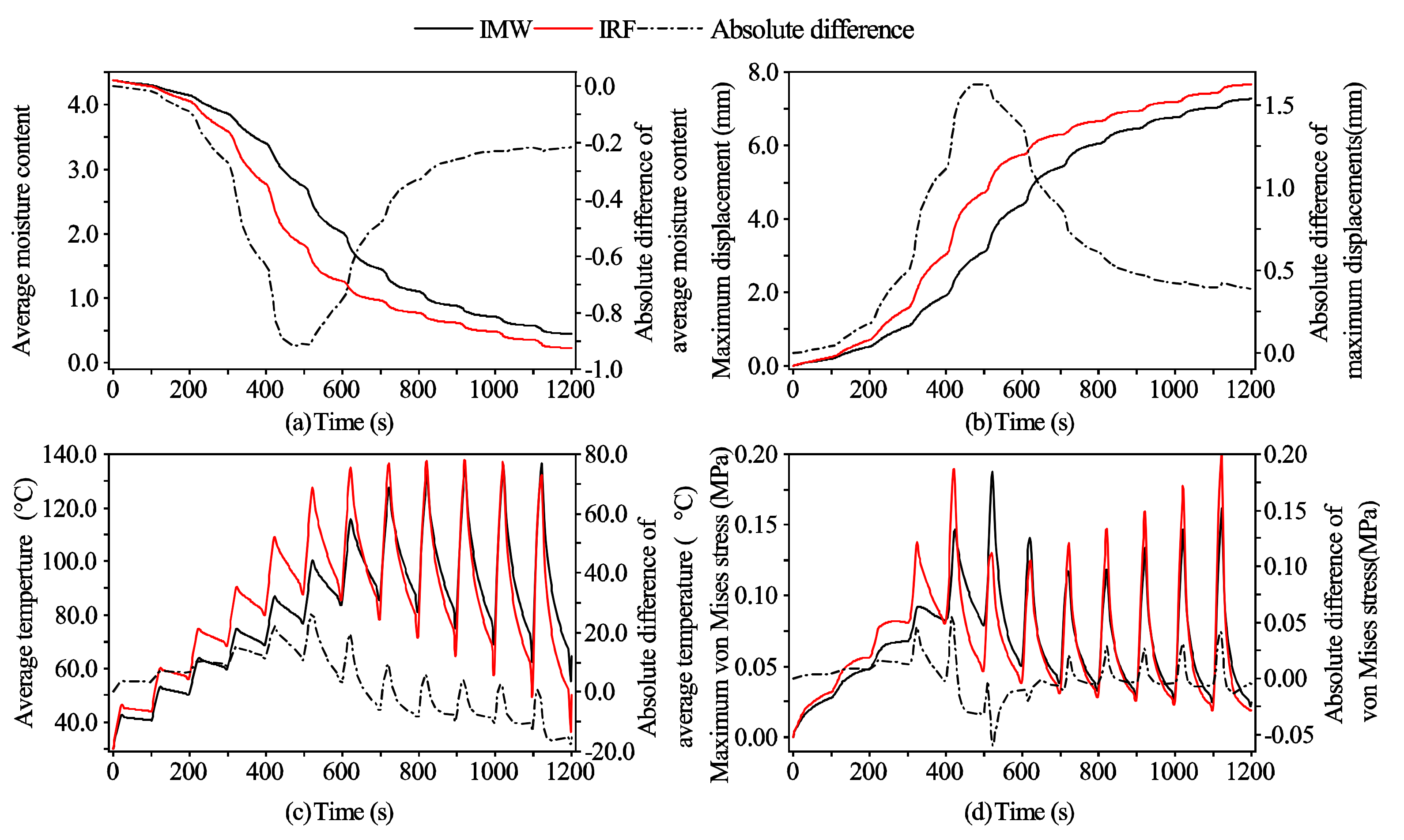
3.4. The Effects of the Frequency on the Outcomes

The differences between the radio frequency (RF) and the microwave thermal processes were all caused by their frequency difference [8]. The model developed in our study can be extended to simulate the IRF thermal process. We compare the results of the IMW and the IRF thermal processes in this section. The time evolution curves of the average moisture content, the maximum displacement, the average temperature, and the maximum von Mises stress are presented in Figure 14a–d, respectively. Moreover, the absolute differences between the results of the IMW and IRF (i.e., the values obtained by the IRF minus those obtained by the IMW) are also presented in these figures.

As shown in Figure 14a, the average moisture content of the IRF was lower than that of the IMW. Namely, the average moisture content of the IRF decreased from $4.37$ to $0.23$, and that of the IMW decreased from $4.37$ to $0.45$. In Figure 14b, the maximum displacement of the IRF was higher than that of the IMW. Namely, the maximum displacement of the IRF increased from 0.00 mm to 7.66 mm, and that of the IMW increased from 0.00 mm to 7.27 mm. Therefore, if the dielectric materials need to be dried with a higher efficiency, the IRF is a better choice, while if the purpose of the thermal process is heating with less water loss and deformation, then the IMW is more ideal instead. In addition, both of the absolute differences of the average moisture content and the maximum displacement of the two processes had global extremes around 500 s, being $-0.91$ and 1.63 mm, respectively. This was due to the violent transport of mass and heat at this period of time.

As shown in Figure 14c,d, in the heating stage of each cycle, the average temperature and the maximum stress of the material treated by the IRF increased faster than those treated by the IMW. In the tempering stage of each cycle, the average temperature and the maximum stress of the material treated by the IRF decreased faster than those treated by the IMW. In Figure 14c, the average temperature peak values of the IRF were higher than those of the IMW. While the average temperature valley values of the IRF were higher than those of the IMW before 600 s, they then turned to be lower thereafter. The absolute differences of the average temperature between the two processes reached a global maximum of 27.22 °C at 520 s. Therefore, the temperature of the material treated by the IRF increased faster than that treated by the IMW; however, the average temperature peak values of the materials treated by both processes tended to reach a similar equilibrium and stayed constant thereafter. In Figure 14d, the peak values of the maximum stress of the IRF was higher than those of the IMW, except for the period between 420 s and 700 s, while the valley values of the IRF were higher before 400 s, and then the values were lower than those of the IMW thereafter. The maximum stress peak values of both processes reached local maxima in the middle stage and then decreased to the local minima, and the local maximum of the IRF reached earlier than that of the IMW. Namely, the stress peak values of the material treated by the IRF reached a local maximum of $0.19\hspace{0.33em}\mathrm{MPa}$ at $420\hspace{0.33em}\mathrm{s}$, then decreased to a local minimum of $0.12\hspace{0.33em}\mathrm{MPa}$ at $620\hspace{0.33em}\mathrm{s}$, and those of the material treated by the IMW reached a local maximum of $0.18\hspace{0.33em}\mathrm{MPa}$ at $520\hspace{0.33em}\mathrm{s}$, then decreased to a local minimum of $0.12\hspace{0.33em}\mathrm{MPa}$ at $720\hspace{0.33em}\mathrm{s}$. The stress valley values of both processes reached a global maximum of $0.08\hspace{0.33em}\mathrm{MPa}$ at $400\hspace{0.33em}\mathrm{s}$. Therefore, the maximum stress in the material treated by the IRF was similar to that treated by the IMW in the aspect of amplitudes and trends, both were lower than the fracture stress. The difference between the two processes was that the local maximum of the IRF arrived earlier than that of the IMW, which was due to the deeper electromagnetic energy penetration of the IRF.

4. Conclusions

A 2D axi-symmetric physically based theoretical model was developed, and the electromagnetic energy, multiphase transport, phase change, large deformation, and glass transition were taken into consideration. The model was validated by an IMW experiment, as well as the experimental results of other researchers. Therefore, the model can be used in various processes (e.g., microwave thermal processes, radio frequency thermal processes, and even other thermal processes) of different porous media. When the model is employed in a specific industrial application, only the physical parameters of the corresponding materials and the environment need to be set. It can uncover the mechanisms of the mass and heat transport intuitively and can be used to optimize the process parameters in an efficient and economical way on the basis of the simulation results of temperature, moisture content, and deformation.

From our simulation results and discussions, it can be concluded that the mass was mainly carried by liquid water when the moisture content was high, and turned to being carried by water vapor when the moisture content became low. The heat was mainly carried by liquid water and solid. By comparing the average fluxes and Pe numbers of the mass and heat, we found that the diffusion was the dominant mechanism of the mass transport during the whole process. For the heat transport, the diffusion was the dominant mechanism during the tempering stage, while the convection dominated the heat transport near the surface areas of the material during the heating stage. In our study, throughout the whole process, the von Mises stress was lower than the fracture stress. The von Mises stress reached a local maximum on the top surface of material in the middle stage due to the high gradients of the moisture content, deformation, and temperature, and it reached another local maximum inside the material at the final stage due to the glass transition of the material.

For the intermittent thermal process, different cycle lengths with the same PR affected the outcomes. In our study, the setting of 10 s/cycle led to the outcomes with the lowest moisture content and the largest deformation, the setting of 30 s/cycle led to the outcomes with the highest moisture content and the least deformation, and the outcomes of other settings lay between them. Moreover, the fluctuations of the outcomes of the moisture content, deformation, temperature, and von Mises stress became larger with the increasing of the cycle length. Thus, the material treated by a longer cycle length tended to trigger the phenomena of overheat and fracture.

The model in our study can be used to simulate both the IMW and IRF thermal processes. By comparing the results of the two thermal processes, we found that the IRF process tended to obtain the lower moisture content and the larger deformation. Moreover, the outcomes of the temperature and von Mises stress in the two processes were similar. The only difference was that the IRF reached the local maxima earlier than the IMW due to the deeper penetration of the electromagnetic energy. Thus, for the drying process, the IRF was found to be more suitable due to its lower moisture content outcome, while for the heating process requiring less deformation, the IMW can be said to be more ideal.

References

1. Schubert, H.; Regier, M. The Microwave Processing of Foods; CRC Press LLC: Boca Raton, FL, USA; Woodhead Publisher Limited: Cambridge, UK, 2005. [Google Scholar]
2. Zhao, P.; Liu, C.; Qu, W.; He, Z.; Gao, J.; Jia, L.; Ji, S.; Ruan, R. Effect of Temperature and Microwave Power Levels on Microwave Drying Kinetics of Zhaotong Lignite. Processes 2019, 7, 74. [Google Scholar] [CrossRef] [Green Version]
3. Wang, H.; Liu, D.; Yu, H.; Wang, D.; Li, J. Optimization of Microwave Coupled Hot Air Drying for Chinese Yam Using Response Surface Methodology. Processes 2019, 7, 745. [Google Scholar] [CrossRef] [Green Version]
4. Soni, A.; Smith, J.; Thompson, A.; Brightwell, G. Microwave-induced thermal sterilization—A review on history, technical progress, advantages and challenges as compared to the conventional methods. Trends Food Sci. Technol. 2020, 97, 433–442. [Google Scholar] [CrossRef]
5. Huang, Z.; Chen, L.; Wang, S. Computer simulation of radio frequency selective heating of insects in soybeans. Int. J. Heat Mass Transf. 2015, 90, 406–417. [Google Scholar] [CrossRef]
6. Kumar, C.; Karim, M.A.; Joardder, M.U.H. Intermittent drying of food products: A critical review. J. Food Eng. 2014, 121, 48–57. [Google Scholar] [CrossRef] [Green Version]
7. Rosa, A.R.D.; Bressan, F.; Leone, F.; Falqui, L.; Chiofalo, V. Radio frequency heating on food of animal origin: A review. Eur. Food Res. Technol. 2019, 245, 1787–1797. [Google Scholar] [CrossRef]
8. Ramaswamy, H.S. Radio-Frequency Heating in Food Processing Principles and Applications; CRC Press: Boca Raton, FL, USA, 2014; p. 422. [Google Scholar]
9. Thuto, W.; Banjong, K. Investigation of Heat and Moisture Transport in Bananas during Microwave Heating Process. Processes 2019, 7, 545. [Google Scholar] [CrossRef] [Green Version]
10. Hou, L.; Zhou, X.; Wang, S. Numerical analysis of heat and mass transfer in kiwifruit slices during combined radio frequency and vacuum drying. Int. J. Heat Mass Transf. 2020, 154, 119704. [Google Scholar] [CrossRef]
11. Fu, B.A.; Chen, M.Q. Linear non-equilibrium thermal and deformation transport model for hematite pellet in dielectric and magnetic heating. Appl. Therm. Eng. 2020, 173, 115197. [Google Scholar] [CrossRef]
12. Li, H.; Shi, S.; Lin, B.; Lu, J.; Lu, Y.; Ye, Q.; Wang, Z.; Hong, Y.; Zhu, X. A fully coupled electromagnetic, heat transfer and multiphase porous media model for microwave heating of coal. Fuel Process. Technol. 2019, 189, 49–61. [Google Scholar] [CrossRef]
13. Itaya, Y.; Uchiyama, S.; Mori, S. Internal Heating Effect and Enhancement of Drying of Ceramics by Microwave Heating with Dynamic Control. Transp. Porous Media 2006, 66, 29–42. [Google Scholar] [CrossRef]
14. Jalili, M.; Anca-Couce, A.; Zobel, N. On the Uncertainty of a Mathematical Model for Drying of a Wood Particle. Energy Fuels 2013, 27, 6705–6717. [Google Scholar] [CrossRef]
15. Rattanadecho, P.; Keangin, P. Numerical study of heat transfer and blood flow in two-layered porous liver tissue during microwave ablation process using single and double slot antenna. Int. J. Heat Mass Transf. 2013, 58, 457–470. [Google Scholar] [CrossRef]
16. Datta, A.K. Porous media approaches to studying simultaneous heat and mass transfer in food processes. I: Problem formulations. J. Food Eng. 2007, 80, 80–95. [Google Scholar] [CrossRef]
17. Datta, A.K. Porous media approaches to studying simultaneous heat and mass transfer in food processes. II: Property data and representative results. J. Food Eng. 2007, 80, 96–110. [Google Scholar] [CrossRef]
18. Kumar, C.; Joardder, M.U.H.; Farrell, T.W.; Karim, M.A. Multiphase porous media model for intermittent microwave convective drying (IMCD) of food. Int. J. Therm. Sci. 2016, 104, 304–314. [Google Scholar] [CrossRef]
19. Mahiuddin, M.; Khan, M.I.H.; Kumar, C.; Rahman, M.M.; Karim, M.A. Shrinkage of Food Materials during Drying: Current Status and Challenges. Compr. Rev. Food Sci. Food Saf. 2018, 17, 1113–1126. [Google Scholar] [CrossRef] [Green Version]
20. Datta, A.K. Toward computer-aided food engineering: Mechanistic frameworks for evolution of product, quality and safety during processing. J. Food Eng. 2016, 176, 9–27. [Google Scholar] [CrossRef]
21. Pabis, S. Theoretical models of vegetable drying by convection. Transp. Porous Media 2007, 66, 77–87. [Google Scholar] [CrossRef]
22. Onwude, D.I.; Hashim, N.; Abdan, K.; Janius, R.; Chen, G. Numerical modeling of radiative heat and mass transfer for sweet potato during drying. J. Food Process. Preserv. 2018, 42, e13741. [Google Scholar] [CrossRef]
23. Onwude, D.I.; Hashim, N.; Abdan, K.; Janius, R.; Chen, G. Experimental studies and mathematical simulation of intermittent infrared and convective drying of sweet potato (Ipomoea batatas L.). Food Bioprod. Process. 2019, 114, 163–174. [Google Scholar] [CrossRef]
24. Joardder, M.U.H.; Karim, M.A. Development of a porosity prediction model based on shrinkage velocity and glass transition temperature. Dry. Technol. 2019, 37, 1988–2004. [Google Scholar] [CrossRef] [Green Version]
25. Joardder, M.U.H.; Kumar, C.; Karim, M.A. Multiphase transfer model for intermittent microwave-convective drying of food: Considering shrinkage and pore evolution. Int. J. Multiph. Flow 2017, 95, 101–119. [Google Scholar] [CrossRef]
26. Rakesh, V.; Datta, A. Microwave puffing: Mathematical modeling and optimization. In Proceedings of the 11th International Congress on Engineering and Food (ICEF), Athens, Greece, 22–26 May 2011; pp. 762–769. [Google Scholar]
27. Rakesh, V.; Datta, A.K. Microwave puffing: Determination of optimal conditions using a coupled multiphase porous media-Large deformation model. J. Food Eng. 2011, 107, 152–163. [Google Scholar] [CrossRef]
28. Rakesh, V.; Datta, A.K. Transport in Deformable Hygroscopic Porous Media during Microwave Puffing. AIChE J. 2012, 59, 33–45. [Google Scholar] [CrossRef]
29. Zhang, J.; Datta, A.K.; Mukherjee, S. Transport Processes and Large Deformation During Baking of Bread. AIChE J. 2005, 51, 2569–2580. [Google Scholar] [CrossRef]
30. Niamnuy, C.; Devahastin, S.; Soponronnarit, S.; Raghavan, G.S.V. Modeling coupled transport phenomena and mechanical deformation of shrimp during drying in a jet spouted bed dryer. Chem. Eng. Sci. 2008, 63, 5503–5512. [Google Scholar] [CrossRef]
31. Timoumi, S.; Mihoubi, D.; Zagrouba, F. Modelling of Moisture Content, β-Carotene and Deformation Variation during Drying of Carrot. Int. J. Food Eng. 2019, 15, 20180155. [Google Scholar] [CrossRef]
32. Curcio, S.; Aversa, M. Influence of shrinkage on convective drying of fresh vegetables: A theoretical model. J. Food Eng. 2014, 123, 36–49. [Google Scholar] [CrossRef]
33. Yang, H.; Sakai, N.; Watanabe, M. Drying model with non-isotropic shrinkage deformation undergoing simultaneous heat and mass transfer. Dry. Technol. 2001, 19, 1441–1460. [Google Scholar] [CrossRef]
34. Aregawi, W.A.; Defraeye, T.; Verboven, P.; Herremans, E.; Roeck, G.D.; Nicolai, B.M. Modeling of Coupled Water Transport and Large Deformation During Dehydration of Apple Tissue. Food Bioprocess Technol. 2013, 6, 1963–1978. [Google Scholar] [CrossRef] [Green Version]
35. Li, X.; Llave, Y.; Mao, W.; Fukuoka, M.; Sakai, N. Heat and mass transfer, shrinkage, and thermal protein denaturation of kuruma prawn (Marsupenaeus japonicas) during water bath treatment: A computational study with experimental validation. J. Food Eng. 2018, 238, 30–43. [Google Scholar] [CrossRef]
36. Llave, Y.; Takemori, K.; Fukuoka, M.; Takemori, T.; Tomita, H.; Sakai, N. Mathematical modeling of shrinkage deformation in eggplant undergoing simultaneous heat and mass transfer during convection-oven roasting. J. Food Eng. 2016, 178, 124–136. [Google Scholar] [CrossRef]
37. Kowalski, S.J.; Smoczkiewicz-Wojciechowska, A. Stresses in dried wood. Modelling and experimental identification. Transp. Porous Media 2006, 66, 145–158. [Google Scholar] [CrossRef]
38. Heydari, M.; Khalili, K. Investigation on the Effect of Young’s Modulus Variation on Drying-Induced Stresses. Transp. Porous Media 2016, 112, 519–540. [Google Scholar] [CrossRef]
39. Mihoubi, D.; Bellagi, A. Stress Generated During Drying of Saturated Porous Media. Transp. Porous Media 2009, 80, 519–536. [Google Scholar] [CrossRef]
40. Kowalski, S.J.; Rybicki, A. Drying stress formation by inhomogeneous moisture and temperature distribution. Transp. Porous Media 1996, 24, 139–156. [Google Scholar] [CrossRef]
41. Defraeye, T.; Radu, A. Insights in convective drying of fruit by coupled modeling of fruit drying, deformation, quality evolution and convective exchange with the airflow. Appl. Therm. Eng. 2018, 129, 1026–1038. [Google Scholar] [CrossRef]
42. Gulati, T.; Datta, A.K. Mechanistic understanding of case-hardening and texture development during drying of food materials. J. Food Eng. 2015, 166, 119–138. [Google Scholar] [CrossRef]
43. Gulati, T.; Zhu, H.; Datta, A.K. Coupled electromagnetics, multiphase transport and large deformation model for microwave drying. Chem. Eng. Sci. 2016, 156, 206–228. [Google Scholar] [CrossRef] [Green Version]
44. Aregawi, W.A.; Abera, M.K.; Fanta, S.W.; Verboven, P.; Nicolai, B. Prediction of water loss and viscoelastic deformation of apple tissue using a multiscale model. J. Phys. Condens. Matter 2014, 26, 464111. [Google Scholar] [CrossRef]
45. Dhall, A.; Datta, A.K. Transport in deformable food materials: A poromechanics approach. Chem. Eng. Sci. 2011, 66, 6482–6497. [Google Scholar] [CrossRef]
46. Benczedi, D.; Tomka, I.; Escher, F. 46. D. Benczedi; I. Tomka; Escher, F. Thermodynamics of amorphous starch-water systems. Macromolecules 1998, 31, 3055–3061. [Google Scholar] [CrossRef]
47. Kasapis, S. Glass transition phenomena in dehydrated model systems and foods: A review. Dry. Technol. 2007, 23, 731–757. [Google Scholar] [CrossRef]
48. Katekawa, M.E.; Silva, M.A. On the influence of glass transition on shrinkage in convective drying of fruits: A case study of banana drying. Dry. Technol. 2007, 25, 1659–1666. [Google Scholar] [CrossRef]
49. Oyinloye, T.M.; Yoon, W.B. Effect of Freeze-Drying on Quality and Grinding Process of Food Produce: A Review. Processes 2020, 8, 354. [Google Scholar] [CrossRef] [Green Version]
50. Wang, L.; Wang, M.; Guo, M.; Ye, X.; Ding, T.; Liu, D. Numerical Simulation of Water Absorption and Swelling in Dehulled Barley Grains during Canned Porridge Cooking. Processes 2018, 6, 230. [Google Scholar] [CrossRef] [Green Version]
51. Ratti, C.; Crapiste, G.; Rotstein, E. A new water sorption equilibrium expression for solid foods based on thermodynamic considerations. J. Food Sci. 1989, 54, 738–742. [Google Scholar] [CrossRef]
52. Gulati, T.; Datta, A.; Doona, C.J.; Ruan, R.R.; Feeherry, F.E. Modeling moisture migration in a multi-domain food system: Application to storage of a sandwich system. Food Res. Int. 2015, 76, 427–438. [Google Scholar] [CrossRef] [PubMed]
53. El Abrach, H.; Dhahri, H.; Mhimid, A. Numerical Simulation of Drying of a Saturated Deformable Porous Media by the Lattice Boltzmann Method. Transp. Porous Media 2013, 99, 427–452. [Google Scholar] [CrossRef]
54. El Abrach, H.; Dhahri, H.; Mhimid, A. Effects of Anisotropy and Drying Air Parameters on Drying of Deformable Porous Media Hydro-Dynamically and Thermally Anisotropic. Transp. Porous Media 2014, 104, 181–203. [Google Scholar] [CrossRef]
55. Song, C.; Wu, T.; Li, Z.; Li, J.; Chen, H. 2-C14. Analysis of the heat transfer characteristics of blackberries during microwave vacuum heating. J. Food Eng. 2018, 223, 70–78. [Google Scholar] [CrossRef]
56. Kumar, V.; Devi, M.K.; Panda, B.K.; Shrivastava, S.L. Shrinkage and rehydration characteristics of vacuum assisted microwave dried green bell pepper. J. Food Process. Eng. 2019, 42, 1–9. [Google Scholar] [CrossRef]
57. Yang, H.W.; Gunasekaran, S. Comparison of temperature distribution in model food cylinders based on Maxwell’s equations and Lambert’s law during pulsed microwave heating. J. Food Eng. 2004, 64, 445–453. [Google Scholar] [CrossRef]
58. Kumar, C.; Karim, M.A. Microwave-convective drying of food materials: A critical review. Crit. Rev. Food Sci. Nutr. 2019, 59, 379–394. [Google Scholar] [CrossRef] [PubMed] [Green Version]
59. Nissan, A.; Berkowitz, B. Anomalous transport dependence on Péclet number, porous medium heterogeneity, and a temporally varying velocity field. Phys. Rev. E 2019, 99, 033108. [Google Scholar] [CrossRef]
60. Cherepanov, G.P. Two-dimensional Convective Heat/Mass Transfer for Low Prandtl and Any Peclet Numbers. SIAM J. Appl. Math. 1998, 58, 942–960. [Google Scholar] [CrossRef] [Green Version]
61. Onwude, D.I.; Hashim, N.; Abdan, K.; Janius, R.; Chen, G. The effectiveness of combined infrared and hot-air drying strategies for sweet potato. J. Food Eng. 2019, 241, 75–87. [Google Scholar] [CrossRef]
62. Soysal, Y.; Ayhan, Z.; Eştürk, O.; Arıkan, M.F. Intermittent microwave–convective drying of red pepper: Drying kinetics, physical (colour and texture) and sensory quality. Biosyst. Eng. 2009, 103, 455–463. [Google Scholar] [CrossRef]
63. Pham, N.D.; Khan, M.I.H.; Karim, M.A. A mathematical model for predicting the transport process and quality changes during intermittent microwave convective drying. Food Chem. 2020, 325, 126932. [Google Scholar] [CrossRef]
Figure 1. The schematic diagram and the description of the sample. (a) The schematic diagram of the potato sample. (b) The schematic diagram of 2D axi-symmetric model.
Processes 09 00757 g001
Figure 2. Descriptions of the validation experiment. (a) The initial moment of the microwave heating. (b) The final moment of the microwave heating. (c) The initial state of the sample. (d) The dimensions of the sample. (e) The final state of the sample.
Processes 09 00757 g002
Figure 3. Grid independency analysis. (a) Average moisture content evolution with solving degrees of freedom at different time points. (b) The selected mesh size in this study.
Processes 09 00757 g003
Figure 4. Average moisture content on dry basis. (a) Simulation results compared with the experimental datum. (b) Simulation results compared with the experimental datum in [18].
Processes 09 00757 g004
Figure 5. Radial and axial displacements. (a) Radial displacements and deformation rate. (b) Axial displacements and deformation rate.
Processes 09 00757 g005
Figure 6. Temperature on the center of the top surface.
Processes 09 00757 g006
Figure 7. The average mass fluxes of different phases and different driving forces. (a) Average mass fluxes for liquid water and water vapor. (b) Average mass fluxes for diffusion and convection.
Processes 09 00757 g007
Figure 8. The maximum and average mass Pe numbers at different periods.
Processes 09 00757 g008
Figure 9. The average heat fluxes of different phases and different driving forces. (a) Average heat fluxes by different media. (b) Average heat fluxes by convective and diffusion.
Processes 09 00757 g009
Figure 10. The maximum and average heat Pe numbers at different periods.
Processes 09 00757 g010
Figure 11. The von Mises stress.
Processes 09 00757 g011
Figure 12. The moisture contents and displacements of different settings. (a) Average moisture contents of different settings and at 1200 s. (b) Maximum displacements of different settings and at 1200 s. (c) The standard deviation of the average moisture content of different settings. (d) The standard deviation of the maximum displacements of different settings.
Processes 09 00757 g012
Figure 13. The temperatures and stresses of different settings. (a) The peak values of the average temperature of different settings. (b) The valley values of the average temperature of different settings. (c) The peak values of the maximum von Mises stress of different settings. (d) The valley values of the maximum von Mises stress of different settings.
Processes 09 00757 g013
Figure 14. The comparison of IMW and IRF. (a) The average moisture content and absolute differences of IMW and IRF. (b) The maximum displacement and absolute differences of IMW and IRF. (c) The average temperature and absolute differences of IMW and IRF. (d) The maximum von Mises stress and absolute differences of IMW and IRF.
Processes 09 00757 g014