
A Review on the Hydrodynamics of Taylor Flow in Microchannels: Experimental and Computational Studies


Abstract
:1. Introduction
2. Basic Definitions in Two-Phase Flows
3. Dimensionless Parameters
4. Identification of Flow Patterns and Bubble/Slug Formation
4.1. Experimental Investigations
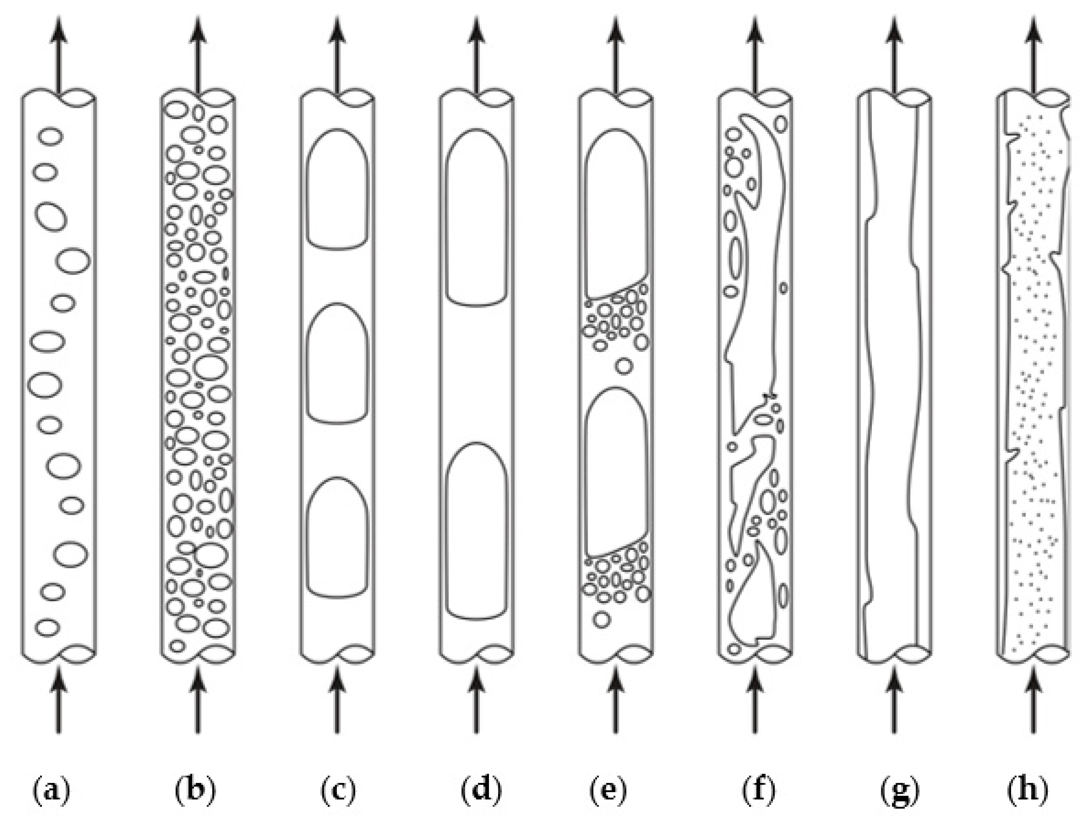
- Slug regime; when the interfacial tension is greater than inertial forces, and the Weber numbers are and .
- Monodispersed droplet regime; when the carrier phase flow rate is increased, and the Weber numbers.
- The droplet population regime; when and . This flow regime is observed at the center of the channel where the inertial effects of the continuous phase are significantly greater than the interfacial tension.
- Chaotic thin striations regime; when both flow rates are increased the We numbers are in a range of and . This flow map will be eventually changed into annular due to the instability of the flow.
4.2. Numerical Simulations
5. Flow Regime Transitions
6. Slug Length
7. Pressure Drop
8. Conclusions
- The maps of Taylor flow and the transition boundaries between each flow regime have been explained by x-y graphs, where the axes are defined by the superficial phase velocities, dimensionless numbers, and volumetric flow rates.
- Most often the gas bubbles and dispersed liquid droplets are surrounded by a thin film of carrying phase, except in non-circular tubes with very high void fraction where the dry-out at the inner surface of the tube has been observed.
- There is still no universal agreement to classify all flow regimes due to the experimental apparatus and capturing equipment, which force investigators to name the flow regimes differently.
- As more efficient numerical solutions and supercomputers emerge, they are used to solve interesting microflow problems with acceptable accuracy. Since the hydrodynamic of the film thickness is crucial and informative, high-resolution images can be produced via CFD. Meanwhile, there is still room to pay more attention to this region because of the important effect of film thickness on the frictional pressure drop, bubble or droplet profile, and heat and mass transfer.
- Contact angle can play a major role in the flow pattern as long as two phases are in contact with the inner surface of the tube, except for Taylor flow is, i.e., gas bubbles or dispersed liquid droplets surrounded by a liquid film.
- The transition criterion from one flow regime into another one has been investigated by many researchers, resulting in numerous criteria based on the nature of the flow, experimental approach, and key parameters.
- The quantitative attempts to correlate slug length, liquid film thickness (recently summarized by [4] in a comprehensive review paper), and pressure drop have been compared. These correlations include non-dimensional numbers, superficial velocity ratios, volumetric flow rate ratios, void fraction, and other thermophysical characteristics of phases.
Author Contributions
Funding
Institutional Review Board Statement
Informed Consent Statement
Data Availability Statement
Conflicts of Interest
Nomenclature
| Dimensionless numbers (discussed in the text) | ||
| Ar | Archimedes number | |
| Bo | Bond number | |
| Ca | Capillary number | |
| Cn | Cahn number | |
| Eo | Eötvös number | |
| Fr | Froude number | |
| La | Laplace number | |
| N | viscosity number | |
| Oh | Ohnesorge number | |
| Re | Reynolds number | |
| Su | Suratman number | |
| We | Weber number | |
| English letters | ||
| A | [m2] | area of the channel |
| A | [micron] | microreactor oscillation in Equation (9) |
| B | [lb hr−1 ft−2] | mass velocity of the liquid phase |
| C | [–] | Chisholm constant (5, 10, 15, and 20 for different flow regimes) |
| d | [m] | tube diameter |
| f | [–] | friction factor and a function defined by Wang et al. [179] |
| [kHz] | constant vibrating frequency | |
| [–] | a function defined by Wang et al. [179] | |
| F | [s−1] | frequency of gas bubbles |
| g | [m s−2] | gravity acceleration |
| G | [lb hr−1 ft−2] | mass velocity of the gas phase |
| h | [mm] | the height of the rectangular cross-sectional area channel |
| H | [m] | Kelvin-Helmholtz instability index |
| K | [–] | end effect of a bubble |
| j | [ms−1] | superficial velocity in Figure 6 |
| L | [m] | length |
| [kg s−1] | mass flow rate | |
| n | [–] | number of slugs |
| p | [Nm−2] | pressure |
| Q | [ml s−1] | volumetric flow rate |
| r | [m] | radial distance from the axis of the tube |
| R | [m] | radius of channel, equivalent radius in Equation (6) |
| s | [–] | channel gap |
| S | [–] | slip ratio |
| t | [s] | time |
| U | [ms−1] | average velocity |
| v | [volt] | voltage |
| V | [ms−1] | superficial velocity |
| w | [mm] | the width of the rectangular channel |
| x | [–] | the quality or the dryness fraction |
| X | [–] | Lockhart-Martinelli parameter |
| z | [m] | axial length (m) |
| Greek letters | ||
| α | [–] | void fraction |
| β | [–] | the volumetric quality |
| γ | [–] | the ratio between the dynamic viscosity of droplet to continuous phase |
| δ | [m] | liquid film thickness |
| ε | [–] | the gas phase holdup |
| λ | ||
| µ | [Pa.s] | dynamic viscosity |
| ν | the volume of liquid flowing per bubble and slug | |
| ξ | [m] | interface width |
| ρ | [kgm−3] | density |
| σ | [Nm−1] | interfacial tension |
| [s−1] | angular frequency | |
| [mm3] | volume of the dispersed phase | |
| φ | [–] | two-phase friction multiplier |
| ψ | ||
| Δ | [–] | gradient operator |
| Subscripts and superscripts | ||
| * | minimum or maximum, and dimensionless parameters | |
| 0 | initial | |
| 3D | droplet at the junction | |
| a | aqueous phase | |
| b | the equivalent diameter of a sphere | |
| b | bubble | |
| c | continuous | |
| ca | capillary | |
| cap | head or rear meniscuses of the gas bubble | |
| CH1 | the first detection point | |
| CH2 | the second detection point | |
| cr | critical | |
| d | dispersed | |
| D | diagonal direction in Figure 10 | |
| f | film | |
| g | gas | |
| H | hydraulic | |
| i | interfacial | |
| l | liquid | |
| L | lateral direction in Figure 10 | |
| ks | kerosene-superficial | |
| m | mixture or mean | |
| max | maximum | |
| mf | moving film | |
| min | minimum | |
| o | organic phase | |
| rec | receding | |
| s | slug | |
| sf | stagnant film | |
| s∞ | the radius of the gas bubble in the uniform film thickness region | |
| t | total | |
| th | macro-to-micro-scale threshold | |
| tp | two-phase velocity | |
| uc | unit cell | |
| ws | water-superficial | |
| Acronyms | ||
| FEP | fluorinated ethylene propylene | |
| GL | gas–liquid | |
| LBM | lattice Boltzmann method | |
| LL | liquid–liquid | |
| probability density function | ||
| VoF | volume of fluid | |
| XFVM | extended finite volume method | |
| μ-PIV | micro-particle image velocimetry | |
References
- Angeli, P.; Gavriilidis, A. Hydrodynamics of Taylor flow in small channels: A review. J. Mech. Eng. Sci. 2008, 222, 737–751. [Google Scholar] [CrossRef]
- Awad, M.M.; Muzychka, Y.S. Two-phase flow modeling in microchannels and minichannels. Heat Transfer Eng. 2010, 31, 1023–1033. [Google Scholar] [CrossRef]
- Awad, M.M.; Muzychka, Y.S. Effective property models for homogeneous two-phase flows. Exp. Therm. Fluid Sci. 2008, 33, 106–113. [Google Scholar] [CrossRef]
- Etminan, A.; Muzychka, Y.S.; Pope, K. Liquid film thickness of two-phase slug flows in capillary microchannels: A review paper. Can. J. Chem. Eng. 2021, 1, 1–24. [Google Scholar] [CrossRef]
- Awad, M.M. Two-phase flow. In An Overview of Heat Transfer Phenomena; Salim, N.K., Ed.; IntechOpen: London, UK, 2012. [Google Scholar] [CrossRef]
- Turton, R.; Clark, N.N. An explicit relationship to predict spherical particle terminal velocity. Powder Technol. 1987, 53, 127–129. [Google Scholar] [CrossRef]
- Hua, J.; Quan, S.; Nossen, J. Numerical simulation of an intermediate sized bubble rising in a vertical pipe. Comp. Meth. Multiph. Flow 2009, 63, 111–121. [Google Scholar] [CrossRef] [Green Version]
- Yin, X.; Koch, D.L. Hindered settling velocity and microstructure in suspensions of solid spheres with moderate Reynolds numbers. Phys. Fluids 2007, 19, 093302. [Google Scholar] [CrossRef]
- Zhang, Q.; Prosperetti, A. Physics-based analysis of the hydrodynamic stress in a fluid-particle system. Phys. Fluids 2010, 22, 033306. [Google Scholar] [CrossRef] [Green Version]
- Zhan, C.; Sardina, G.; Lushi, E.; Brandt, L. Accumulation of motile elongated micro-organisms in turbulence. J. Fluid Mech. 2014, 739, 22–36. [Google Scholar] [CrossRef] [Green Version]
- Rabinovich, E.; Kalman, H. Pickup, critical and wind threshold velocities of particles. Powder Technol. 2007, 176, 9–17. [Google Scholar] [CrossRef]
- Quan, S. Co-current flow effects on a rising Taylor bubble. Int. J. Multiph. Flow 2011, 37, 888–897. [Google Scholar] [CrossRef]
- Uno, S.; Kintner, R.C. Effect of wall proximity on the rate of rise of single air bubbles in a quiescent liquid. AIChE J. 1956, 2, 420–425. [Google Scholar] [CrossRef]
- Li, W.; Wu, Z. A general criterion for evaporative heat transfer in micro/mini-channels. Int. J. Heat Mass Tranf. 2010, 53, 1967–1976. [Google Scholar] [CrossRef]
- Li, W.; Wu, Z. A general correlation for adiabatic two-phase pressure drop in micro/mini-channels. Int. J. Heat Mass Tranf. 2010, 53, 2732–2739. [Google Scholar] [CrossRef]
- Wu, Z.; Li, W. A new predictive tool for saturated critical heat flux in micro/mini–channels: Effect of the heated length-to-diameter ratio. Int. J. Heat Mass Tranf. 2010, 54, 2880–2889. [Google Scholar] [CrossRef]
- Wu, Z.; Li, W.; Ye, S. Correlations for saturated critical heat flux in micro-channels. Int. J. Heat Mass Tranf. 2010, 54, 379–389. [Google Scholar] [CrossRef]
- Ganapathy, H.; Shooshtari, A.; Dessiatoun, S.; Alshehhi, M.; Ohadi, M. Fluid flow and mass transfer characteristics of enhanced CO2 capture in a minichannel reactor. Appl. Energ. 2014, 119, 43–56. [Google Scholar] [CrossRef]
- Prajapati, Y.K.; Bhandari, P. Flow boiling instabilities in microchannels and their promising solutions—A review. Exp. Therm. Fluid Sci. 2017, 88, 576–593. [Google Scholar] [CrossRef]
- Cahn, J.W.; Hilliard, J.E. Free energy of a nonuniform system. I. interfacial free energy. J. Chem. Phys. 1958, 28, 258–267. [Google Scholar] [CrossRef]
- Cahn, J.W.; Hilliard, J.E. Free energy of a nonuniform system. III. nucleation in a two-component incompressible fluid. J. Chem. Phys. 1959, 31, 688–699. [Google Scholar] [CrossRef]
- Cahn, J.W. Free energy of a nonuniform system. II. thermodynamic basis. J. Chem. Phys. 1959, 30, 1121–1123. [Google Scholar] [CrossRef]
- Cahn, J.W. On spinodal decomposition. Acta Metal. 1961, 9, 795–801. [Google Scholar] [CrossRef]
- Langer, J.S. Spinodal decomposition. In Fluctuations, Instabilities, and Phase Transitions; NATO Advanced Study Institutes Series (Series B: Physics); Springer: Boston, MA, USA, 1975. [Google Scholar] [CrossRef]
- Anderson, D.M.; McFadden, G.B. Diffuse-interface methods in fluid mechanics. Annu. Rev. Fluid Mech. 1998, 30, 139–165. [Google Scholar] [CrossRef] [Green Version]
- He, Q.; Hasegawa, Y.; Kasagi, N. Heat transfer modelling of gas-liquid slug flow without phase change in a micro tube. Int. J. Heat Fluid Flow 2010, 31, 126–136. [Google Scholar] [CrossRef]
- Choi, Y.J.; Anderson, P.D. Cahn-Hillard modelling of particles suspended in two-phase flows. Int. J. Numer. Meth. Fluids 2011, 69, 995–1015. [Google Scholar] [CrossRef]
- Fairbrother, F.; Stubbs, A.E. Studies in electro-endosmosis: Part VI. The “bubble-tube” method of measurement. J. Chem. Soc. 1935, 1, 527–529. [Google Scholar] [CrossRef]
- Marchessault, R.N.; Mason, S.G. Flow of entrapped bubbles through a capillary. Ind. Eng. Chem. 1960, 52, 79–84. [Google Scholar] [CrossRef]
- Bretherton, F.P. The motion of long bubbles in tubes. J. Fluid Mech. 1961, 10, 166–188. [Google Scholar] [CrossRef]
- Taylor, G.I. Deposition of a viscous fluid on the wall of a tube. J. Fluid Mech. 1961, 10, 161–165. [Google Scholar] [CrossRef]
- Schwartz, L.W.; Princen, H.M.; Kiss, A.D. On the motion of bubbles in capillary tubes. J. Fluid Mech. 1986, 172, 259–275. [Google Scholar] [CrossRef]
- Teletzke, G.F.; Davis, H.T.; Scriven, L.E. Wetting hydrodynamics. Rev. Phys. Appl. 1988, 23, 989–1007. [Google Scholar] [CrossRef]
- Irandoust, S.; Andersson, B. Simulation of flow and mass transfer in Taylor flow through a capillary. Compu. Chem. Eng. 1989, 13, 519–526. [Google Scholar] [CrossRef]
- Ratulowski, J.; Chang, H.C. Transport of gas bubbles in capillaries. Phys. Fluids A Fluid Dyn. 1989, 1, 1642–1655. [Google Scholar] [CrossRef]
- Giavedoni, M.D.; Saita, F.A. The axisymmetric and plane cases of a gas phase steadily displacing a Newtonian liquid–A simultaneous solution of the governing equations. Phys. Fluids 1997, 9, 2420–2428. [Google Scholar] [CrossRef]
- Thulasidas, T.C.; Abraham, M.A.; Cerro, R.L. Flow patterns in liquid slugs during bubble-train flow inside capillaries. Chem. Eng. Sci. 1997, 52, 2947–2962. [Google Scholar] [CrossRef]
- Giavedoni, M.D.; Saita, F.A. The rear meniscus of a long bubble steadily displacing a Newtonian liquid in a capillary tube. Phys. Fluids 1999, 11, 786–794. [Google Scholar] [CrossRef]
- Heiszwolf, J.J.; Engelvaart, L.B.; Gvd Eijnden, M.; Kreutzer, M.T.; Kapteijn, F.; Moulijn, J.A. Hydrodynamic aspects of the monolithic loop reactor. Chem. Eng. Sci. 2001, 56, 805–812. [Google Scholar] [CrossRef]
- Aussillous, P.; Quéré, D. Quick deposition of a fluid on the wall of a Tube. Phys. Fluids 2000, 12, 2367–2371. [Google Scholar] [CrossRef]
- Bico, J.; Quéré, D. Liquid trains in a tube. Europhys. Lett. 2000, 51, 546–550. [Google Scholar] [CrossRef]
- Kreutzer, M.T.; Du, P.; Heiszwolf, J.J.; Kapteijn, F.; Moulijn, J.A. Mass transfer characteristics of three-phase monolith reactors. Chem. Eng. Sci. 2001, 56, 6015–6023. [Google Scholar] [CrossRef]
- Heil, M. Finite Reynolds number effects in the Bretherton problem. Phys. Fluids 2001, 13, 2517–2521. [Google Scholar] [CrossRef]
- Kreutzer, M.T.; Kapteijn, F.; Moulijn, J.A.; Heiszwolf, J.J. Multiphase monolith reactors: Chemical reaction engineering of segmented flow in microchannels. Chem. Eng. Sci. 2005, 60, 5895–5916. [Google Scholar] [CrossRef]
- Grimes, R.; King, C.; Walsh, E. Film thickness for two phase flow in a microchannel. In Proceedings of the ASME 2006 International Mechanical Engineering Congress and Exposition, Chicago, IL, USA, 5–10 November 2006; pp. 207–211. [Google Scholar] [CrossRef]
- Han, Y.; Shikazono, N. Measurement of the liquid film thickness in micro tube slug flow. Int. J. Heat Fluid Flow 2009, 30, 842–853. [Google Scholar] [CrossRef]
- Eain, M.M.G.; Egan, V.; Punch, J. Film thickness measurements in liquid-liquid slug flow regimes. Int. J. Heat Fluid Flow 2013, 44, 515–523. [Google Scholar] [CrossRef] [Green Version]
- Gupta, R.; Leung, S.S.Y.; Manica, R.; Fletcher, D.F.; Haynes, B.S. Hydrodynamics of liquid-liquid Taylor flow in microchannels. Chem. Eng. Sci. 2013, 92, 180–189. [Google Scholar] [CrossRef]
- Klaseboer, E.; Gupta, R.; Manica, R. An extended Bretherton model for long Taylor bubbles at moderate capillary Numbers. Phys. Fluids 2014, 26, 032107. [Google Scholar] [CrossRef]
- Huang, H.; Dhir, V.K.; Pan, L.M. Liquid film thickness measurement underneath a gas slug with miniaturized sensor matrix in a microchannel. Microfluid Nanofluid 2017, 21, 159. [Google Scholar] [CrossRef]
- Ni, D.; Hong, F.J.; Cheng, P.; Chen, G. Numerical study of liquid-gas and liquid-liquid Taylor flows using a two-phase flow model based on Arbitrary-Lagrangian-Eulerian (ALE) Formulation. Int. Commun. Heat Mass 2017, 88, 37–47. [Google Scholar] [CrossRef]
- Patel, R.S.; Weibel, J.A.; Garimella, S.V. Characterization of liquid film thickness in slug-regime microchannel flows. Int. J. Heat Mass Tranf. 2017, 115, 1137–1143. [Google Scholar] [CrossRef] [Green Version]
- Kreutzer, M.T.; van der Eijnden, M.G.; Kapteijn, F.; Moulijn, J.A.; Heiszwolf, J.J. The pressure drop experiment to determine slug lengths in multiphase monoliths. Catal. Today 2005, 105, 667–672. [Google Scholar] [CrossRef]
- Walsh, E.; Muzychka, Y.S.; Walsh, P.; Egan, V.; Punch, J. Pressure drop in two phase slug/bubble flows in mini scale capillaries. Int. J. Multiph. Flow 2009, 35, 879–884. [Google Scholar] [CrossRef]
- Warnier, M.J.F.; de Croon, M.H.J.M.; Rebrov, E.V.; Schouten, J.C. Pressure drop of gas-liquid Taylor flow in round micro-capillaries for low to intermediate Reynolds numbers. Microfluid Nanofluid 2010, 8, 33–45. [Google Scholar] [CrossRef] [Green Version]
- Jovanović, J.; Zhou, W.; Rebrov, E.V.; Nijhuis, T.A.; Hessel, V.; Schouten, J.C. Liquid-liquid slug flow: Hydrodynamics and pressure drop. Chem. Eng. Sci. 2011, 66, 42–54. [Google Scholar] [CrossRef]
- Eain, M.M.G.; Egan, V.; Howard, J.; Walsh, P.; Walsh, E.; Punch, J. Review and extension of pressure drop models applied to Taylor flow regimes. Int. J. Multiph. Flow 2015, 68, 1–9. [Google Scholar] [CrossRef] [Green Version]
- Qian, D.; Lawal, A. Numerical study on gas and liquid slugs for Taylor flow in a T-junction microchannel. Chem. Eng. Sci. 2006, 61, 7609. [Google Scholar] [CrossRef]
- Tan, J.; Xu, J.H.; Li, S.W.; Luo, G.S. Drop dispenser in a cross-junction microfluidic device: Scaling and mechanism of break-up. Chem. Eng. J. 2008, 136, 306–311. [Google Scholar] [CrossRef]
- Fries, D.M.; von Rohr, P.R. Liquid mixing in gas-liquid two-phase flow by meandering microchannels. Chem. Eng. Sci. 2009, 64, 1326–1335. [Google Scholar] [CrossRef]
- Steegmans, M.L.J.; Schroën, K.G.P.H.; Boom, R.M. Characterization of emulsification at flat microchannel Y junctions. Langmuir 2009, 25, 3396–3401. [Google Scholar] [CrossRef]
- White, F.M. Viscous Fluid Flow, 3rd ed.; McGraw–Hill: New York, NY, USA, 2006. [Google Scholar]
- White, F.M. Fluid Mechanics, 8th ed.; McGraw–Hill: New York, NY, USA, 2016. [Google Scholar]
- Suo, M.; Griffith, P. Two-phase flow in capillary tube. J. Basic Eng. 1964, 86, 576–582. [Google Scholar] [CrossRef] [Green Version]
- Jayawardena, S.S.; Balakotaiah, V.; Witte, L.C. Flow pattern transition maps for microgravity two-phase flows. AIChE J. 1997, 43, 1637–1640. [Google Scholar] [CrossRef]
- Hewitt, G.F.; Roberts, D.N. Studies of Two-Phase Flow Patterns by Simultaneous X-Ray and Flash Photography. Atomic Energy Research Establishment, Harwell, England, AERE–M 2159. 1969. Available online: https://www.osti.gov/servlets/purl/4798091 (accessed on 5 January 2021).
- Fukano, T.; Kariyasaki, A. Characteristics of gas-liquid two-phase flow in a capillary tube. Nucl. Eng. Des. 1993, 141, 59–68. [Google Scholar] [CrossRef]
- Triplett, K.A.; Ghiaasiaan, S.M.; Abdel–Khalik, S.I.; Sadowskia, D.L. Gas-liquid two-phase flow in microchannels Part I: Two-phase flow patterns. Int. J. Multiph. Flow 1999, 25, 377–394. [Google Scholar] [CrossRef]
- Zhao, T.S.; Bi, Q.C. Co–current air-water two-phase flow patterns in vertical triangular microchannels. Int. J. Multiph. Flow 2001, 27, 765–782. [Google Scholar] [CrossRef]
- Akbar, M.K.; Plummer, D.A.; Ghiaasiaan, S.M. Gas-liquid two-phase flow regimes in microchannels. In Proceedings of the ASME International Mechanical Engineering Congress and Exposition, New Orleans, LO, USA, 17–22 November 2002; pp. 527–534. [Google Scholar] [CrossRef]
- Kawaji, M.; Chung, P.M.-Y. Unique characteristics of adiabatic gas-liquid flows in microchannels: Diameter and shape effects on flow patterns, void fraction and pressure drop. In Proceedings of the ASME 1st International Conference on Microchannels and Minichannels, Rochester, NY, USA, 24–25 April 2003; pp. 115–127. [Google Scholar] [CrossRef]
- Cubaud, T.; Ho, C.M. Transport of bubbles in square microchannels. Phys. Fluids 2004, 16, 4575–4585. [Google Scholar] [CrossRef]
- Günther, A.; Khan, S.A.; Thalmann, M.; Trachsel, F.; Jensen, K.F. Transport and reaction in microscale segmented gas-liquid Flow. Lab. Chip 2004, 4, 278–286. [Google Scholar] [CrossRef]
- Yue, J.; Chen, G.; Yuan, Q.; Luo, L.; Gonthier, Y. Hydrodynamics and mass transfer characteristics in gas-liquid flow through a rectangular microchannel. Chem. Eng. Sci. 2007, 62, 2096–2108. [Google Scholar] [CrossRef]
- Kirpalani, D.M.; Patel, T.; Mehrani, P.; Macchi, A. Experimental analysis of the unit cell approach for two-phase flow dynamics in curved flow channels. Int. J. Heat Mass Tranf. 2008, 51, 1095–1103. [Google Scholar] [CrossRef]
- Yue, J.; Luo, L.; Gonthier, Y.; Chen, G.; Yuan, Q. An experimental investigation of gas-liquid two-phase flow in single microchannel contactors. Chem. Eng. Sci. 2008, 63, 4189–4202. [Google Scholar] [CrossRef]
- Dessimoz, A.L.; Raspail, P.; Berguerand, C.; Kiwi–Minsker, L. Quantitative criteria to define flow patterns in micro-capillaries. Chem. Eng. J. 2010, 160, 882–890. [Google Scholar] [CrossRef]
- Roudet, M.; Loubiere, K.; Gourdon, C.; Cabassud, M. Hydrodynamic and mass transfer in inertial gas-liquid flow regimes through straight and meandering millimetric square channels. Chem. Eng. Sci. 2011, 66, 2974–2990. [Google Scholar] [CrossRef] [Green Version]
- Deendarlianto; Rahmandhika, A.; Widyatama, A.; Dinaryanto, O.; Widyaparaga, A.; Indarto. Experimental study on the hydrodynamic behavior of gas-liquid air-water two-phase flow near the transition to slug flow in horizontal pipes. Int. J. Heat Mass Tranf. 2019, 130, 187–203. [Google Scholar] [CrossRef]
- Wu, Z.; Sundén, B. Liquid-liquid two-phase flow patterns in ultra-shallow straight and serpentine microchannels. Heat Mass Transfer 2019, 55, 1095–1108. [Google Scholar] [CrossRef] [Green Version]
- Farokhpoor, R.; Liu, L.; Langsholt, M.; Hald, K.; Amundsen, J. Dimensional analysis and scaling in two-phase gas-liquid stratified pipe flow-methodology evaluation. Int. J. Multiph. Flow 2020, 122, 103139. [Google Scholar] [CrossRef]
- Zhao, Y.; Chen, G.; Yuan, Q. Liquid-liquid two-phase flow patterns in a rectangular microchannel. AIChE J. 2006, 52, 4052–4060. [Google Scholar] [CrossRef]
- Yagodnitsyna, A.A.; Kovalev, A.V.; Bilsky, A.V. Flow patterns of immiscible liquid-liquid flow in a rectangular microchannel with T-junction. Chem. Eng. J. 2016, 303, 547–554. [Google Scholar] [CrossRef]
- Baker, O. Design of pipelines for the simultaneous flow of oil and gas. In Proceedings of the Fall Meeting of the Petroleum Branch of AIME, Dallas, TX, USA, 19–21 October 1953; p. 323-G. [Google Scholar] [CrossRef]
- Sato, T.; Minamiyama, T.; Yanai, M.; Tokura, T.; Ito, Y. Study of heat transfer in boiling two-phase channel flow Part II, Heat transfer in the nucleate boiling region. Heat Tran. Jap. Res. 1972, 1, 15–30. [Google Scholar]
- Cubaud, T.; Mason, T.G. Capillary threads and viscous droplets in square microchannels. Phys. Fluids 2008, 20, 053302. [Google Scholar] [CrossRef] [Green Version]
- Akbar, M.K.; Plummer, D.A.; Ghiaasiaan, S.M. On gas-liquid two-phase flow regimes in microchannels. Int. J. Multiph. Flow 2003, 29, 855–865. [Google Scholar] [CrossRef]
- Kreutzer, M.T.; Kapteijn, F.; Moulijn, J.A.; Kleijn, C.R.; Heiszwolf, J.J. Inertial and interfacial effects on pressure drop of Taylor flow in capillaries. AIChE J. 2005, 51, 2428–2440. [Google Scholar] [CrossRef]
- Tsaoulidis, D.; Dore, V.; Angeli, P.; Plechkova, N.V.; Seddon, K.R. Flow patterns and pressure drop of ionic liquid-water two-phase flows in microchannels. Int. J. Multiph. Flow 2013, 54, 1–10. [Google Scholar] [CrossRef] [Green Version]
- Wright, R. Jamin effect in oil production. AAPG Bull. 1934, 18, 548–549. [Google Scholar] [CrossRef]
- Gibbs, J.W. On the equilibrium of heterogeneous substances. Am. J. Sci. 1878, 16, 441–458. [Google Scholar] [CrossRef]
- Wallis, G.B. The Transition from Flooding to Upwards Concurrent Annular Flow in a Vertical Pipe; UKAEA Report, AEEW–R–142; United Kingdom Atomic Energy Authority: Abingdon, UK, 1962.
- Dore, V.; Tsaoulidis, D.; Angeli, P. Mixing patterns in water plugs during water/ionic liquid segmented flow in microchannels. Chem. Eng. Sci. 2012, 80, 334–341. [Google Scholar] [CrossRef] [Green Version]
- Meyer, C.; Hoffmann, M.; Schlüter, M. Micro-PIV analysis of gas–liquid Taylor flow in a vertical oriented square shaped fluidic channel. Int. J. Multiph. Flow 2014, 67, 140–148. [Google Scholar] [CrossRef]
- Aland, S.; Lehrenfeld, C.; Marschall, H.; Meyer, C.; Weller, S. Accuracy of two phase flow simulations: The Taylor flow benchmark. In Proceedings of the 84th Annual Meeting of the International Association of Applied Mathematics and Mechanics (GAMM), Novi Sad, Serbia, 18 March 2013; pp. 595–598. [Google Scholar] [CrossRef]
- Kong, R.; Kim, S.; Bajorek, S.; Tien, K.; Hoxie, C. Effects of pipe size on horizontal two-phase flow: Flow regimes, pressure drop, two-phase flow parameters, and drift–flux analysis. Exp. Therm. Fluid Sci. 2018, 96, 75–89. [Google Scholar] [CrossRef]
- Butler, C.; Lalanne, B.; Sandmann, K.; Cid, E.; Billet, A.M. Mass transfer in Taylor flow: Transfer rate modelling from measurements at the slug and film scale. Int. J. Multiph. Flow 2018, 105, 185–201. [Google Scholar] [CrossRef] [Green Version]
- Yao, C.; Ma, H.; Zhao, Q.; Liu, Y.; Zhao, Y.; Chen, G. Mass transfer in liquid-liquid Taylor flow in a microchannel: Local concentration distribution, mass transfer regime and the effect of fluid viscosity. Chem. Eng. Sci. 2020, 223, 115734. [Google Scholar] [CrossRef]
- Kew, P.A.; Cornwell, K. Correlations for the prediction of boiling heat transfer in small-diameter channels. Appl. Therm. Eng. 1997, 17, 705–715. [Google Scholar] [CrossRef]
- Cubaud, T.; Ulmanella, U.; Ho, C.M. Two-phase flow in microchannels with surface modifications. Fluid Dyn. Res. 2006, 38, 772–786. [Google Scholar] [CrossRef]
- Kashid, M.N.; Agar, D.W. Hydrodynamics of liquid–liquid slug flow capillary microreactor: Flow regimes, slug size and pressure drop. Chem. Eng. J. 2007, 131, 1–13. [Google Scholar] [CrossRef]
- Kashid, M.N.; Harshe, Y.M.; Agar, D.W. Liquid-liquid slug flow in a capillary: An alternative to suspended drop or film contactors. Ind. Eng. Chem. Res. 2007, 46, 8420–8430. [Google Scholar] [CrossRef]
- Steijn, V.V.; Kreutzerb, M.T.; Kleijn, C.R. μ-PIV study of the formation of segmented flow in microfluidic T-junctions. Chem. Eng. Sci. 2007, 62, 7505–7514. [Google Scholar] [CrossRef]
- Harirchian, T.; Garimella, S.V. The critical role of channel cross-sectional area in microchannel flow boiling heat transfer. Int. J. Multiph. Flow 2009, 35, 904–913. [Google Scholar] [CrossRef] [Green Version]
- Niu, H.; Pan, L.; Su, H.; Wang, S. Flow pattern, pressure drop, and mass transfer in a gas-liquid concurrent two-phase flow microchannel reactor. Ind. Eng. Chem. Res. 2009, 48, 1621–1628. [Google Scholar] [CrossRef]
- Kashid, M.N.; Fernández Rivas, D.; Agar, D.W.; Turek, S. On the hydrodynamics of liquid-liquid slug flow capillary microreactors. Asia-Pac. J. Chem. Eng. 2008, 3, 151–160. [Google Scholar] [CrossRef]
- Fouilland, T.S.; Fletcher, D.F.; Haynes, B.S. Film and slug behaviour in intermittent slug–annular microchannel flows. Chem. Eng. Sci. 2010, 65, 5344–5355. [Google Scholar] [CrossRef]
- Ong, C.L.; Thome, J.R. Macro-to-microchannel transition in two-phase flow: Part 1–Two phase flow patterns and film thickness measurements. Exp. Therm. Fluid Sci. 2011, 35, 37–47. [Google Scholar] [CrossRef]
- Khaledi, H.A.; Smith, I.E.; Unander, T.E.; Nossen, J. Investigation of two-phase flow pattern, liquid holdup and pressure drop in viscous oil-gas flow. Int. J. Multiph. Flow 2014, 67, 37–51. [Google Scholar] [CrossRef]
- Gubbins, K.E.; Moore, J.D. Molecular modeling of matter: Impact and prospects in engineering. Ind. Eng. Chem. Res. 2010, 49, 3026–3046. [Google Scholar] [CrossRef]
- Wörner, M. Numerical modeling of multiphase flows in microfluidics and micro process engineering: A review of methods and applications. Microfluid Nanofluid 2012, 12, 841–886. [Google Scholar] [CrossRef]
- Keyes, D.E.; McInnes, L.C.; Woodward, C.; Gropp, W.; Myra, E.; Pernice, M.; Bell, J. Multiphysics simulations: Challenges and opportunities. Int. J. High. Perform. C 2013, 27, 4–83. [Google Scholar] [CrossRef] [Green Version]
- Hashim, U.; Diyana, P.N.A.; Adam, T. Numerical simulation of microfluidic devices. In Proceedings of the 10th IEEE International Conference on Semiconductor Electronics (ICSE), Kuala Lumpur, Malaysia, 19–21 September 2012; pp. 26–29. [Google Scholar] [CrossRef]
- Apte, S.V.; Mahesh, K.; Lundgren, T. A Eulerian-Lagrangian Model to Simulate Two-Phase/Particulate Flows. Center for Turbulence Research, Center for Turbu-lence Research, Annual Research Briefs. 2003, pp. 161–171. Available online: https://apps.dtic.mil/sti/citations/ADP014800 (accessed on 5 January 2021).
- Trapp, J.A.; Mortensen, G.A. A discrete particle model for bubble slug two-phase flow. J. Comput. Phy. 1993, 107, 367–377. [Google Scholar] [CrossRef]
- Delnoij, E.; Lammers, F.A.; Kuipers, J.A.M.; van Swaaij, W.P.M. Dynamic simulation of dispersed gas-liquid two-phase flow using a discrete bubble model. Chem. Eng. Sci. 1997, 52, 1429–1458. [Google Scholar] [CrossRef] [Green Version]
- Ye, M.; Van Der Hoef, M.A.; Kuipers, J.A.M. From discrete particle model to a continuous model of Geldart a particles. Chem. Eng. Res. Des. 2005, 83, 833–843. [Google Scholar] [CrossRef] [Green Version]
- Pepiot, P.; Desjardins, O. Numerical analysis of the dynamics of two-and three-dimensional fluidized bed reactors using an Euler-Lagrange approach. Powder Technol. 2012, 220, 104–121. [Google Scholar] [CrossRef]
- Barbosa, M.V.; De Lai, F.C.; Junqueira, S.L.M. Numerical evaluation of CFD-DEM coupling applied to lost circulation control: Effects of particle and flow inertia. Math. Prob. Eng. 2019, 1–13. [Google Scholar] [CrossRef]
- Chen, S.; Doolen, G.D. Lattice Boltzmann method for fluid flows. Annu. Rev. Fluid Mech. 1998, 30, 329–364. [Google Scholar] [CrossRef] [Green Version]
- Frisch, U.; Hasslacher, B.; Pomeau, Y. Lattice-gas automata for the Navier-Stokes equation. Phys. Rev. Lett. 1986, 56, 1505–1508. [Google Scholar] [CrossRef] [PubMed] [Green Version]
- McNamara, G.R.; Zanetti, G. Use of the Boltzmann equation to simulate lattice-gas automata. Phys. Rev. Lett. 1988, 61, 2332–2335. [Google Scholar] [CrossRef]
- Chen, S.; Chen, H.; Martnez, D.; Matthaeus, W. Lattice Boltzmann model for simulation of magnetohydrodynamics. Phys. Rev. Lett. 1991, 67, 3776–3779. [Google Scholar] [CrossRef] [PubMed]
- Gunstensen, A.K.; Rothman, D.H. Lattice Boltzmann model of immiscible fluids. Phys. Rev. A 1991, 43, 4320–4327. [Google Scholar] [CrossRef] [PubMed]
- Grunau, D.; Chen, S.; Eggert, K. A lattice Boltzmann model for multiphase fluid flows. Phys. Fluids A Fluid 1993, 5, 2557–2562. [Google Scholar] [CrossRef] [Green Version]
- Shan, X.; Chen, H. Lattice Boltzmann model for simulating flows with multiple phases and components. Phys. Rev. A 1993, 47, 1815–1819. [Google Scholar] [CrossRef] [PubMed] [Green Version]
- Takada, N.; Misawa, M.; Tomiyama, A.; Fujiwara, S. Numerical simulation of two- and three-dimensional two-phase fluid motion by lattice Boltzmann method. Comput. Phys. Commun. 2000, 129, 233–246. [Google Scholar] [CrossRef]
- Inamuro, T.; Miyahara, T.; Ogino, F. Lattice Boltzmann simulations of drop deformation and breakup in a simple shear flow. In Computational Fluid Dynamics 2000; Satofuka, N., Ed.; Springer: Berlin/Heidelberg, Germany, 2001; pp. 499–504. [Google Scholar] [CrossRef]
- Seta, T.; Kono, K. Thermal lattice Boltzmann method for liquid-gas two-phase flows in two dimension. JSME Int. J. Ser. B Fluids Therm. Eng. 2004, 47, 572–583. [Google Scholar] [CrossRef] [Green Version]
- Komrakova, A.E.; Shardt, O.; Eskin, D.; Derksen, J.J. Lattice Boltzmann simulations of drop deformation and breakup in shear flow. Int. J. Multiph. Flow 2014, 59, 24–43. [Google Scholar] [CrossRef]
- Li, Q.; Luo, K.H.; Kang, Q.J.; He, Y.L.; Chen, Q.; Liu, Q. Lattice Boltzmann methods for multiphase flow and phase-change heat transfer. Prog. Energ. Combust. 2016, 52, 62–105. [Google Scholar] [CrossRef] [Green Version]
- Fei, L.; Du, J.; Luo, K.H.; Succi, S.; Lauricella, M.; Montessori, A.; Wang, Q. Modeling realistic multiphase flows using a non-orthogonal multiple-relaxation-time lattice Boltzmann method. Phys. Fluids 2019, 31, 042105. [Google Scholar] [CrossRef]
- Qin, F.; Mazloomi Moqaddam, A.; Kang, Q.; Derome, D.; Carmeliet, J. Entropic multiple-relaxation-time multirange pseudopotential lattice Boltzmann model for two-phase flow. Phys. Fluids 2018, 30, 032104. [Google Scholar] [CrossRef]
- Shi, Y.; Tang, G.H.; Lin, H.F.; Zhao, P.X.; Cheng, L.H. Dynamics of droplet and liquid layer penetration in three-dimensional porous media: A lattice Boltzmann study. Phys. Fluids 2019, 31, 042106. [Google Scholar] [CrossRef]
- Cui, Y.; Wang, N.; Liu, H. Numerical study of droplet dynamics in a steady electric field using a hybrid lattice Boltzmann and finite volume method. Phys. Fluids 2019, 31, 022105. [Google Scholar] [CrossRef]
- Katopodes, N.D. Free Surface Flow Computational Methods; Butterworth-Heinemann: Oxford, UK, 2018. [Google Scholar]
- Ketabdari, M.J. Free surface flow simulation using VOF method. In Numerical Simulation-from Brain Imaging to Turbulent Flows; IntechOpen: London, UK, 2016; pp. 365–398. [Google Scholar] [CrossRef] [Green Version]
- Osher, S.; Sethian, J.A. Fronts propagating with curvature dependent speed: Algorithms based on hamilton–jacobi formulations. J. Comput. Phys. 1988, 79, 12–49. [Google Scholar] [CrossRef] [Green Version]
- Fukagata, K.; Kasagi, N.; Ua-arayaporn, P.; Himeno, T. Numerical simulation of gas-liquid two-phase flow and convective heat transfer in a micro tube. Int. J. Heat Fluid Flow 2007, 28, 72–82. [Google Scholar] [CrossRef]
- Adalsteinsson, D.; Sethian, J.A. A fast level set method for propagating interfaces. J. Comput. Phys. 1995, 118, 269–277. [Google Scholar] [CrossRef] [Green Version]
- Adalsteinsson, D.; Sethian, J.A. The fast construction of extension velocities in level set methods. J. Comput. Phys. 1999, 148, 2–22. [Google Scholar] [CrossRef]
- Mahady, K.; Afkhami, S.; Kondic, L. A volume of fluid method for simulating fluid/fluid interfaces in contact with solid boundaries. J. Comput. Phys. 2015, 294, 243–257. [Google Scholar] [CrossRef] [Green Version]
- Osher, S.; Fedkiw, R.P. Level set methods: An overview and some recent results. J. Comput. Phys. 2001, 169, 463–502. [Google Scholar] [CrossRef] [Green Version]
- Thomas, S.; Esmaeeli, A.; Tryggvason, G. Multiscale computations of thin films in multiphase flows. Int. J. Multiph. Flow 2010, 36, 71–77. [Google Scholar] [CrossRef]
- Kolb, W.B.; Cerro, R.L. The motion of long bubbles in tubes of square cross section. Phys. Fluids A Fluid 1993, 5, 1549–1557. [Google Scholar] [CrossRef]
- Berčič, G.; Pintar, A. The role of gas bubbles and liquid slug lengths on mass transport in the Taylor flow through capillaries. Chem. Eng. Sci. 1997, 52, 3709–3719. [Google Scholar] [CrossRef]
- Brauner, N.; Maron, D.M.; Rovinsky, J. A two-fluid model for stratified flows with curved interfaces. Int. J. Multiph. Flow 1998, 24, 975–1004. [Google Scholar] [CrossRef]
- Fujioka, H.; Grotberg, J.B. The steady propagation of a surfactant-laden liquid plug in a two dimensional channel. Phys. Fluids 2005, 17, 082102. [Google Scholar] [CrossRef]
- Falconi, C.J.; Lehrenfeld, C.; Marschall, H.; Meyer, C.; Abiev, R.; Bothe, D.; Reusken, A.; Schlüter, M.; Wörner, M. Numerical and experimental analysis of local flow phenomena in laminar Taylor flow in a square mini-channel. Phys. Fluids 2016, 28, 012109. [Google Scholar] [CrossRef]
- Valizadeh, K.; Farahbakhsh, S.; Bateni, A.; Zargarian, A.; Davarpanah, A.; Alizadeh, A.; Zarei, M. A parametric study to simulate the non-Newtonian turbulent flow in spiral tubes. Energy Sci. Eng. 2020, 8, 134–149. [Google Scholar] [CrossRef] [Green Version]
- Abdollahi, A.; Norris, S.E.; Sharma, R.N. Fluid flow and heat transfer of liquid-liquid Taylor flow in square microchannels. Appl. Therm Eng. 2020, 172, 115123. [Google Scholar] [CrossRef]
- Xu, F.; Yang, L.; Liu, Z.; Chen, G. Numerical investigation on the hydrodynamics of Taylor flow in ultrasonically oscillating microreactors. Chem. Eng. Sci. 2021, 235, 116477. [Google Scholar] [CrossRef]
- Kumar, V.; Vashisth, S.; Hoarau, Y.; Nigam, K.D.P. Slug flow in curved microreactors: Hydrodynamic study. Chem. Eng. Sci. 2007, 62, 7494–7504. [Google Scholar] [CrossRef]
- Goel, D.; Buwa, V.V. Numerical simulations of bubble formation and rise in microchannels. Ind. Eng. Chem. Res. 2009, 48, 8109–8120. [Google Scholar] [CrossRef]
- Gupta, R.; Fletcher, D.F.; Haynes, B.S. On the CFD modelling of Taylor flow in microchannels. Chem. Eng. Sci. 2009, 64, 2941–2950. [Google Scholar] [CrossRef]
- Gupta, R.; Fletcher, D.F.; Haynes, B.S. CFD modelling of flow and heat transfer in the Taylor flow regime. Chem. Eng. Sci. 2010, 65, 2094–2107. [Google Scholar] [CrossRef]
- Satterfield, C.N.; Ózel, F. Some characteristics of two-phase flow in monolithic catalyst structures. Ind. Eng. Chem. Fund. 1977, 16, 61–67. [Google Scholar] [CrossRef]
- Lowe, D.C.; Rezkallah, K.S. Flow regime identification in microgravity two-phase flows using void fraction signals. Int. J. Multiph. Flow 1999, 25, 433–457. [Google Scholar] [CrossRef]
- Kreutzer, M.T. Hydrodynamics of Taylor Flow in Capillaries and Monoliths Channels. Ph.D. Thesis, Delft University of Technology, Delft, The Netherlands, 2003. [Google Scholar]
- Zhang, M.; Pan, L.M.; Ju, P.; Yang, X.; Ishii, M. The mechanism of bubbly to slug flow regime transition in air-water two phase flow: A new transition criterion. Int. J. Heat Mass Tranf. 2017, 108, 1579–1590. [Google Scholar] [CrossRef]
- Bottin, M.; Berlandis, J.P.; Hervieu, E.; Lance, M.; Marchand, M.; Öztürk, O.C.; Serre, G. Experimental investigation of a developing two-phase bubbly flow in horizontal pipe. Int. J. Multiph. Flow 2014, 60, 161–179. [Google Scholar] [CrossRef]
- Govier, G.W.; Aziz, K. The Flow of Complex Mixtures in Pipes; Van Nostrand Reinhold Company: New York, NY, USA, 2008. [Google Scholar]
- Taitel, Y.; Bornea, D.; Dukler, A.E. Modelling flow pattern transitions for steady upward gas-liquid flow in vertical tubes. AIChE J. 1980, 26, 345–354. [Google Scholar] [CrossRef]
- Barnea, D.; Shoham, O.; Taitel, Y. Flow pattern transition for downward inclined two-phase flow; horizontal to Vertical. Chem. Eng. Sci. 1982, 37, 735–740. [Google Scholar] [CrossRef]
- Barnea, D.; Shoham, O.; Taitel, Y. Flow pattern transition for vertical downward two-phase flow. Chem. Eng. Sci. 1982, 37, 741–744. [Google Scholar] [CrossRef]
- Dukler, A.E.; Taitel, Y. Flow pattern transitions in gas-liquid systems: Measurement and modeling. In Multiphase Science and Technology; Springer: Berlin/Heidelberg, Germany, 1986; pp. 1–94. [Google Scholar] [CrossRef]
- Andreussi, P.; Paglianti, A.; Silva, F.S. Dispersed bubble flow in horizontal pipes. Chem. Eng. Sci. 1999, 54, 1101–1107. [Google Scholar] [CrossRef]
- Radovcich, N.A.; Moissis, R. The Transition from Two Phase Bubble Flow to Slug Flow. Department of Mechanical Engineering, Massachusetts Institute of Technology, Report No. 7–7673–22. 1962. Available online: https://dspace.mit.edu/bitstream/handle/1721.1/11439/33322807-MIT.pdf?sequence=2 (accessed on 5 January 2021).
- Mishima, K.; Ishii, M. Flow regime transition criteria for upward two-phase flow in vertical tubes. Int. J. Heat Mass Tranf. 1984, 27, 723–737. [Google Scholar] [CrossRef]
- Kelessidis, V.C.; Dukler, A.E. Modeling flow pattern transitions for upward gas-liquid flow in vertical concentric and eccentric annuli. Int. J. Multiph. Flow 1989, 15, 173–191. [Google Scholar] [CrossRef]
- Brauner, N.; Moalem Maron, D. Stability analysis of stratified liquid-liquid flow. Int. J. Multiph. Flow 1992, 18, 103–121. [Google Scholar] [CrossRef]
- Das, R.K.; Pattanayak, S. Bubble to slug flow transition in vertical upward two-phase flow through narrow tubes. Chem. Eng. Sci. 1994, 49, 2163–2172. [Google Scholar] [CrossRef]
- Cheng, H.; Hills, J.H.; Azzorpardi, B.J. A study of the bubble-to-slug transition in vertical gas-liquid flow in columns of different diameters. Int. J. Multiph. Flow 1998, 24, 431–452. [Google Scholar] [CrossRef]
- Hibiki, T.; Ishii, M. Two-group interfacial area transport equations at bubbly-to-slug flow transition. Nucl. Eng. Des. 2000, 202, 39–76. [Google Scholar] [CrossRef]
- Hibiki, T.; Mishima, K. Flow regime transition criteria for upward two-phase flow in vertical narrow rectangular channels. Nucl. Eng. Des. 2001, 203, 117–131. [Google Scholar] [CrossRef]
- Wang, T.; Wang, J.; Jin, Y. Theoretical prediction of flow regime transition in bubble columns by the population balance model. Chem. Eng. Sci. 2005, 60, 6199–6209. [Google Scholar] [CrossRef]
- Das, A.K.; Das, P.K.; Thome, J.R. Transition of bubbly flow in vertical tubes: New criteria through CFD simulation. ASME J. Fluids Eng. 2009, 131, 091303. [Google Scholar] [CrossRef]
- Das, A.K.; Das, P.K.; Thome, J.R. Transition of bubbly flow in vertical tubes: Effect of bubble size and tube diameter. ASME J. Fluids Eng. 2009, 131, 091304. [Google Scholar] [CrossRef]
- Wang, X.; Sun, X.; Doup, B.; Zhao, H. Dynamic modeling strategy for flow regime transition in gas-liquid two-phase flows. J. Comput. Multiph. Flow 2012, 4, 387–397. [Google Scholar] [CrossRef] [Green Version]
- Song, Y.; Xin, F.; Guangyong, G.; Lou, S.; Cao, C.; Wang, J. Uniform generation of water slugs in air flowing through superhydrophobic microchannels with T-junction. Chem. Eng. Sci. 2019, 199, 439–450. [Google Scholar] [CrossRef]
- Akagawa, K.; Sakaguchi, T. Fluctuation of void ratio in two-phase flow: 2nd report, analysis of flow configuration considering the existence of small bubbles in liquid slugs. Bull. JSME 1966, 9, 104–110. [Google Scholar] [CrossRef]
- Fernandes, R.C. Experimental and Theoretical Studies of Isothermal Upward Gas-Liquid Flows in Vertical Tubes. Ph.D. Thesis, University of Houston, Houston, TX, USA, 1981. [Google Scholar]
- Han, W.; Chen, X. Numerical simulation of the droplet formation in a T-junction microchannel by a level-set method. Aust. J. Chem. 2018, 71, 957–964. [Google Scholar] [CrossRef]
- Qian, J.Y.; Chen, M.R.; Wu, Z.; Jin, Z.J.; Sunden, B. Effects of a dynamic injection flow rate on slug generation in a cross-junction square microchannel. Processes 2019, 7, 765. [Google Scholar] [CrossRef] [Green Version]
- Laborie, S.; Cabassud, C.; Durand–Bourlier, L.; Lainé, J.M. Characterisation of gas-liquid two-phase flow inside capillaries. Chem. Eng. Sci. 1999, 54, 5723–5735. [Google Scholar] [CrossRef]
- Broekhuis, R.R.; Machado, R.M.; Nordquist, A.F. The ejector-driven monolith loop reactor-experiments and modelling. Catal. Today 2001, 69, 87–93. [Google Scholar] [CrossRef]
- Garstecki, P.; Fuerstman, M.; Stone, H.; Whitesides, G. Formation of droplets and bubbles in a microfluidic T-junction-scaling and mechanism of break-up. Lab. Chip 2006, 6, 437–446. [Google Scholar] [CrossRef]
- Sobieszuk, P.; Cygański, P.; Pohorecki, R. Bubble lengths in the gas-liquid Taylor flow in microchannels. Chem. Eng. Res. Des. 2010, 88, 263–269. [Google Scholar] [CrossRef]
- Chaoqun, Y.; Yuchao, Z.; Chunbo, Y.; Minhui, D.; Zhengya, D.; Guangwen, C. Characteristics of slug flow with inertial effects in a rectangular microchannel. Chem. Eng. Sci. 2013, 95, 246–256. [Google Scholar] [CrossRef]
- Miki, Y.; Matsumoto, S.; Kaneko, A.; Abe, Y. Formation behavior of two-phase slug flow and pressure fluctuation in a microchannel T-junction. Jap. J. Multiph. Flow 2013, 26, 587–594. [Google Scholar] [CrossRef]
- Xu, B.; Cai, W.; Liu, X.; Zhang, X. Mass transfer behavior of liquid-liquid slug flow in circular cross-section microchannel. Chem. Eng. Res. Des. 2013, 91, 1203–1211. [Google Scholar] [CrossRef]
- Abiev, R.S. Modeling of pressure losses for the slug flow of a gas-liquid mixture in mini- and microchannels. Theor. Found. Chem. Eng. 2011, 45, 156–163. [Google Scholar] [CrossRef]
- Coleman, J.W.; Garimella, S. Characterization of two-phase flow patterns in small diameter round and rectangular tubes. Int. J. Heat Mass Transf. 1999, 42, 2869–2881. [Google Scholar] [CrossRef]


| Name | Symbol | Definition | Description |
|---|---|---|---|
| Total mass flow rate | The sum of mass flow rate of the liquid and the gas phases | ||
| Total volumetric flow rate | The sum of volumetric flow rate of the liquid and gas phases | ||
| Total mass flux | The total mass flow rate by cross-sectional area of the tube | ||
| Capillary length | Lca | The ratio between interfacial and gravitational (buoyancy) effects | |
| Slip ratio | S | The ratio of average real velocity of the gas and liquid phases | |
| Average velocity of gas phase | Ug | The ratio of volumetric flow rate of the gas phase to tube cross-sectional area occupied by the gas phase flow | |
| Average velocity of liquid phase | Ul | The ratio of volumetric flow rate of the liquid phase to tube cross-sectional area occupied by the liquid phase flow | |
| Superficial velocity of gas phase | Vg | The velocity of the gas phase if it flows alone in the tube or the ratio of the volumetric flow rate of the gas phase and the cross-sectional area of the tube | |
| Superficial velocity of liquid phase | Vl | The velocity of the liquid phase if it flows alone in the tube or the ratio of the volumetric flow rate of the liquid phase and the cross-sectional area of the tube | |
| Mixture velocity | Vm | The sum of the superficial velocities of two phases | |
| Quality or dryness fraction | x | The ratio of the mass flow rate of the gas phase to the total mass flow rate | |
| Void fraction | α | The ratio of the tube cross-sectional area (or volume) occupied by the gas phase to the tube cross-sectional area (or volume) | |
| Volumetric quality (dynamic holdup) | β | The ratio of the volumetric flow rate of the gas phase to the total volumetric flow rate | |
| Two-phase friction multiplier | φ | A function of the Lockhart–Martinelli parameter (X) and the Chisholm constant (C) |
| Name | Symbol | Definition | Description |
|---|---|---|---|
| Archimedes | Ar | The ratio of the gravitational to the viscous effects | |
| Bond or Eötvös | Bo Eo | The ratio of the gravitational (buoyancy) and the capillary force scales | |
| Cahn | Cn | The ratio of the interface width and the tube diameter or any other length scale | |
| Capillary | Ca | The ratio of the viscous forces and the capillary forces | |
| Ca/Re | Ca/Re | (N/A) | |
| Froude | Fr | The ratio between the flow inertia and the external field | |
| Laplace | La | The ratio of the capillary and the gravitational (buoyancy) effects | |
| Ohnesorge | Oh | The ratio of the viscous force to the inertia and the surface tension forces | |
| Reynolds | Re | The ratio between the inertia and the viscous forces | |
| Suratman | Su | The ratio of the surface tension to the viscous forces | |
| Weber | We | The ratio of the inertial forces to the interfacial forces |
| Dimensionless Numbers | ||||||
|---|---|---|---|---|---|---|
| Hydrodynamic Aspects | Bo (Eo) | Ca | Fr | Re | Su | We |
| film thickness |  |  |  | |||
| pressure drop |  |  |  | |||
| slug length |  |  | ||||
| friction factor |  | |||||
| flow map, slug profile |  |  |  |  |  |  |
| flow regime transition |  |  |  |  |  |  |
| Dispersed Liquid or Gas Phase, #2 | ||||||||||||
|---|---|---|---|---|---|---|---|---|---|---|---|---|
| V | Re | Ca | Re2/Re1 | We | We Oh | Ql/(Ql + Qg) | ρV2 | G/λ | X | Quality | ||
| Continuous Liquid Phase, #1 | V | (1) | ||||||||||
| Re | (13) | |||||||||||
| Ca | (11) | (15) | (6) | |||||||||
| Re/Ca | (3) | |||||||||||
| We | (15) | (2) | (14) | |||||||||
| Su | (9) | (10) | ||||||||||
| We Oh | (14) | (4) | ||||||||||
| ρV2 | (7) | |||||||||||
| Bλψ/G | (5) | |||||||||||
| Flow Rate | (8) | |||||||||||
| Force | (12) | |||||||||||
| Comment(s) | Cross-Section | Phases | Reference | |
|---|---|---|---|---|
| Several correlations as the function of velocity and pressure drop in each phase were suggested for different flow regimes | Circular | GL | [84] | |
| Combination of X-ray and high speed flash photography technique High liquid flow rates | Circular | GL | [66] | |
| Recognizing a novel flow map using Su number for microgravity two-phase flow | Circular | GL | [65] | |
| Boiling heat transfer of R141b Heat transfer coefficient correlations Different flow regime in small- and large-diameter tubes Observation of local dry-out on the channel wall | Circular | GL (single phase) | [99] | |
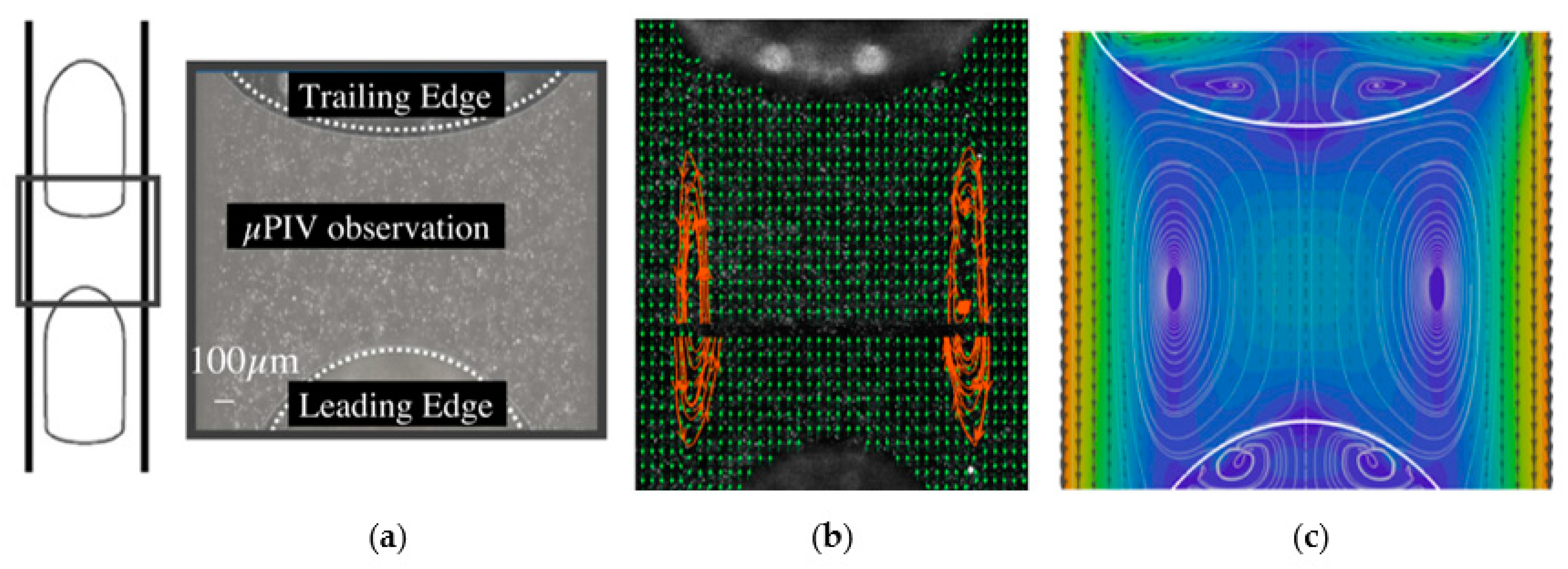
| Using particle image velocimetry Recirculation flow pattern with a high degree of mixing Counter-rotating vortices were observed inside the liquid slugs Velocity profile inside the slugs | Circular Square | GL | [37] | |
| Increasing gas superficial velocity led to the development of the slug flow Low liquid superficial velocity made longer bubbles, shorter liquid slugs profile Slug and annular patterns At high liquid superficial velocity, churn flow was established | Circular Semi-Triangular | GL | [68] | |
| Five flow regimes were observed including bubbly, wedging, slug, bubbly, and dry flow for moderate void fraction The classification of patterns regarding liquid fraction The effect of a sharp return of the channel Void fraction measurement The gravitational effects were taken into account for a bubbly pattern with a spherical gas bubble Liquid droplets may be observable on the walls in wedging pattern | Square | GL | [72] | |
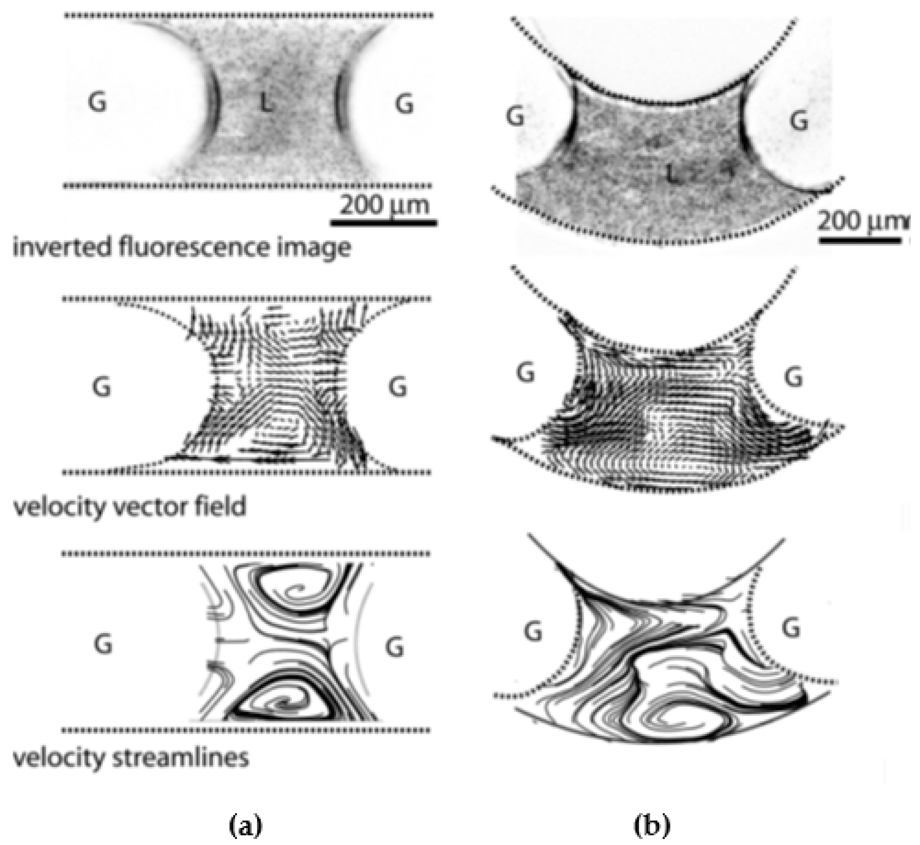
| Using μ-PIV and fluorescent microscopy imaging The liquid phase segments were attached at the corners of the cross-section Gas phase flow improved the mixing and the residence time features | Rectangular | GL | [73] | |
| The hemispherical ends of gas bubbles were not maintained as the Ca increases The nose and the tail of the bubble elongated and flattened as the Re increased The Marangoni effect was observed in experiment efforts and was not taken into account in the numerical simulations | Circular | GL | [44] | |
| Surface modifications Contact angle measurements Meandering microchannel When the length of the bubble was equal to the channel diameter, the flow map was annular At low void fraction when the surface energy was low, the isolated symmetric bubble patterns were observed At moderate void fractions, the flow pattern was asymmetric | Square | GL | [100] | |
| Discussed in the text | Rectangular | LL | [82] | |
| An increase in Ca changes the droplet profile Development of droplet formation with the increase in Ca The significant deviation between the measured film thickness and the Bretherton and Taylor predictions | Circular | LL | [45] | |
| At relatively low flow rates, the slug pattern was established with the length equal to the inner diameter of the tube At high volumetric flow rate, the deformed interface regime was made with long water slugs and small cyclohexane droplets | Circular | LL | [101,102] | |
| Using a μ-PIV technique to capture bubble formation in a T-junction About 25% of the liquid phase passed the gas bubble The gas bubble formation process was included in three steps: Gas bubble growing until occupied the junction Gas bubble developing was decreased as the liquid phase passes the bubbles and the bubble neck was tightened Gas bubble neck was rapidly decreased until approached one-quarter of the diameter before breaking up | Square | GL | [103] | |
| An empirical correlation for a transition from Taylor to unstable slug flow regimes At lower superficial velocities, the Taylor regime was established At higher superficial velocities, the Taylor flow was transited into the dripping flow pattern | Circular | GL | [74,76] | |
| Boiling heat transfer of Fluorinert FC-77 As the heat flux enhanced, the bubble generation rate increased along with an increase of bubble length At moderate heat flux, flow pattern went back and forth between churn and wispy-annular flow regimes | Rectangular | GL (single phase) | [104] | |
| Bubbly flow regime was found at a low gas superficial velocity and a high liquid superficial velocity An increase in gas superficial velocity generated slug regime, where the gas-bubble length was longer than the diameter High liquid velocity and moderated gas superficial velocity produced churn flow map Low liquid superficial velocity and high gas superficial velocity transited the churn to the slug-annular | Circular | GL | [105] | |
| PIV measurements were taken into account Backflow around the liquid slugs were observed The liquid slugs moved faster than that of average flow due to the lubricating effects | Circular | LL | [106] | |
| Using a µ-PIV technique to capture flow structure Slug or Taylor pattern was observed for low superficial velocities As the superficial velocities increased, the lengths of bubbles, and slugs became more variable At high enough gas velocity, the gas phase penetrates the liquid and the length of slugs became shorter | Circular | GL | [107] | |
| Using a laser signal system to provide flow pattern images The channel diameter affects the flow pattern and transition conditions In the bubbly flow regime, the size of the bubbles was approximately was the same as channel diameter | Circular | GL | [108] | |
| A model of mass and momentum balance Stratified flow regime was observed for low oil to gas superficial velocity ratios An increase in the velocity of the gas phase makes the interface to be wavy | Circular | GL | [109] | |
| The number of small bubbles in liquid plug/slug was significantly increased with increasing Vg The size of small bubbles was decreased with increasing Vg or increasing Vl Increasing Vg or decreasing Vl slightly increased the depth of the plug/slug bubble Increasing pipe size enhanced the contribution from large bubbles to a total void fraction Large bubble was accelerated due to small bubble coalescence as flow developed, leading to α decreases | Circular | GL | [96] | |
| Indicating of wave growth and coalescence during slug flow formation For low superficial velocities, the flow pattern remained stratified smooth By an increase of superficial gas velocity, the flow pattern was changed to wavy | Circular | GL | [79] | |
| Comment(s) | Cross-Section | Phases | Reference |
|---|---|---|---|
| The film thickness at the advance of the rear meniscus oscillated The front and rear menisci were slightly different in curvatures Equilibrium bubble profile under surface tension and gravitational effects in a vertical tube | Circular | GL | [30] |
| The film thickness The profiles of front and rear film thickness The film thickness for very elongated gas bubbles | Circular and Square | GL | [35] |
| Bubble profile Flow fields around and between bubbles The motion of a bubble | Square | GL | [145] |
| The influence of velocity on the mass transport phenomenon The effects of liquid slug lengths on flow parameters | Circular | GL | [146] |
| Stronger recirculating flow region as the Ca decreased A liquid backflow was appeared at non-dimensional liquid thickness less than 1/3 Single stagnation point at the vertex of bubble curvature for no-recirculating flow conditions A decrease in the Ca made recirculating flow and moved the stagnation point further the vertex | Parallel plates and Circular | GL | [36] |
| The effects of flow rates on the interface curvature The influence of Eo and wall adhesion on the interface curvature | Circular | Two-phase (parametric) | [147] |
| The rear profile of bubble meniscus versus Ca and Re The effect of Re on the free surface undulations Gas bubble profile The curvature of the gas bubble | Circular | GL | [38] |
| The flow inertia effect was more significant even for deformable wall channels Flexible wall channels were more sensitive than rigid wall channels to the propagation of air bubbles into the walls at low Re and Re/Ca situations The pressure gradient in faraway positions of the tip of the air bubble was generated by Poiseuille flow | 2D | GL | [43] |
| The propagation of liquid plug The adsorption/desorption process of the surfactant was modeled The Marangoni stress results in nearly zero surface velocity at the front meniscus | 2D | GL | [148] |
| Refer to Table 5 | Circular | GL | [44] |
| Slug flow development with time Either uniform or parabolic inlet velocity profile made the same-sized slugs The inlet mixing level influence on the slug lengths | 2D | GL | [58] |
| Bubble shape in slug flow regime The effects of pressure gradient on the bubble profile The presence of gas bubbles made the circulating regions stronger causing a higher momentum transport | 2D | GL | [139] |
| Curved vertical microchannel Slug flow development with time The gas bubbles moved faster than liquid slugs The impact of inlet geometry on the slug development | Circular | GL | [153] |
| The VoF and level-set methods The lack of enough adhesion on wall deformed the rear interface of the slugs | 2D | LL | [106] |
| The VoF method Bubble shapes and formation The effects of superficial velocities on the bubble profiles The influence of nozzle diameter on the bubble formation and shapes | 2D and 3D | GL | [154] |
| Structured-square grid minimizes inaccuracies in the surface tension calculation The process of bubble formation was happened periodically | 2D | GL | [155] |
| The VoF and level set techniques Two commercial simulating software; Ansys and TransAT Bubble formation and development The effect of mixture velocity on the flow pattern and the bubble shapes | 2D | GL | [156] |
| Bubble curvature in slug flow The characteristics of flow were dominantly determined by adherent liquid film thickness An optimized model to minimize the pressure drop and maximize the heat transfer rate | 2D | GL | [26] |
| Comment(s) | Criterion | Mechanism | Cross-Section | Phases | Reference |
|---|---|---|---|---|---|
| Bubbly to slug transition The collision frequency was so low when the void fraction was smaller than 10% The collision frequency was rapidly increased at a void fraction above 25% so that transition to slug flow was rapid even in a strongly liquid | When the rate of coalescence was much more than that of break-up and at a void fraction of 0.25 − 0.3 | Bubble coalescence and void fraction | Circular | GL | [168] |
| Churn to annular happens at a value of | Minimum gas and liquid superficial velocities | Circular | GL | [92] | |
| Slug to slug-bubbly transition No stratified flow pattern was observed in channels with diameter less than 1 mm (it was also verified by [67]) | where, | The production of Re and the We numbers | Rectangular | GL | [64] |
| The churn to annular transition occurred at lower in comparison to the flow reversal transition | the same as [92] | The same as [92] | Circular | GL | [66] |
| Bubbly to slug transition | 0.25 | Void fraction | Circular | GL | [163] |
| The transition from stratified to slug regimes | Kelvin-Helmholtz instability and critical Bond number | Circular | GL | [164] | |
| Upward and vertical flow For several transitions The flowing quality was more suitable than the thermal equilibrium quality to correlate the flow-regime transitions | For bubbly to slug: ~0.3 | Void fraction | Circular | GL | [169] |
| Concentric and eccentric annuli (eccentricity 50%) Upward and vertical flow Mathematical modeling Insignificant effect of eccentricity on transitions for many transitions | and | Probability Density Function (PDF) | Circular | GL | [170] |
| The dominant surface tension in stratified flow regime | Linear stability analysis | Circular | GL | [171] | |
| Bubble to slug transition Upward and vertical flow Turbulence-dependent rate processes controlled the transition at a high flow rate | Average void fraction | Circular | GL | [172] | |
| Discussed in the text | Suratman number | Circular | GL | [65] | |
| Bubble to slug transition Upward and vertical flow | (N/A) | Void fraction | Circular | GL | [173] |
| Bubbly to slug transition The formulation of interfacial transport equations The classification of bubble interactions The categorization of basic mechanisms of bubble coalescence and breakup | (N/A) | Interfacial area concentrations | Circular | GL | [174] |
| Upward and vertical flow for a bubble to slug transition | for for for | Void fraction | Rectangular | GL | [175] |
| Discussed in the text | Discussed in the text | Liquid fraction | Square | GL | [72,100] |
| The bubble size distribution played a crucial role in the flow regime transition and flow patterns | (N/A) | Population Balance Model (PBM) | Circular | GL | [176] |
| Slug into parallel transition happened at small flow rates and large superficial flow ratio By increasing the flow rate, the chaotic flow was changed into annular Equivalent radius was correlated to the We numbers and holdup fraction | Specific range of We for each flow pattern | Weber number | Rectangular | LL | [82] |
| Slug to deformed interface occurred for Slug to drop transition happened in the | Volumetric flow rate ratio | Circular | LL | [45] | |
| Bubbly to slug transition Vertical and upward configuration Effect of bubble size and diameter on the transition | Maximum bubble size | PBM | Circular | LL | [101] |
| Bubbly to slug transition The influence of the bubble population at the inlet region on the regime transition An increase in bubble diameter transits the flow map from bubbly to slug A decrease in tube diameter changed the flow patterns from slug to bubbly regimes | Bubble diameter | PBM | Circular | GL | [177,178] |
| Stable slug regime in the square duct at Stable slug regime in the circular duct at Stable slug regime in the rectangular duct at Stable slug regime in the trapezoidal duct at Annular flow regime at | Reynolds number of gas phase | Square and Trapezoidal | GL | [77] | |
| Slug to churn transition and flow map identification | Void fraction | Circular | GL | [179] | |
| A transition on the slug producing from squeezing to dripping occurred at the junction | Gas volumetric flow rate | Rectangular | GL | [180] | |
| Above the transition value of Ca, an elliptic or oval cross-section area of the gas bubble was observed, and viscous shear overcame the interfacial tension | 0.01 | Capillary number | Quasi-trapezoidal | GL | [80] |
| Correlation | Comment(s) | Flow Parameter | Cross-Section | Phases | Method | Reference |
|---|---|---|---|---|---|---|
| The gas and liquid slug lengths versus dimensionless numbers The effect of gas superficial velocity on slug lengths | Circular | GL | Experimental | [185] | ||
| The slug length was extensively depended on physical means of the experiment, operational conditions, and delivering system | Circular | GL | Experimental | [186] | ||
| The squeezing mechanism affected the size of droplets or bubbles | Rectangular | LL GL | Experimental | [187] | ||
| A decrease in superficial liquid velocity increased the gas slug length An increase in superficial gas velocity enhanced the gas slug length Both slug lengths were moderately affected by the surface tension and wall surface adhesion The gravitational effects on the slug lengths can be ignored | 2D and Circular | GL | Numerical | [58] | ||
| The effects of wettability and the shape of the interface as the volumetric flow rates ratio on the plug length The equilibrium of the shear force and interfacial tension in the form of Ca on the plug length | Square | GL | Experimental | [59] | ||
| An increase in superficial velocities enhanced the slug length Larger bend diameter of the meandering channel made longer slugs | Rectangular | GL | Experimental and Numerical | [60] | ||
| The inlet conditions affect the bubble length significantly The lengths were computed at the centerline of the channel | 2D | GL | Numerical | [155] | ||
and at : | Droplet size at the junction The dependency of droplet diameter on the channel width was insignificant at large width to height ratio | Rectangular | LL | Experimental | [61] | |
| Variation of slug length with volumetric gas and liquid flow rates | Square | GL | Experimental | [188] | ||
| The effects of flow rates on the slug lengths | Rectangular | GL | Experimental | [189] | ||
| The slug lengths of dispersed and continuous phases The slug formation process was not affected by pressure fluctuations Varying slug lengths | Rectangular | LL | Experimental | [190] | ||
| The length of dispersed slugs The effects of operational conditions on the slug lengths The influence of slug velocity and flow rate on the slug length | Circular | LL | Experimental | [191] | ||
| A slug flow in superhydrophobic microchannel An increase in gas flow rate decreased the slug length | Rectangular | GL | Experimental | [180] |
| Correlation | Comment(s) | Flow Parameter | Cross-Section | Phases | Method | Reference |
|---|---|---|---|---|---|---|
| Across a bubble | Dynamic pressure component was dominantly greater than the static value (lubrication approximation) for small Ca The main pressure drop caused by a slight difference between the head and rear curvatures of the bubble | Circular | GL | Experimental and Analytical | [30] | |
| The end effect (K) of the bubble was shown by a constant value of 45 for a function of the Re of for | Circular | GL | Experimental | [64] | ||
| For circular tube: For Square tube: axisymmetric bubbles, non-axisymmetric bubbles, | Matched Asymptotic Analysis Infinite bubbles, Finite bubbles, | Circular and Square | GL | Numerical and Analytical | [35] | |
| An entry region friction model | (N/A) | Circular | GL | Numerical and Analytical | [39] | |
| In uniform film thickness region: | Bubble profiles For axisymmetric bubbles, For bubbles moved faster than liquid and complete by-pass was realized For bubbles moved slower than liquid and reverse flow occurred For bubbles traveled as the same velocity as the liquid and no stagnation pressure | Square | GL | Numerical and Analytical | [145] | |
| The pressure drop of two-phase flow was greater than single-phase flow The Lockhart and Martinelli model did not adequately predict the pressure drop for the laminar flow regime [193] The viscosity of the liquid phase had a key role in the frictional part of the pressure loss | Square | GL | Experimental | [72] | ||
| Pressure drop over the slugs | Circular and Square | GL | Experimental and Numerical | [44,53] | ||
| A decrease in the channel curve radius enhanced the pressure drop An increase in vorticity enhanced the pressure linearly Pressure drop was decreased with | Rectangular | GL | Experimental and Numerical | [60,183] | ||
| The pressure distribution in liquid slug and gas bubble was significantly different due to the interfacial effects The interfacial pressure difference at the nose was greater than the tail of the gas bubble | 2D | GL | Numerical | [152] | ||
| Total pressure drop Curve fitting after scaled using | The pressure drop behavior with was approximated by two asymptotes The total pressure drop was a summation of Poiseuille flow and Taylor components Poiseuille flow was dominant when was greater than 0.1 and Taylor flow was dominant for less than 0.1 | Circular | GL | Experimental | [54] | |
| Shorter liquid slugs and higher inertia force empowered the inner recirculation region At , and Re=200, the pressure drop approached to that proposed by Kreutzer et al. [44] | Square | GL | Experimental | [184] | ||
| Pressure drop was assumed as a summation of frictional and interfacial components The accuracy of the proposed pressure drop model increased for Re greater than 150 | Circular | GL | Experimental | [55] | ||
| Pressure drop was assumed as a summation of frictional and interfacial components Stagnant film (sf) reduced the channel diameter effectively Moving film (mf) considered the dispersed phase frictional drop | Circular | LL | Experimental | [56] | ||
| The dominant role of the number of bubbles compared the gas holdup on the pressure losses | Circular | GL and LL | Analytical and Experimental | [183] | ||
| The pressure drop prediction was only valid for long droplets The interfacial pressure drop increased as the diameter decreases The interfacial pressure drop was negligible for very long slugs and droplets | Circular | LL | Experimental and Numerical | [48] | ||
| Total pressure drop was increased as the total volumetric flow rate enhances The total pressure drop approaches to an asymptotic value of 16 for single-phase flow for greater than 0.12 | Circular | GL LL | Experimental | [57] |
Publisher’s Note: MDPI stays neutral with regard to jurisdictional claims in published maps and institutional affiliations. |
© 2021 by the authors. Licensee MDPI, Basel, Switzerland. This article is an open access article distributed under the terms and conditions of the Creative Commons Attribution (CC BY) license (https://creativecommons.org/licenses/by/4.0/).
Share and Cite
Etminan, A.; Muzychka, Y.S.; Pope, K. A Review on the Hydrodynamics of Taylor Flow in Microchannels: Experimental and Computational Studies. Processes 2021, 9, 870. https://doi.org/10.3390/pr9050870
Etminan A, Muzychka YS, Pope K. A Review on the Hydrodynamics of Taylor Flow in Microchannels: Experimental and Computational Studies. Processes. 2021; 9(5):870. https://doi.org/10.3390/pr9050870
Chicago/Turabian StyleEtminan, Amin, Yuri S. Muzychka, and Kevin Pope. 2021. "A Review on the Hydrodynamics of Taylor Flow in Microchannels: Experimental and Computational Studies" Processes 9, no. 5: 870. https://doi.org/10.3390/pr9050870