
Computational Modeling of Flow Characteristics in Three Products Hydrocyclone Screen


Abstract
:1. Introduction
2. Methodology
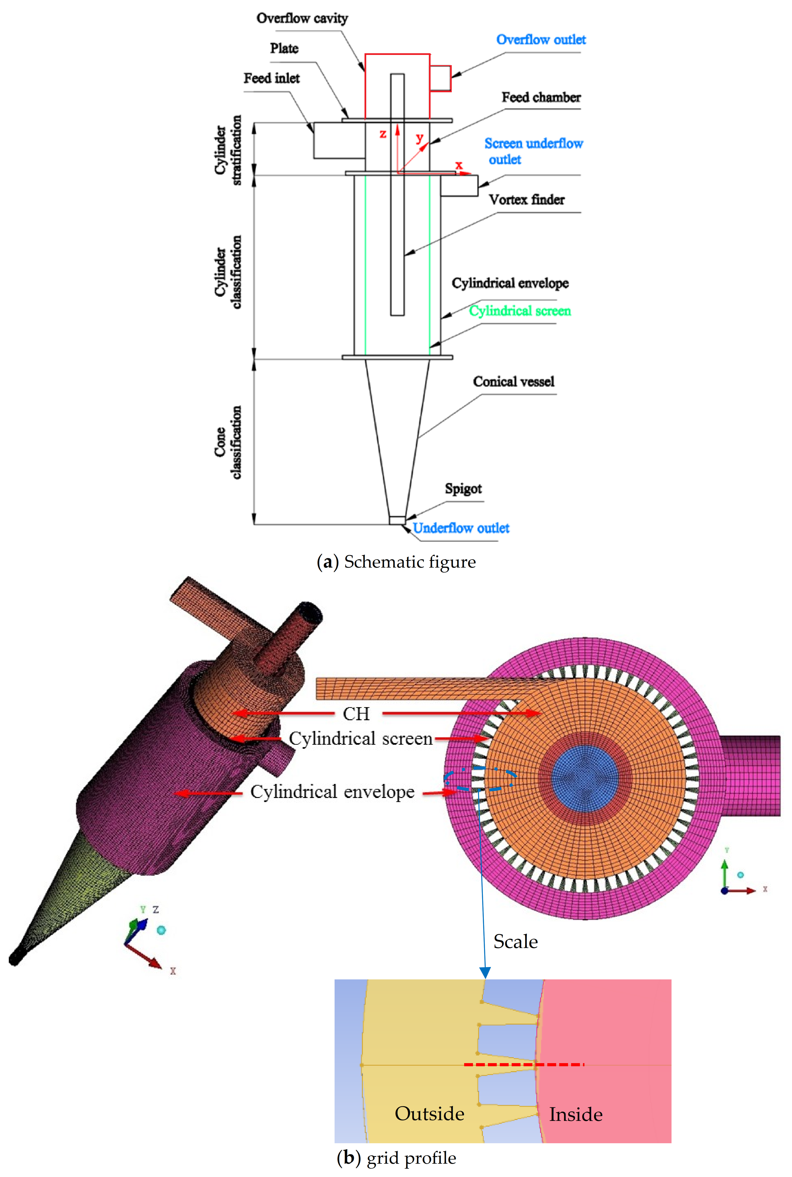
2.1. Geometric Models
2.2. Numerical Models
2.3. Boundary Conditions and Initialization
3. Results and Discussions
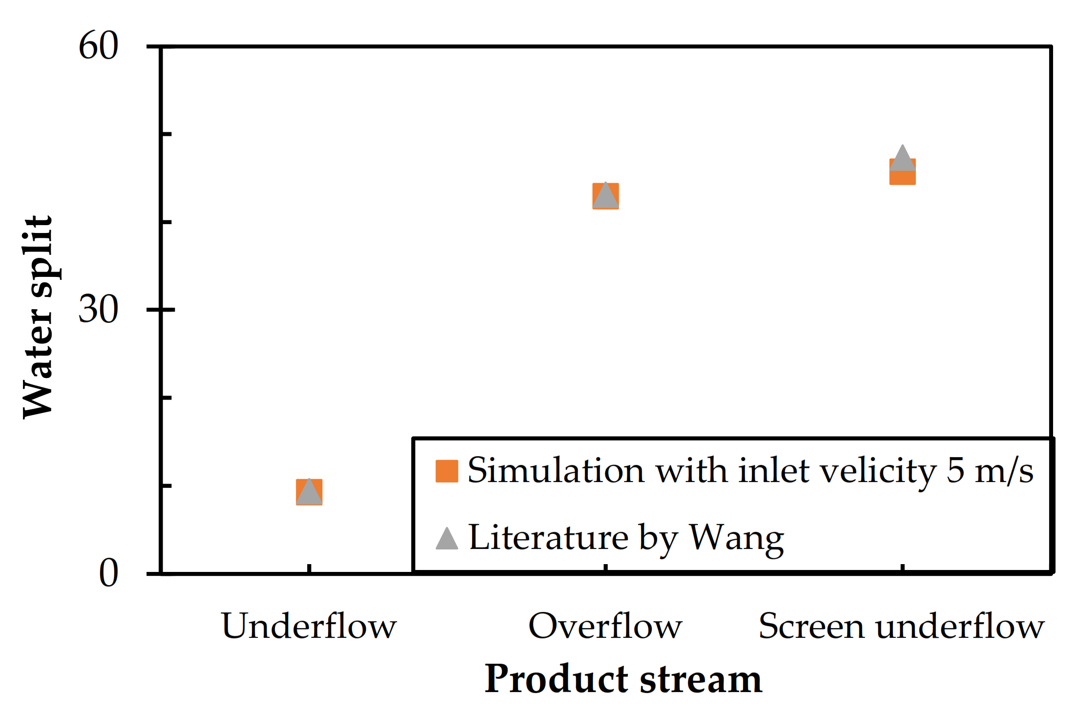
3.1. Validation
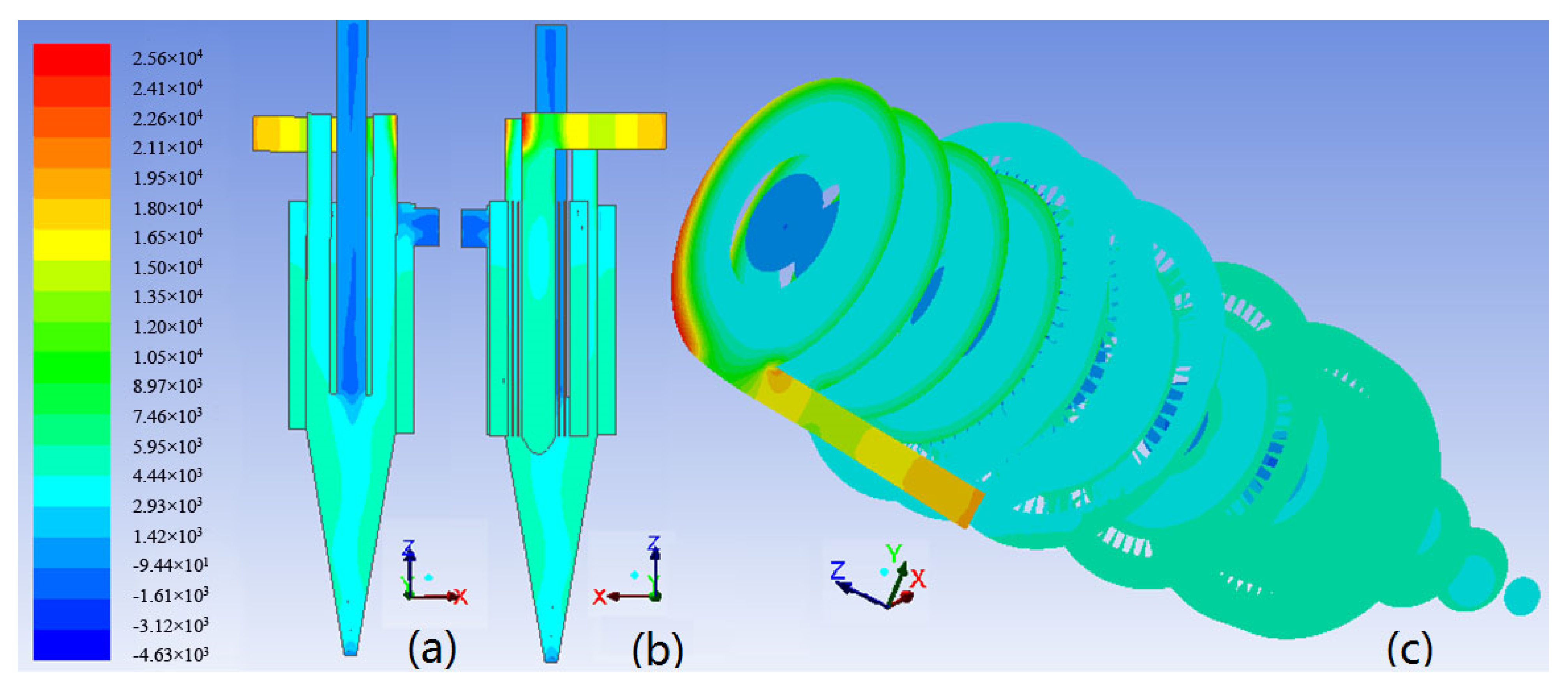
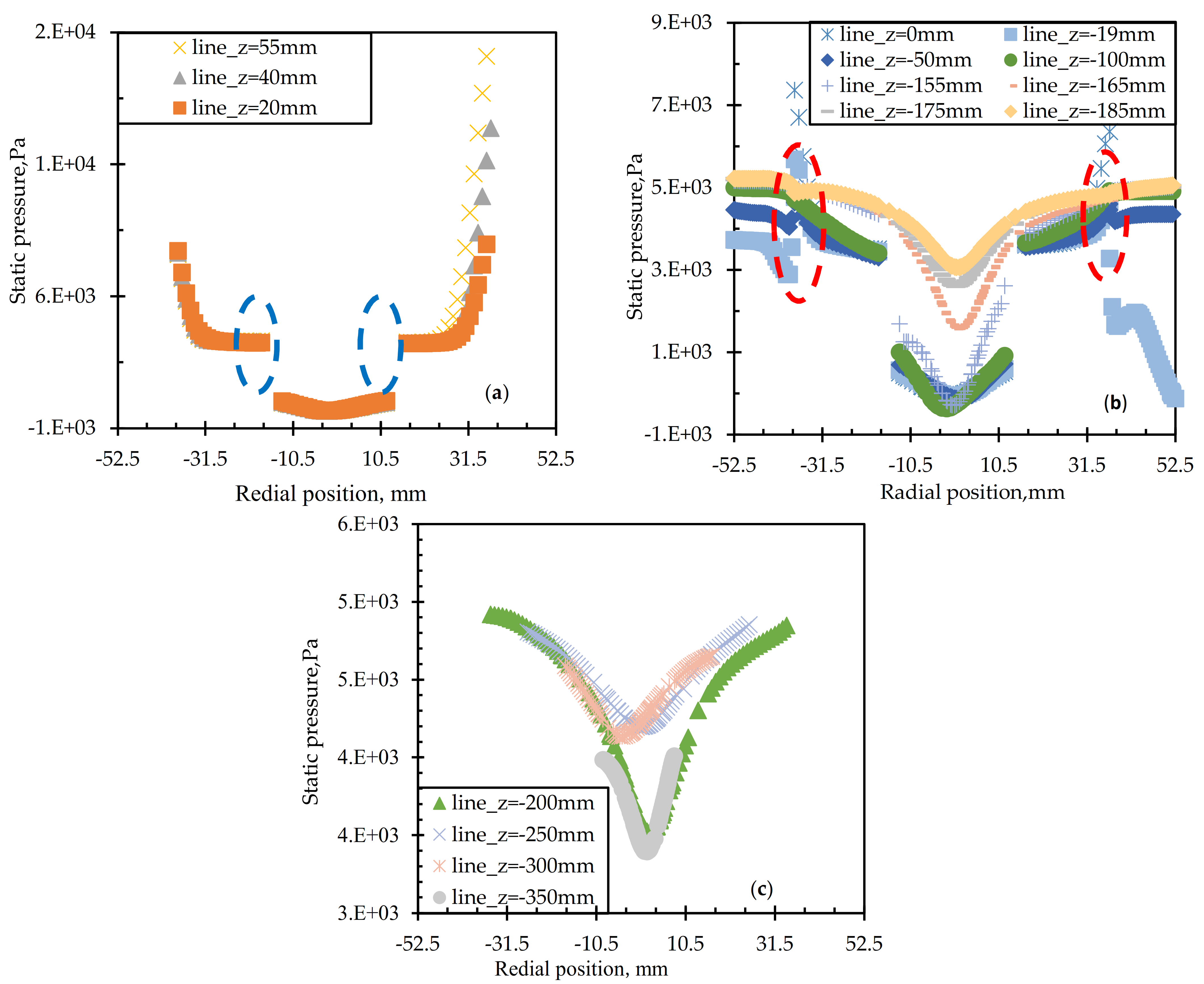
3.2. Pressure Distribution
3.3. Turbulence Feature
4. Conclusions
- (1)
- Generally, the distribution of static pressure was axisymmetric, and its value decreased with the increase in the axial depth. The maximum was located near the tangential inflection point of the feed inlet, while the minimum appeared in each outlet. However, due to the left tangential inlet and the right screen underflow outlet, local asymmetry can be observed.
- (2)
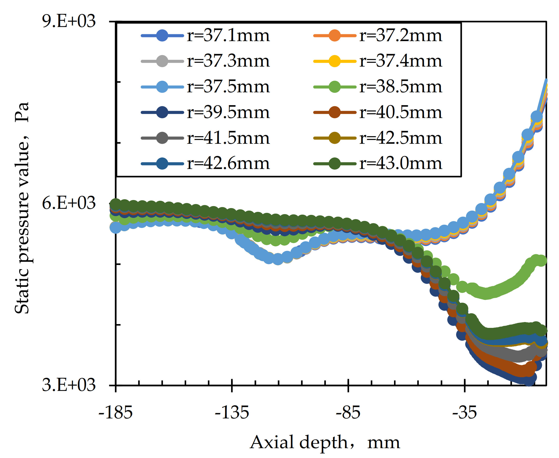
- In the same horizontal plane, the static pressure decreased gradually along the wall to the center. Near the cylindrical screen, as the axial depth increased, the static pressure inside the cylindrical screen gradually decreased, while that outside the cylindrical screen regularly increased. As the axial depth increased to about −85 mm, the static pressure of the two sides was closely in equilibrium. Then, the pressure on the outside of the screen became higher than that on the inside of the screen.
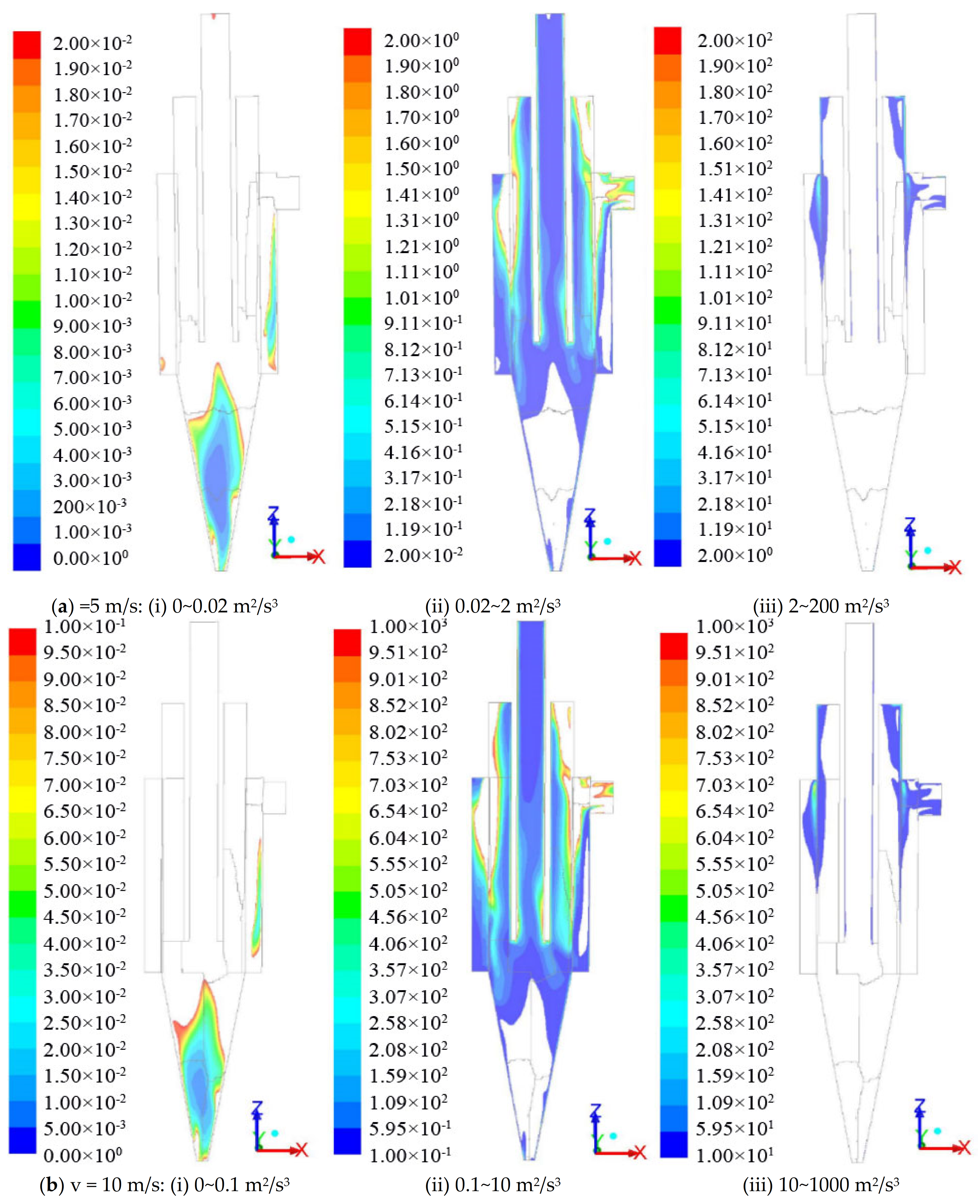
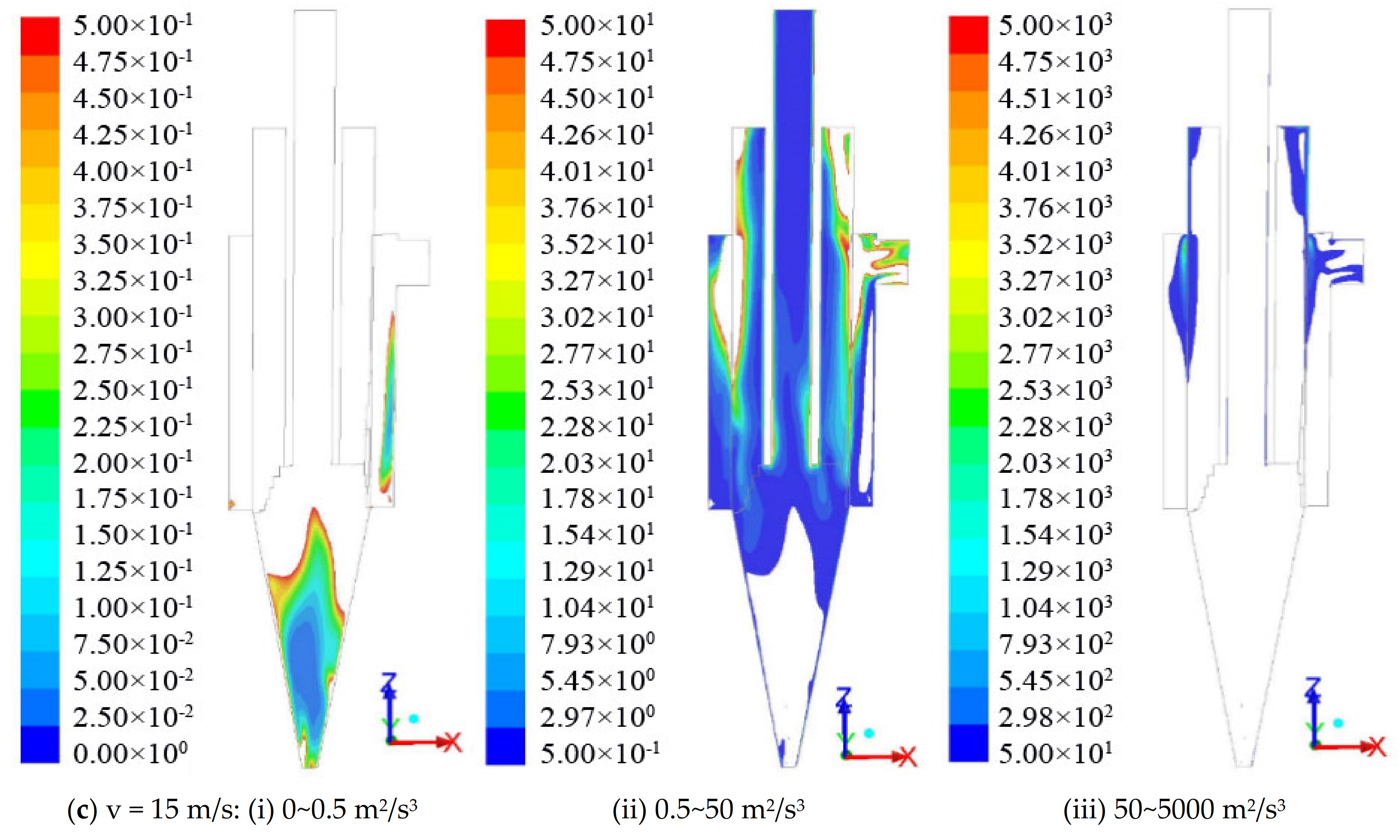
- (3)
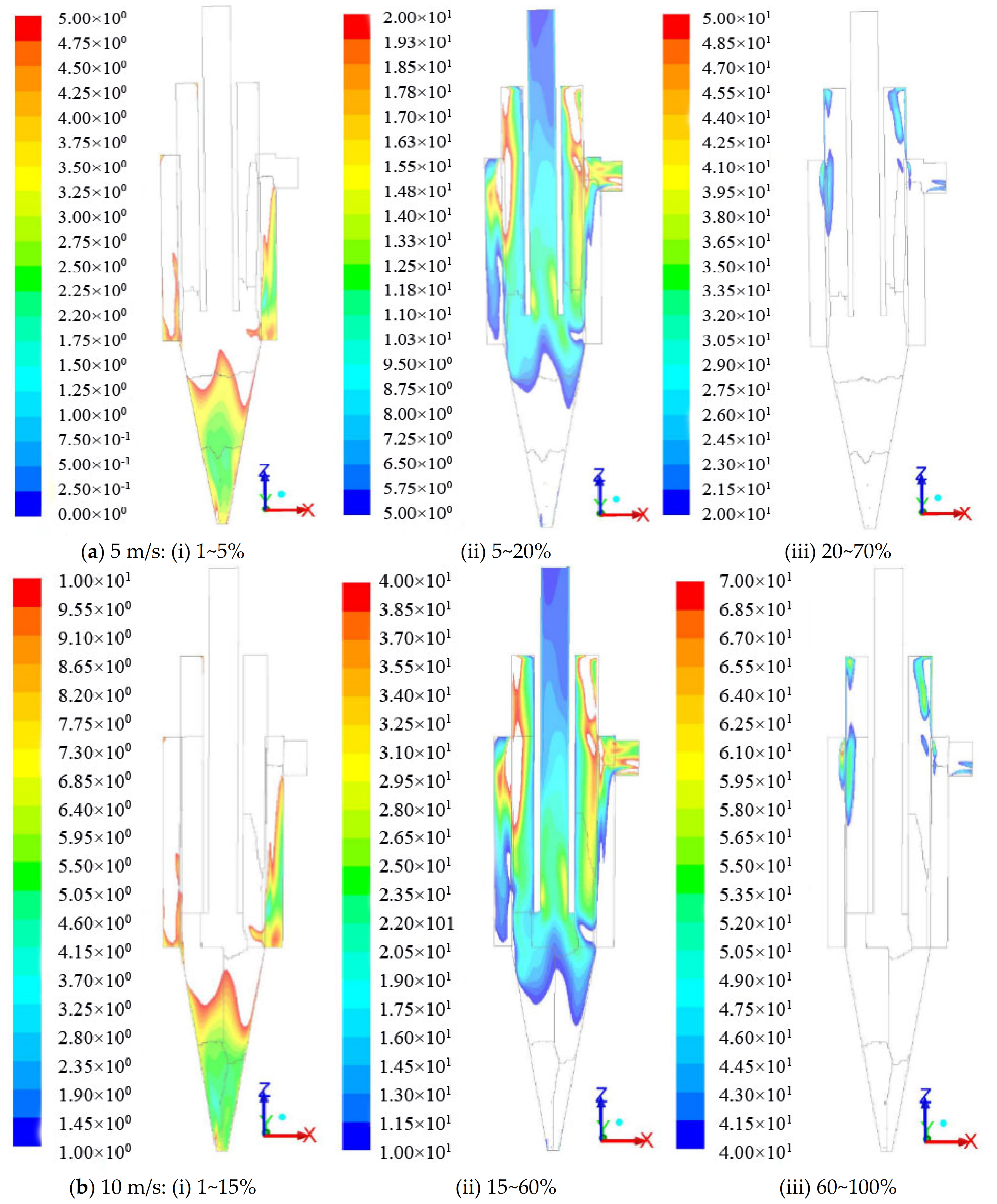
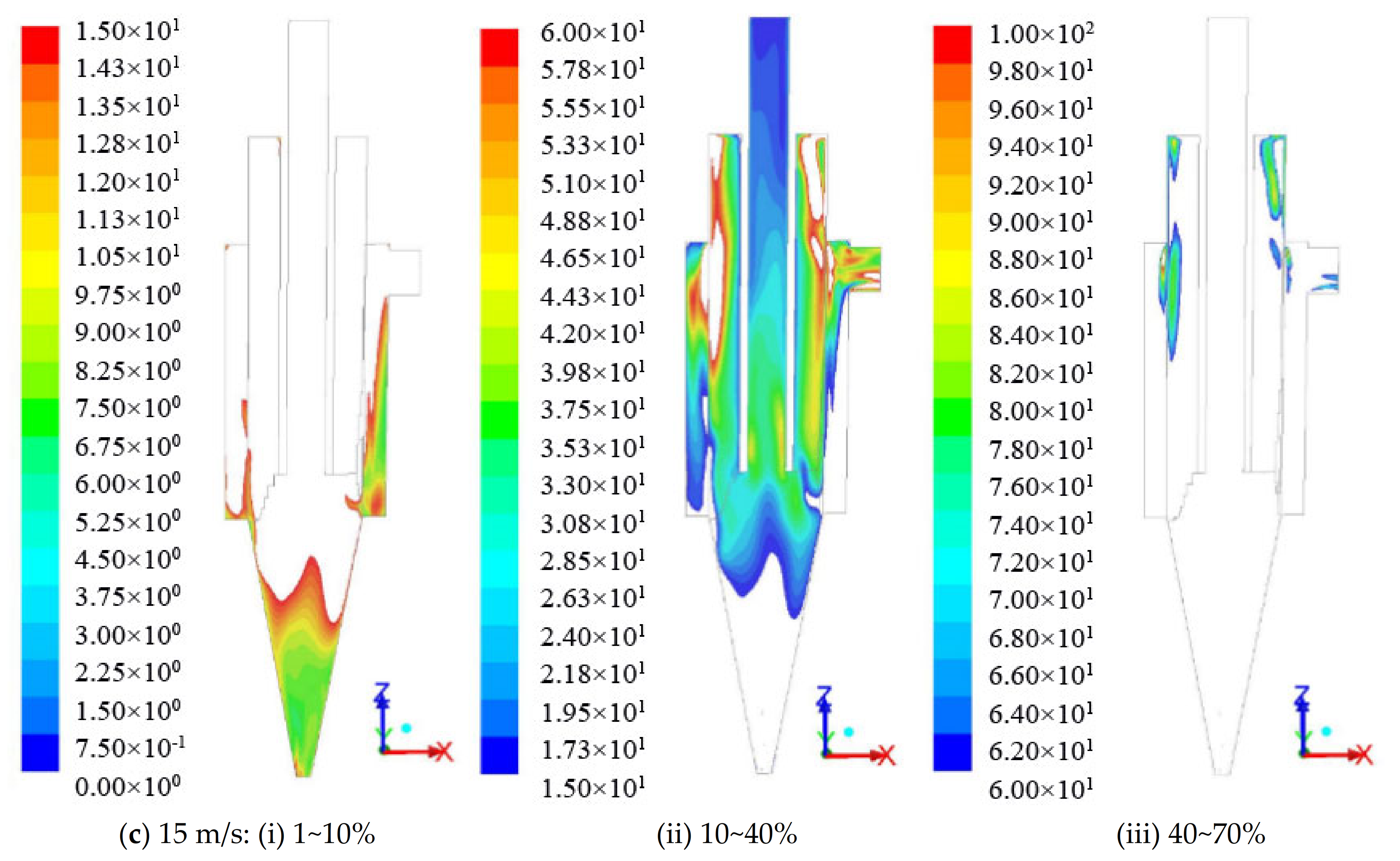
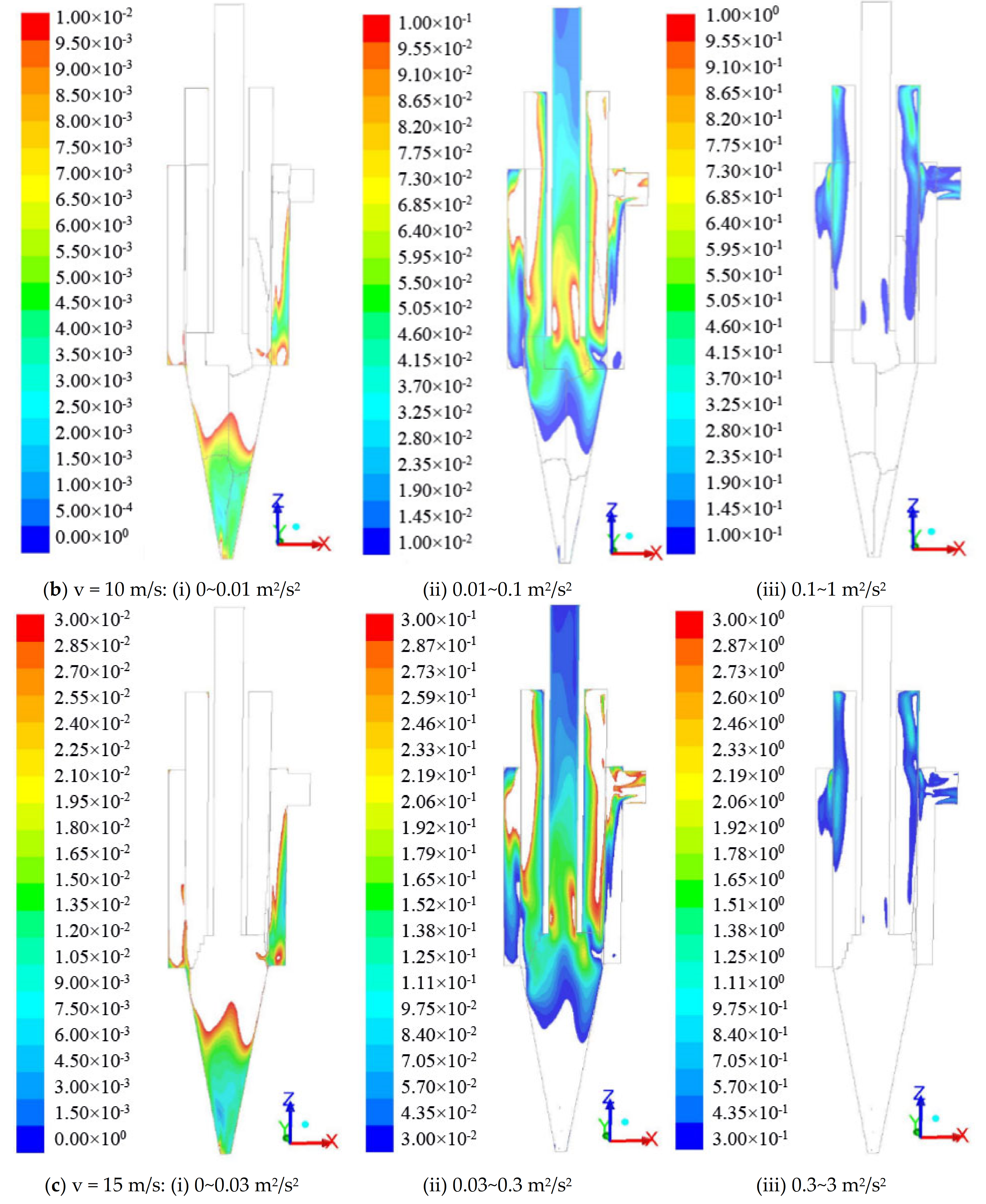
- The turbulence intensity I, turbulence kinetic energy k, and turbulence dissipation rate ε of the fluid flow in TPHS exhibit similar distributions; that is, the values decreased with the increase in axial depth. Meanwhile, from high to low, the pressure values are distributed in the feed chamber, the cylindrical screen, and the conical vessel; the value inside the screen was higher than the outer value.
Author Contributions
Funding
Institutional Review Board Statement
Informed Consent Statement
Data Availability Statement
Conflicts of Interest
Nomenclature
| Velocity vector (m/s) | |
| Mean velocity component (m/s) | |
| Fluctuation velocity component (m/s) | |
| , | x, y, or z components |
| , | Phase in fluid |
| () | The mass transfer from phase () to phase () |
| turbulence kinetic energy at the wall-adjacent cell centroid, P | |
| t | time (s) |
| mean velocity of the fluid at the wall-adjacent cell centroid, P | |
| , , | position (m) |
| distance from the centroid of the wall-adjacent cell to the wall, P | |
| Kronecker delta function | |
| density (kg/m3) | |
| wall shear stress |
References
- Wills, B.A.; Napier-Munn, T. Wills’ Mineral Processing Technology: An Introduction to the Practical Aspects of Ore Treatment and Mineral Recovery; Butterworth-Heinemann: London, UK, 2015. [Google Scholar]
- Roldán-Villasana, E.J.; Williams, R.A.; Dyakowski, T. The origin of the fish-hook effect in hydrocyclone separators. Powder Technol. 1993, 77, 243–250. [Google Scholar] [CrossRef]
- Mohanty, M.K.; Palit, A.; Dube, B.J.M.E. A comparative evaluation of new fine particle size separation technologies. Miner. Eng. 2002, 15, 727–736. [Google Scholar] [CrossRef]
- Eckert, K.; Schach, E.; Gerbeth, G.; Rudolph, M. Carrier Flotation: State of the Art and its Potential for the Separation of Fine and Ultrafine Mineral Particles. Mater. Sci. Forum 2019, 959, 125–133. [Google Scholar] [CrossRef]
- Hla, B.; Yl, B.; Fang, G.A.; Zhan, Z.B.; Lx, B.J.C. CFD–DEM simulation of material motion in air-and-screen cleaning device. Comput. Electron. Agric. 2012, 88, 111–119. [Google Scholar]
- Chang, Y.-L.; Ti, W.-Q.; Wang, H.-L.; Zhou, S.-W.; Huang, Y.; Li, J.-P.; Wang, G.-R.; Fu, Q.; Lin, H.-T.; Wu, J.-W. Hydrocyclone used for in-situ sand removal of natural gas-hydrate in the subsea. Fuel 2021, 285, 119075. [Google Scholar] [CrossRef]
- Santana, R.; Farnese, A.; Fortes, M.; Ataide, C.; Barrozo, M. Influence of particle size and reagent dosage on the performance of apatite flotation. Sep. Purif. Technol. 2008, 64, 8–15. [Google Scholar] [CrossRef]
- Vieira, L.; Barrozo, M. Effect of vortex finder diameter on the performance of a novel hydrocyclone separator. Miner. Eng. 2014, 57, 50–56. [Google Scholar] [CrossRef]
- Chu, L.-Y.; Yu, W.; Wang, G.-J.; Zhou, X.-T.; Chen, W.-M.; Dai, G.-Q. Enhancement of hydrocyclone separation performance by eliminating the air core. Chem. Eng. Process. Process. Intensif. 2004, 43, 1441–1448. [Google Scholar] [CrossRef]
- Dueck, J.; Farghaly, M.; Neesse, T. The theoretical partition curve of the hydrocyclone. Miner. Eng. 2014, 62, 25–30. [Google Scholar] [CrossRef]
- Dos Santos, M.A.; Santana, R.C.; Capponi, F.; Ataíde, C.H.; Barrozo, M.A. Effect of ionic species on the performance of apatite flotation. Sep. Purif. Technol. 2010, 76, 15–20. [Google Scholar] [CrossRef]
- Kursun, H.; Ulusoy, U. Influence of shape characteristics of talc mineral on the column flotation behavior. Int. J. Miner. Process. 2006, 78, 262–268. [Google Scholar] [CrossRef]
- Mainza, A.; Narasimha, M.; Powell, M.; Holtham, P.; Brennan, M. Study of flow behaviour in a three-product cyclone using computational fluid dynamics. Miner. Eng. 2006, 19, 1048–1058. [Google Scholar] [CrossRef]
- Wang, C.; Chen, J.; Shen, L.; Ge, L. Study of flow behaviour in a three products hydrocyclone screen: Numerical simulation and experimental validation. Physicochem. Probl. Miner. Process. 2019, 55, 879–895. [Google Scholar]
- Wang, C.; Chen, J.; Shen, L.; Hoque, M.M.; Ge, L.; Evans, G.M. Inclusion of screening to remove fish-hook effect in the three products hydro-cyclone screen (TPHS). Miner. Eng. 2018, 122, 156–164. [Google Scholar] [CrossRef]
- Wang, C.; Yu, A.; Zhu, Z.; Liu, H.; Khan, S. Mechanism of the Absent Air Column in Three Products Hydrocyclone Screen (TPHS): Experiment and Simulation. Processes 2021, 9, 431. [Google Scholar] [CrossRef]
- Hirt, C.; Nichols, B. Volume of fluid (VOF) method for the dynamics of free boundaries. J. Comput. Phys. 1981, 39, 201–225. [Google Scholar] [CrossRef]
- Gibson, M.M.; Launder, B. Ground effects on pressure fluctuations in the atmospheric boundary layer. J. Fluid Mech. 1978, 86, 491–511. [Google Scholar] [CrossRef]
- Launder, B.; Reece, G.J.; Rodi, W. Progress in the development of a Reynolds-stress turbulence closure. J. Fluid Mech. 1975, 68, 537–566. [Google Scholar] [CrossRef] [Green Version]
- Launder, B.E. Second-moment closure: Present … and future? Int. J. Heat Fluid Flow 1989, 10, 282–300. [Google Scholar] [CrossRef]
- Shah, H.; Majumder, A.; Barnwal, J. Development of water split model for a 76mm hydrocyclone. Miner. Eng. 2006, 19, 102–104. [Google Scholar] [CrossRef]
- Vakamalla, T.R.; Kumbhar, K.S.; Gujjula, R.; Mangadoddy, N. Computational and experimental study of the effect of inclination on hydrocyclone performance. Sep. Purif. Technol. 2014, 138, 104–117. [Google Scholar] [CrossRef]


| Items | Size | Items | Size |
|---|---|---|---|
| Inner diameter of screen mesh | 75 mm | Height of cylindrical envelope | 185 mm |
| Size of aperture | 0.65 mm | Inner diameter of column | 75 mm |
| Thickness of screen bar | 5 mm | Inner diameter of vortex finder | 25 mm |
| Width of screen bar | 3.25 mm | Height of cylindrical envelope | 185 mm |
| Height of screen mesh | 185 mm | Inner diameter of screen underflow outlet | 30 mm |
| Size of feed inlet (length × width) | 29 mm × 8 mm | Angle of cone section | 20° |
| Length of feed cavity | 70 mm | Inner diameter of underflow outlet | 10 mm |
Publisher’s Note: MDPI stays neutral with regard to jurisdictional claims in published maps and institutional affiliations. |
© 2021 by the authors. Licensee MDPI, Basel, Switzerland. This article is an open access article distributed under the terms and conditions of the Creative Commons Attribution (CC BY) license (https://creativecommons.org/licenses/by/4.0/).
Share and Cite
Yu, A.; Wang, C.; Liu, H.; Khan, M.S. Computational Modeling of Flow Characteristics in Three Products Hydrocyclone Screen. Processes 2021, 9, 1295. https://doi.org/10.3390/pr9081295
Yu A, Wang C, Liu H, Khan MS. Computational Modeling of Flow Characteristics in Three Products Hydrocyclone Screen. Processes. 2021; 9(8):1295. https://doi.org/10.3390/pr9081295
Chicago/Turabian StyleYu, Anghong, Chuanzhen Wang, Haizeng Liu, and Md. Shakhaoath Khan. 2021. "Computational Modeling of Flow Characteristics in Three Products Hydrocyclone Screen" Processes 9, no. 8: 1295. https://doi.org/10.3390/pr9081295