Abstract
A novel delay-dependent stability criterion for Takagi-Sugeno (T-S) fuzzy systems with multiplicative noise is addressed in this paper subject to passivity performance. The general case of interval time-varying delay is considered for the practical control issue. For the criterion, an integral Lyapunov-Krasovskii function is proposed to derive some sufficient relaxed conditions and to avoid the derivative of the membership function. Moreover, a free-matrix inequality is adopted to deal with the delay terms such that the available derivative of time-varying delay is bigger than one. In order to employ a convex optimization algorithm to find the control gain, a projection lemma is applied to acquire the Linear Matrix Inequality (LMI) form of the sufficient conditions. With the obtained gains, a fuzzy controller is designed by the concept of Parallel Distributed Compensation (PDC) such that the delayed T-S fuzzy systems with multiplicative noise are asymptotically stable and passive in the mean square. Finally, a stabilization problem of the ship’s autopilot dynamic system and some comparisons are discussed during the simulation results.
1. Introduction
To simplify stability problems of nonlinear systems, the Takagi-Sugeno (T-S) fuzzy system [1,2,3,4,5,6,7,8,9,10,11,12,13,14,15,16,17] is generally widely used by merging a group of linear systems and membership functions. Furthermore, a concept of Parallel Distributed Compensation (PDC) was first proposed by [1] to design a fuzzy controller whose structure is the same as the T-S fuzzy system. Based on the T-S fuzzy system and PDC concept, many linear stability theories can be directly adopted to discuss the control issues of nonlinear systems. Moreover, some stability criteria [2,3,4,5,6,7,8] for nonlinear stochastic systems were developed via the T-S fuzzy system. Referring to [6,7,8], a stochastic differential equation was modeled by combining a deterministic differential equation and a multiplicative noise term. The term consists of states and Brownian motion [8] and is employed to describe stochastic behavior. To discuss the stability of a stochastic system, the Itô formula and concept of mean square are generally required according to the unpredicted property and complete probability. Based on the T-S fuzzy model and stochastic differential equation, several PDC-based fuzzy controller design methods were developed to achieve performances such as the mixed performance [9,10,11], passivity [7,12,13], robustness [5,17], and so on.
Usually, time delay is a common effect that causes poor control performance during the signal transmission of physical systems such as the COVID epidemic, a ship stabilizer, a network system, a chemical changer, and a hydraulic machine [18]. For example, an internal time-varying delay is considered a general case because both upper and lower bounds are simultaneously considered. According to this consideration, the stability of systems with an interval time-varying delay is more difficult and complex to achieve compared to the stability of systems with other delay cases [19,20]. Furthermore, some delay-dependent stability criteria [21,22,23,24] were discussed by the Lyapunov-Krasovskii function. Based on the T-S fuzzy modeling approach, delay-dependent stability criteria [25,26] have been developed for nonlinear systems. The Lyapunov-Krasovskii function used by [25,26] is constructed by a common positive definite matrix. It is well known that a common matrix causes conservative results when solving a control problem. To achieve a relaxed criterion, the Lyapunov-Krasovskii function has been improved by choosing a parameter-dependent structure [27] to increase the number of variables. Furthermore, several technologies [28,29] were proposed to introduce some slack variables and relax the conservatism of controller design methods. On the other hand, a limitation is naturally caused such that the derivative of the time-varying function of delays is less than one. Referring to [29], a free-matrix inequality was developed to eliminate the limitation caused by the derivation. Unfortunately, the controller design problem of the delayed nonlinear systems was not discussed by [29] due to the conversion of sufficient conditions for satisfying the form of Linear Matrix Inequality (LMI). Therefore, the relaxed stabilization issue of a nonlinear delayed system is worth investigating for the design of a PDC-based fuzzy controller.
Most of the stability criteria in the present results were proposed by choosing the Lyapunov function. For a polynomial description, such as the T-S fuzzy system [4] and linear parameter varying systems [30], a class of fuzzy Lyapunov functions and parameter-dependent Lyapunov functions were employed to increase the relaxation of the proposed criteria. Referring to [15], although multiple matrices in the fuzzy Lyapunov function provide relaxation, a potential conservatism is caused by the derivative of the membership function. Hence an integral Lyapunov function was proposed by [16] to avoid the conservatism caused by the derivative. Depending on the structure of the matrices in the integral Lyapunov function, it is hard to convert the sufficient condition into an LMI form. Thus, an extra iterative LMI algorithm [12] was proposed to find a solution to the condition derived by the integral Lyapunov function. It should be noted that the extra algorithm causes not only some conservatism but also computational complexity. Therefore, an interesting solution to applying the integral Lyapunov function is to extend the advantage for other stability criteria without using an extra algorithm.
According to the above motivations, a novel delay-dependent stability criterion of a nonlinear stochastic system is investigated in this paper subject to passivity. Based on the modeling approach and stochastic differential equation, the nonlinear stochastic system is represented by a T-S fuzzy system with multiplicative noise terms. For the general delay effect, the interval time-varying case is considered to discuss the delay-dependent stability problem. For the problem, an integral Lyapunov-Krasovskii function is proposed to avoid the conservatism caused by the derivative of the membership function. Dealing with the delay term in the derivative, the free-matrix inequality is employed such that the differentiation of the delay function is not limited by one. In addition to the delay, the attenuation performance is also concerned by the passivity theory [24] to constrain the effect of external disturbance on the system. With the Itô formula, some sufficient conditions are derived to ensure the asymptotical stability of the system in the mean square. Furthermore, the concept of PDC is adopted to establish a fuzzy controller and to discuss the stabilization problem. Based on the convex optimization algorithm, the projection lemmas [28] are employed such that the derived conditions are in strict LMI form. To summarize the contributions of this paper, three points are provided: (1) A novel integral Lyapunov-Krasovskii function is proposed to eliminate the conservatism caused by the derivative of the membership function. (2) The differentiation of the time-varying function of delay is bigger than the one that increases the application of the proposed design method. (3) No extra algorithm is required to find feasible solutions to the derived conditions.
The paper is organized as follows: In Section 2, the stability problem of the delayed T-S fuzzy system with multiplicative noise is presented. In Section 3, the relaxed stability criterion is proposed to ensure the asymptotical stability of the system in the mean square. The numerical simulation and comparisons are provided in Section 4. Finally, some conclusions to this paper are stated in Section 5.
Notation: denotes the elements with their symmetry matrices. denotes the diagonal matrix with dimension , whose all-diagonal element is . denotes the identity matrix with proper dimension. denotes the transpose matrix. denotes the expected value of .
2. System Descriptions and Problem Statements
The continuous-time T-S stochastic system with interval time-varying delay and external disturbance is presented as follows:
IF is and is and … and is THEN
where is the state vector, is the control input vector, is the disturbance, is the system output, is the initial condition, is a scalar continuous type Brownian motion satisfying the independent increment property [6] such as , and . Besides, , , , , , , , , and are the constant matrices with compatible dimension, is the number of fuzzy rules, is the fuzzy set, is the premise variable number and specifies which -based fuzzy set is used in the i-th fuzzy rule, therefore for any . is the time-varying delay satisfying and . The state equations for the system (1)–(2) can be inferred in terms of rules as follows:
where , , and .
Based on the PDC concept [1], the following fuzzy controller is presented to compensate the considered system (3).
where is the control gain, which needs to be found. The final output of (4) can also be represented as follows:
Substituting (4) into (2), the following closed-loop system can be inferred.
where and . For simplification, is defined as .
For the closed-loop system (6), the concerned stability and attenuation performance are respectively ensured by the following definitions.
Definition 1.
[8] For the closed-loop systems (6), the solution is asymptotically stable in the mean square when and are converged to zero as .
Definition 2.
[8] If the matrices ,
, and exist to satisfy the following inequality, then the system (6) with and is called passive.
where is the terminal time.
Referring to [8], the inequality (7) can be reduced by several performance indexes by choosing different , , and . To deal with the delay terms during the derivative, the following free-matrix inequality is applied.
Lemma 1.
[29] Let be a differentiable function: . For symmetric matrices and , and matrices and , satisfying:
Moreover, the following inequality holds.
where,,,,,and.
Besides, the following projection lemma is applied to transfer the bilinear condition into the LMI problem.
Lemma 2.
[30] Giving the matrices , and which satisfy and , if there exists any matrix such that:
then the following inequalities are held.
and
where and are matrices whose column form is the null-space of and respectively.
Lemma 3.
[24] For the given matrices , and , if there exists then the following inequalities are equivalent:
and
According to [16], the positive matrix of the integral Lyapunov function which has the path-independent property is constructed as follows:
in which, is a positive definite symmetric matrix and defined as follows:
Referring to (16), the off-diagonal elements are the same, but the diagonal elements are different according to the fuzzy sets in the premise parts of the fuzzy rules. Furthermore, the j-th diagonal elements are independent from each other for the different -based fuzzy sets. One can refer to [16] for detailed information on the integral Lyapunov function.
In the next section, a novel delay-dependent stability criterion for the closed-loop system (6) is developed via the integral Lyapunov-Krasovskii function. Furthermore, the above lemmas are applied to reduce the conservatism of the criterion. Based on the criterion, the asymptotical stability and passivity are achieved in the mean square.
3. Stability Criterion Subject to Passivity Constraint
In this section, some sufficient conditions guaranteeing the asymptotical stability of the closed-loop system (6) are derived subject to passivity in the mean square. Through applying Lemmas 2 and 3, some LMI conditions are derived and can be directly solved by a convex optimization algorithm to find feasible solutions. With the obtained solutions, the fuzzy controller (5) can be established to achieve the required performance.
Theorem 1.
Giving the matrices,and,scalars,,andsatisfying the definition of,the closed-loop system (6) is asymptotically stable subject to passivity in the mean square if there exist positive symmetric matrices,,,,,and,symmetrical matrices,,,,,,and,any matrices,,, ,,,,,,andsuch that:
and
where
and
Proof of Theorem 1.
Choosing the following integral Lyapunov-Krasovskii function.
where
and
Through applying the Itô formula, the following derivation of along the trajectories of (6) can be obtained.
and
Combining Equations (23)–(29), one has the following equation, when taking the expectation with the independent increment property
Applying Lemma 1, the following inequalities are inferred from the terms in (24)–(26).
and
where
and
From the results of (31)–(33), the following inequality can be easily found from (30):
where
and
Let us define the following cost function with zero initial condition for all .
where
Substituting (2) and (34) into (36), one has.
Obviously, if the conditions (17)–(21) are satisfied, then one can obtain implying in (37). From (35), one can further infer the following inequalities for all nonzero external disturbances due to .
or
Because (39) is equal to (7), the closed-loop system (6) is passive due to Definition 2. Next, it is necessary to show that the system is asymptotically stable in the mean square with . According to (37), if condition (17) holds, then one has . By assuming , one can find from (36) due to . Since and , one can obtain the following equation from (30).
Obviously, if holds, then is easily inferred by (40). Based on Definition 1, the asymptotical stability of the closed-loop system (6) is ensured in the mean square according to . This proof is completed. □
Remark 1.
According to the existence ofand, the conditions inTheorem 1are not in the standard LMI form with. However, it is the linear function of the variablesfor allandif four cases of,,andare set. It can easily use the convex optimization algorithm for four cases to obtain feasible solutions.
The derived conditions in Theorem 1 belong to a bilinear problem which cannot be directly solved by the convex optimization algorithm. Based on Lemmas 2 and 3, the conditions are transferred into LMI forms in the following theorem.
Theorem 2.
For the given matrices,, and,scalars,,, andsatisfying the definition of, and the scalarsand, the closed-loop system (6) is asymptotically stable and subject to passivity in the mean square if positive definite matrices exist,,,,,and, symmetrical matrices,,,,,,and,and any matrices,,,, ,,,,,,,,,andsuch that:
and
where
and
Proof of Theorem 2.
Without the general lost, condition (41) can be rewritten as follows:
where
and
In this paper, the orthogonal matrices for and are respectively chosen as:
and
Based on Lemma 2, and , the following inequalities are also held form (46).
and
where
and
Furthermore, inequality (47) can be rewritten as follows:
where , , and .
According to Lemma 3 and (49), the following inequality is also hold.
Through the arrangement, one can infer that the inequality (50) is equal to the condition (14). Thus, if condition (41) holds, then condition (17) is also satisfied. Moreover, the closed-loop system (6) is asymptotically stable in the mean square subject to passivity. The proof of Theorem 2 is complete. □
Remark 2.
According toand, the conditions inTheorem 2are not in the strict LMI form. Based onRemark 1, the convex optimization algorithm is employed to find the feasible solutions to simultaneously satisfying four cases. However, that may increase the complexity of the number of conditions. On the other hand, one can find the conservative solutions for conditions in theorems through setting the terms asandinto, andinto, respectively. Although the terms provide conservative solutions, the number of LMIs can be reduced from 4r2 + 4 to r2 + 4 such that the proposed design method is easily used to design the controller (5).
Remark 3.
The parameters andand matrices andare introduced in Theorem 2 based on Lemmas 2 and 3. Moreover, the number of variables in Theorem 2 is 28 + 2r. Although the huge number of variables increases the freedom of searching for feasible solutions, it also brings computational complexity.
Following the description of Remark 2, the relaxed conditions in Theorem 2 with four cases are solved via the convex optimization algorithm for discussing the stabilization problem of the ship’s autopilot system in the following section. Moreover, a comparison is also provided to discuss the conservatism of the proposed stability criterion.
4. Simulation Result
In this section, two cases are provided to demonstrate the effectiveness and applicability of the proposed delay-dependent stability criterion. In Case 1, the stabilization problem of the ship’s autopilot dynamic system [31] is discussed by Theorem 2. In Case 2, some comparisons with the works of [25,26] are provided to discuss the conservatism of Theorem 1 through searching the maximum value of time delay.
- Case 1
Firstly, the interval time-varying delay, stochastic behaviors and external disturbance are added to the autopilot dynamic system described by [31]. Thus, the considered ship’s autopilot system is represented of follows:
where , , and , respectively, denote the earth-fixed positions and yaw angle of the ship. , , and , respectively, denote the earth-fixed velocity and yaw angular velocities, and are the control inputs. is added as a zero-mean white noise with a variance of one that is presented for the disturbance form sea wave affecting roll shifting. The time delay effect is added to reflect on the yaw angular velocity. It is assumed and caused by the hydraulic transmission of rudder. In this simulation, is set to present the delay effect on the system. Based on the modelling approach [1] and assuming , the following T-S fuzzy model can be presented for (51)–(56).
where
and
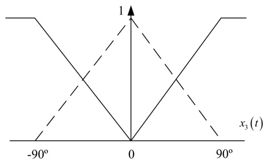
According to , the scalars , , and are found. By choosing , , and , Definition 2 is reduced as strictly input passivity focusing on the attenuation performance. Moreover, the scalars and are given. The membership is constructed as Figure 1 according to . Based on the given scalars and matrices, the following feedback gains are found by using the convex optimization algorithm to solve Theorem 2.
 and
and
Figure 1.
Membership function.
Figure 1.
Membership function.
With the obtained gains, the PDC-based fuzzy controller is established as follows:
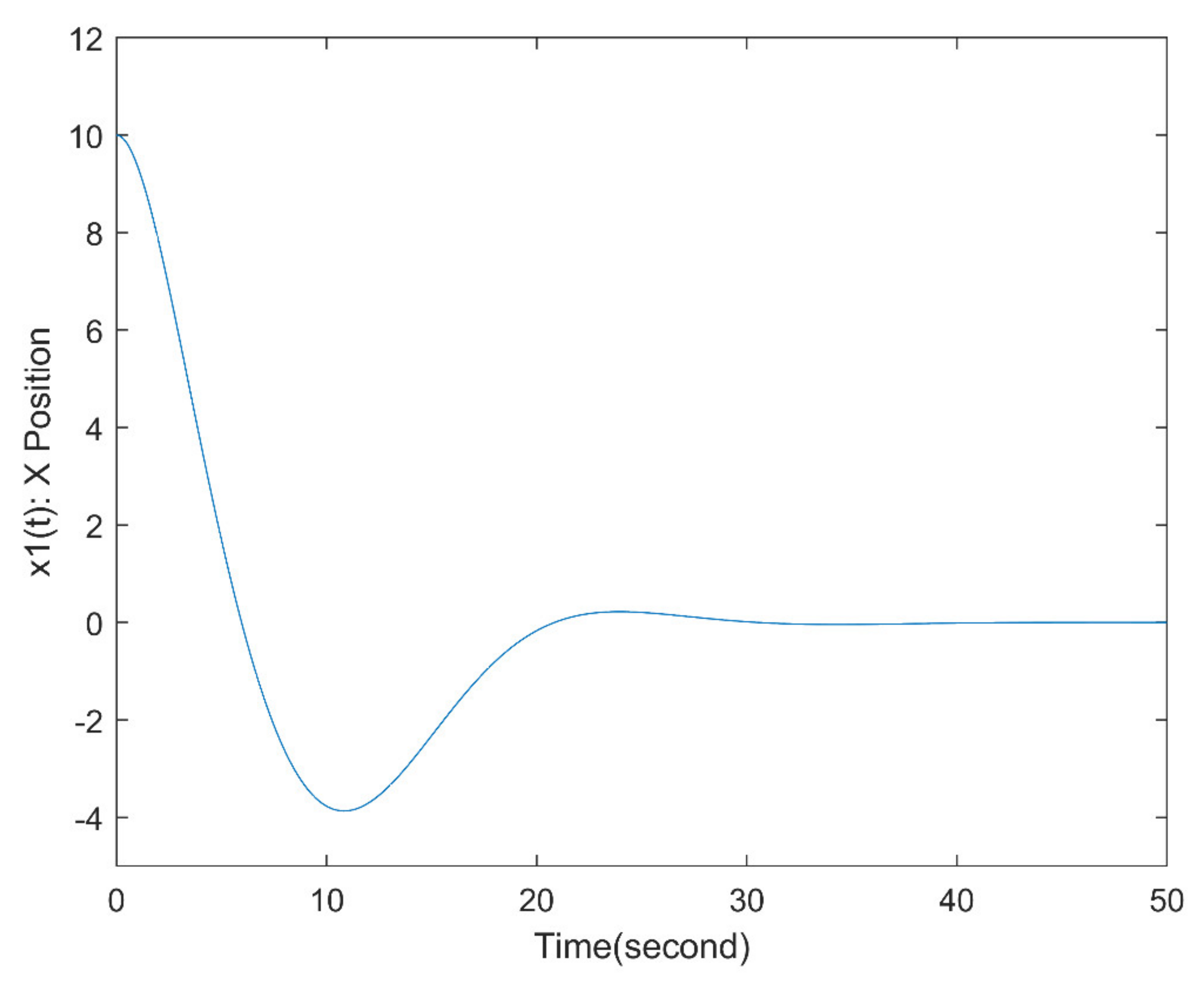
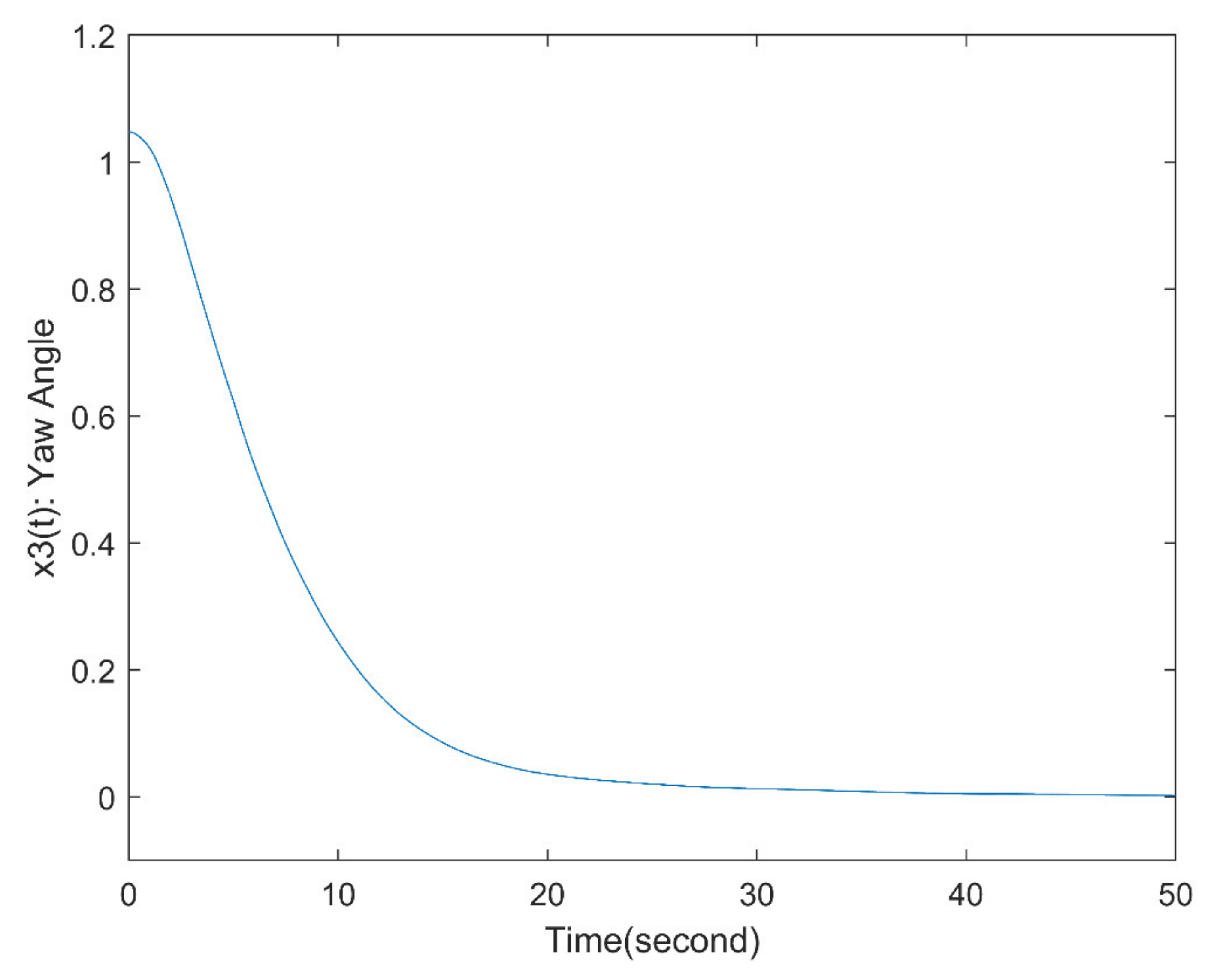
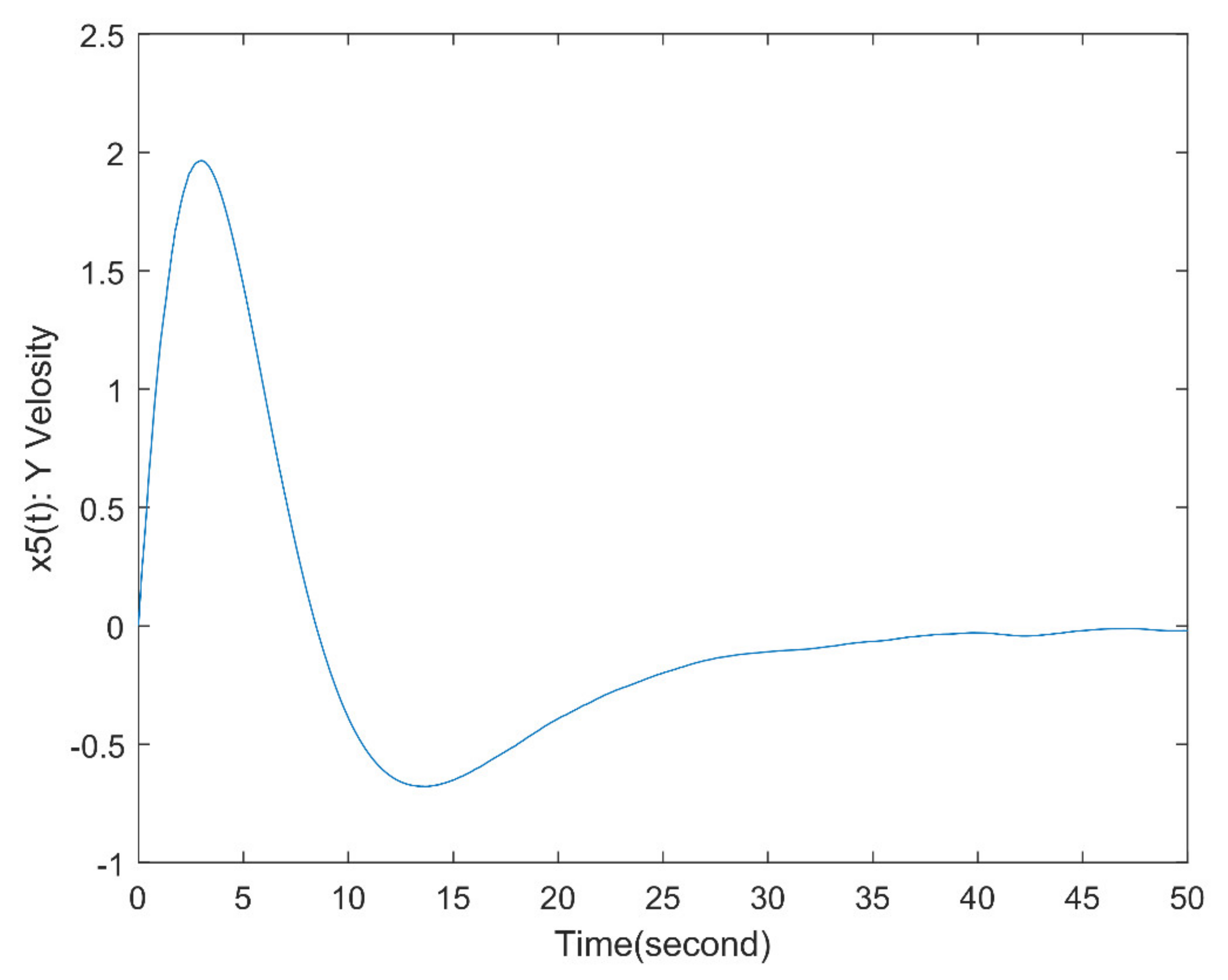
With the chosen initial condition as , the responses of the system (51)–(56) driven by (59) are showed in Figure 2, Figure 3, Figure 4, Figure 5, Figure 6 and Figure 7. According to , , , and state responses, the following equation can be applied to check the achievement of strictly input passivity.
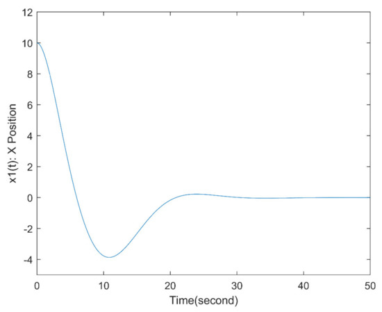
Figure 2.
Response of state .
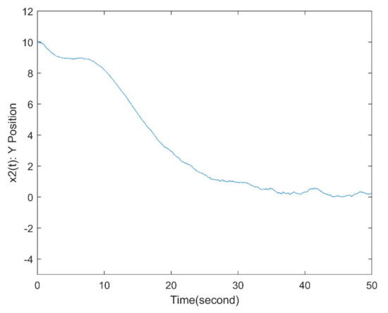
Figure 3.
Response of state .
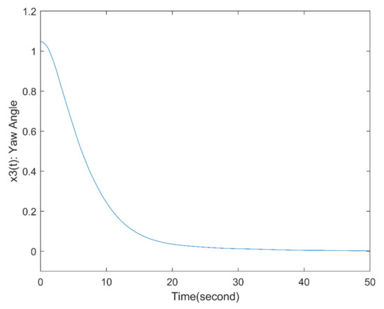
Figure 4.
Response of state .
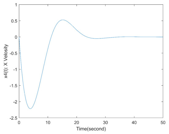
Figure 5.
Response of state .
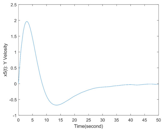
Figure 6.
Response of state .
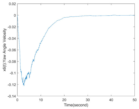
Figure 7.
Response of state .
Because the value in (60) is smaller than one, the strict input passivity of the system (51)–(56) driven by (59) is achieved by Definition 2. Referring to Figure 3, the poor transient response and vibration in are caused by external disturbance. Since the achievement in (60), the effect of an external disturbance on the system (51)–(56) is constrained by (59). Besides, the poor transient response in is made by the consideration of . From Figure 2, Figure 3, Figure 4, Figure 5, Figure 6 and Figure 7, all states of the system (51)–(56) driven by (59) are converged to zero that satisfy Definition 1. Based on the simulation results, this paper provides an effective and useful delay-dependent stability criterion to guarantee the asymptotical stability of T-S fuzzy systems with multiplicative noise in the mean square.
- Case 2
Referring to [25,26], some delay-dependent stability criteria have been proposed for delayed T-S fuzzy systems. In the literature, the parameter-independent Lyapunov-Krasovskii was applied to derive their sufficient conditions. To discuss the conservatism of searching a maximum value of delay, Theorem 1 of this paper, Corollary 1 of [25], and Theorem 1 of [26] are respectively applied to analyze the delay-dependent stability of the following T-S fuzzy system.
where , , and .
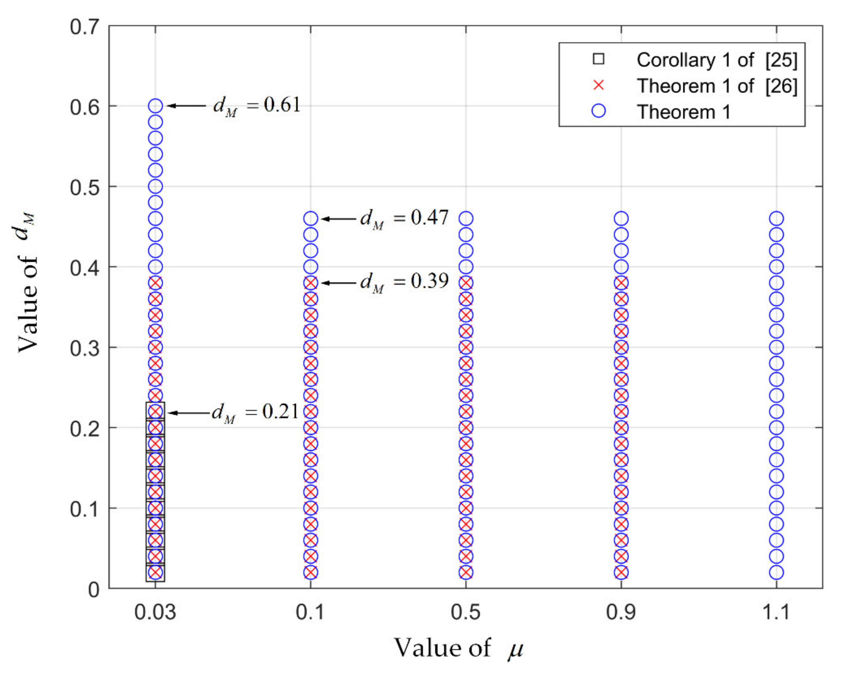
For convenience, and are set to seek the maximum value of with different values of . Therefore, four cases considered by Theorem 1 can be reduced to a single case as . By using Corollary 1 of [25], the maximum value of with is 0.21. Applying Theorem 1 of [26], the maximum value as with can be found. Based on Theorem 1 of this paper, maximum values are with and with . The comparing results are stated in Figure 8. From Figure 8, the criteria in [25,26] cannot allow the value of . Moreover, the values of found by Theorem 1 of this paper are bigger than ones found by the criteria of [25,26]. The above results mean that the number of the positive definite matrix in the Lyapunov-Krasovskii function determines relaxation. Moreover, the free-matrix inequality in Lemma 1 reduces the limitation as . Thus, it is easy to find that Theorem 1 of this paper provides a less conservative criterion than the one in [25,26] in this case.
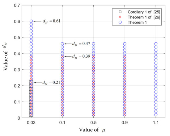
Figure 8.
Comparison result.
5. Conclusions
A delay-dependent stability criterion for nonlinear stochastic systems described by the T-S fuzzy model with multiplicative noise was investigated in this paper. To avoid conservatism during the derivative, the integral Lyapunov-Krasovskii function was proposed for deriving some sufficient conditions. To deal with the delay term during the derivative, the free-matrix inequality was employed to eliminate the limitation as . Furthermore, some lemmas were applied such that the sufficient conditions are in the strict LMI form. Moreover, some slack matrices and scalars can be introduced to increase the freedom of searching for feasible solutions. Based on the simulation results, the effectiveness and applicability of the proposed design method can be verified for guaranteeing the asymptotical stability and passivity of nonlinear systems in the mean square. Furthermore, the reduced conservatism of the proposed criterion was also discussed with the provided comparison.
Author Contributions
C.-C.K. and W.-J.C.: Conceptualization, C.-C.K. and K.-W.H.: Writing and editing, K.-W.H.: Software and data curation. All authors have read and agreed to the published version of the manuscript.
Funding
This research received no external funding.
Institutional Review Board Statement
Not applicable.
Informed Consent Statement
Not applicable.
Data Availability Statement
All relevant data displayed in publication.
Conflicts of Interest
The authors declare no conflict of interest.
References
- Wang, H.O.; Tanaka, K.; Griffin, M.F. An Approach to Fuzzy Control of Nonlinear Systems: Stability and Design Issues. IEEE Trans. Fuzzy Syst. 1996, 4, 14–23. [Google Scholar] [CrossRef]
- Chen, W.H.; Chen, B.S. Robust Stabilization Design for Nonlinear Stochastic System with Poisson Noise via Fuzzy Interpolation Method. Fuzzy Sets Syst. 2013, 217, 41–61. [Google Scholar] [CrossRef]
- Wang, F.; Chen, B.; Sun, Y.; Gao, Y.; Lin, C. Finite-Time Fuzzy Control of Stochastic Nonlinear Systems. IEEE Trans. Cybern. 2020, 50, 2617–2626. [Google Scholar] [CrossRef]
- Qi, W.; Yang, X.; Park, J.H.; Cao, J.; Cheng, J. Fuzzy SMC for Quantized Nonlinear Stochastic Switching Systems with Semi-Markovian Process and Application. IEEE Trans. Cybern. 2021, in press. [Google Scholar] [CrossRef]
- Zhang, L.; Xu, F. Controller Switching for A Class of Stochastic Fuzzy Systems. In Proceedings of the 4th International Conference on Information, Cybernetics and Computational Social Systems, Dalian, China, 24–26 July 2017. [Google Scholar]
- Chang, W.J.; Qiao, H.Y.; Ku, C.C. Sliding Mode Fuzzy Control for Nonlinear Stochastic Systems Subject to Pole Assignment and Variance Constraint. Inf. Sci. 2018, 432, 133–145. [Google Scholar] [CrossRef]
- Chang, W.J.; Hsu, F.L. Sliding Mode Fuzzy Control for Takagi-Sugeno Fuzzy Systems with Bilinear Consequent Part Subject to Multiple Constraints. Inf. Sci. 2016, 327, 258–271. [Google Scholar] [CrossRef]
- Chang, W.J.; Chen, P.H.; Ku, C.C. Variance and Passivity Constrained Sliding Mode Fuzzy Control for Continuous Stochastic Non-linear Systems. Neurocomputing 2016, 201, 29–39. [Google Scholar] [CrossRef]
- Li, M.; Shu, F.; Liu, D.; Zhong, S. Robust H∞ control of T-S Fuzzy Systems with Input Time-Varying Delays: A Delay Partitioning Method. Appl. Math. Comput. 2018, 321, 209–222. [Google Scholar] [CrossRef]
- Liu, X.D.; Zhang, Q.L. New Approaches to H∞ Controller Designs Based on Fuzzy Observers for T-S Fuzzy Systems via LMI. Automatica 2003, 39, 1571–1582. [Google Scholar]
- Wang, L.K.; Liu, X.D.; Zhang, H.G. Further Studies on H∞ Observer Design for Continuous-Time Takagi-Sugeno Fuzzy Model. Inf. Sci. 2018, 422, 396–407. [Google Scholar] [CrossRef]
- Chang, W.J.; Chang, Y.C.; Ku, C.C. Passive Fuzzy Control via Fuzzy Integral Lyapunov Function for Nonlinear Ship Drum-Boiler Systems. J. Dyn. Syst. Meas. Control ASME 2015, 137, 041008. [Google Scholar] [CrossRef] [Green Version]
- Chang, W.J.; Chen, M.W.; Ku, C.C. Passive Fuzzy Controller Design for Discrete Ship Steering Systems via Takagi-Sugeno Fuzzy Model with Multiplicative Noises. J. Mar. Sci. Technol. 2013, 21, 159–165. [Google Scholar]
- Liu, H.; Pan, Y.P.; Cao, J.; Zhou, Y.; Wang, H.X. Positivity and Stability Analysis for Fractional-Order Delayed Systems: A T-S Fuzzy Model Approach. IEEE Trans. Fuzzy Syst. 2020, in press. [Google Scholar] [CrossRef]
- Tanaka, K.; Hori, T.; Wang, H.O. A Multiple Lyapunov Function Approach to Stabilization of Fuzzy Control Systems. IEEE Trans. Fuzzy Syst. 2003, 11, 582–589. [Google Scholar] [CrossRef]
- Rhee, B.J.; Won, S.C. A New Fuzzy Lyapunov Function Approach for a Takagi-Sugeno Fuzzy Control System Design. Fuzzy Sets Syst. 2006, 157, 1211–1228. [Google Scholar] [CrossRef]
- Lee, H.J.; Park, J.B.; Chen, G.R. Robust Fuzzy Control of Nonlinear Systems with Parametric Uncertainties. IEEE Trans. Fuzzy Syst. 2001, 9, 369–379. [Google Scholar]
- Jin, X.; Chen, K.K.; Zhao, Y.; Ji, J.T.; Jing, P. Simulation of Hydraulic Transplanting Robot Control System Based on Fuzzy PID Controller. Measurement 2020, 164, 108023. [Google Scholar] [CrossRef]
- Chen, P.; Tian, Y.C. Delay-Dependent Robust Stability Criteria for Uncertain Systems with Interval Time-Varying Delay. J. Comput. Appl. Math. 2008, 214, 480–494. [Google Scholar]
- He, Y.; Wang, Q.G.; Lin, C.; Wu, M. Delay-Range-Dependent Stability for Systems with Time-Varying Delay. Automatica 2007, 43, 371–376. [Google Scholar] [CrossRef]
- Zhang, X.M.; Han, Q.L.; Seuret, A.; Gouaisbaut, F. Overview of Recent Advances in Stability of Linear Systems with Time-Varying Delays. IET Control Theory Appl. 2019, 13, 1–16. [Google Scholar] [CrossRef]
- Qi, W.; Kao, Y.G.; Gao, X.W.; Wei, Y.L. Controller Design for Time-Delay System with Stochastic Disturbance and Actuator Saturation via a New Criterion. Appl. Math. Comput. 2018, 320, 535–546. [Google Scholar] [CrossRef]
- Chen, G.L.; Xia, J.W.; Zhuang, G.M.; Zhao, J.S. Improved Delay-Dependent Stabilization for a Class of Networked Control Systems with Nonlinear Perturbations and Two Delay Components. Appl. Math. Comput. 2018, 316, 1–17. [Google Scholar] [CrossRef]
- Lien, C.H.; Yu, K.W.; Chang, H.C. Mixed Performance Analysis of Continuous Switched Systems with Time-Varying Random Delay. Asian J. Control 2020, 22, 2156–2166. [Google Scholar] [CrossRef]
- Li, C.; Wang, H.; Liao, X. Delay-Dependent Robust Stability of Uncertain Fuzzy Systems with Time-Varying Delays. IEE Proc. Control Theory Appl. 2004, 151, 417–421. [Google Scholar] [CrossRef]
- Tian, E.; Peng, C. Delay-Dependent Stability Analysis and Synthesis of Uncertain T-S Fuzzy Systems with Time-Varying Delay. Fuzzy Sets Syst. 2006, 157, 544–559. [Google Scholar] [CrossRef]
- Zhang, X.M.; Han, Q.L.; Ge, X.H.; Ding, D. An Overview of Recent Developments in Lyapunov–Krasovskii Functionals and Stability Criteria for Recurrent Neural Networks with Time-Varying Delays. Neurocomputing 2018, 313, 392–401. [Google Scholar] [CrossRef]
- Seuret, A.; Gouaisbaut, F. Wirtinger-Based Integral Inequality: Application to Time-Delay Systems. Automatica 2013, 49, 2860–2866. [Google Scholar] [CrossRef] [Green Version]
- Zeng, H.B.; He, Y.; Wu, M.; She, J.H. Free-Matrix-Based Integral Inequality for Stability Analysis of Systems with Time-Varying Delay. IEEE Trans. Autom. Control 2015, 60, 2768–2772. [Google Scholar] [CrossRef]
- Ku, C.C.; Chen, G.W. A Relaxed Observer-Based Control for LPV Stochastic Systems Subject to H∞ Performance. Int. J. Control Autom. Syst. 2020, 18, 1033–1044. [Google Scholar]
- Fossen, T.I. Guidance and Control of Ocean Vehicles; Wiley: New York, NY, USA, 1994. [Google Scholar]


Publisher’s Note: MDPI stays neutral with regard to jurisdictional claims in published maps and institutional affiliations. |
© 2021 by the authors. Licensee MDPI, Basel, Switzerland. This article is an open access article distributed under the terms and conditions of the Creative Commons Attribution (CC BY) license (https://creativecommons.org/licenses/by/4.0/).