
Accurate Determination of Electrical Potential on Ion Exchange Membranes in Reverse Electrodialysis

Abstract
:1. Introduction
2. Governing Equations and Numerical Methods
2.1. Governing Equations
2.2. Boundary Updating Scheme
2.3. Calculation of Membrane Potentials
3. Simulations and Discussion
3.1. The Effectiveness of Boundary Updating Schemne
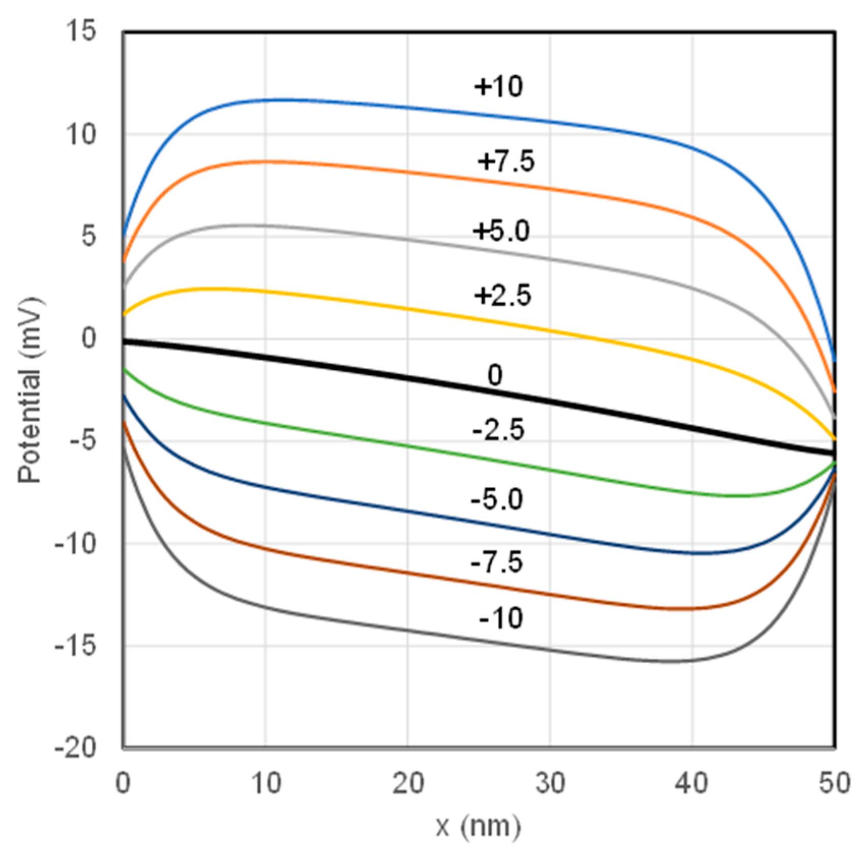
3.2. Impact of the Charge Density of IEMs
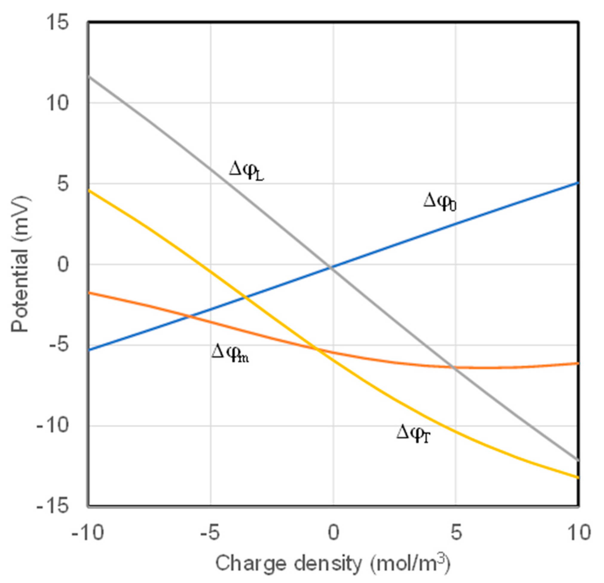
3.3. Comparison of Donnan Potentials Determinded Analytically and Numerically
3.4. The Applicability and Accuracy of TMS Model
4. Conclusions
Author Contributions
Funding
Data Availability Statement
Conflicts of Interest
References
- Mehta, G.D.; Loeb, S. Internal polarization in the porous substructure of a semipermeable membrane under pressure-retarded osmosis. J. Membr. Sci. 1978, 4, 261–265. [Google Scholar] [CrossRef]
- Lee, K.L.; Baker, R.W.; Lonsdale, H.K. Membranes for power generation by pressure-retarded osmosis. J. Membr. Sci. 1981, 8, 141–171. [Google Scholar] [CrossRef]
- Post, J.W.; Veerman, J.; Hamelers, H.V.M.; Euverink, G.J.W.; Metz, S.J.; Nymeijer, K.; Buisman, C.J.N. Salinity-gradient power: Evaluation of pressure-retarded osmosis and reverse electrodialysis. J. Membr. Sci. 2007, 288, 218–230. [Google Scholar] [CrossRef] [Green Version]
- Straub, P.; Deshmukh, A.; Elimelech, M. Pressure-retarded osmosis for power generation from salinity gradients: Is it viable? Energy Environ. Sci. 2016, 9, 31–48. [Google Scholar] [CrossRef]
- Yip, N.Y.; Vermaas, D.A.; Nijmeijer, K.; Elimelech, M. Thermodynamic, energy efficiency, and power density analysis of reverse electrodialysis power generation with natural salinity gradients. Environ. Sci. Technol. 2014, 48, 4925–4936. [Google Scholar] [CrossRef] [PubMed]
- Długołecki, P.; Nymeijer, K.; Metz, S.; Wessling, M. Current status of ion exchange membranes for power generation from salinity gradients. J. Membr. Sci. 2008, 319, 214–222. [Google Scholar] [CrossRef]
- Lacey, R.E. Energy by reverse electrodialysis. Ocean Eng. 1980, 7, 1–47. [Google Scholar] [CrossRef]
- Tedesco, M.; Hamelers, H.V.M.; Biesheuvel, P.M. Nernst-Planck transport theory for (reverse) electrodialysis: I. Effect of co-ion transport through the membranes. J. Membr. Sci. 2016, 510, 370–381. [Google Scholar] [CrossRef]
- Kim, H.; Choi, J.; Jeong, N.; Jung, Y.-G.; Kim, H.; Kim, D.; Yang, S. Correlations between properties of pore-filling ion exchange membranes and performance of a reverse electrodialysis stack for high power density. Membranes 2021, 11, 609. [Google Scholar] [CrossRef]
- Jang, H.; Kang, Y.; Han, J.-Y.; Jang, K.; Kim, C.M.; Kim, I.S. Developments and future prospects of reverse electrodialysis for salinity gradient power generation: Influence of ion exchange membranes and electrodes. Desalination 2020, 491, 114540. [Google Scholar] [CrossRef]
- Zaffora, A.; Culcasi, A.; Gurreri, L.; Cosenza, A.; Tamburini, A.; Santamaria, M.; Micale, G. Energy harvesting by waste acid/base neutralization via bipolar membrane reverse electrodialysis. Energies 2020, 13, 5510. [Google Scholar] [CrossRef]
- Teorell, T. An attempt to formulate a quantitative theory of membrane permeability. Proc. Soc. Exp. Biol. Med. 1935, 33, 282–285. [Google Scholar] [CrossRef]
- Westermann-Clark, G.B.; Christoforou, C. The exclusion-diffusion potential in charged porous membranes. J. Electroanal. Chem. Interfacial Electrochem. 1986, 198, 213–231. [Google Scholar] [CrossRef]
- Galama, A.H.; Post, J.W.; Hamelers, H.V.M.; Nikonenko, V.V.; Biesheuvel, P.M. On the origin of the membrane potential arising across densely charged ion exchange membranes: How well does the Teorell-Meyer-Sievers theory work? J. Membr. Sci. Res. 2016, 2, 128–140. [Google Scholar]
- Hodgkin, A.L.; Katz, B. The effect of sodium ions on the electrical activity of the giant axon of the squid. J. Physiol. 1949, 108, 37–77. [Google Scholar] [CrossRef]
- Feldberg, S.W. On the dilemma of the use of the electroneutrality constraint in electrochemical calculations. Electrochem. Commun. 2000, 2, 453–456. [Google Scholar] [CrossRef]
- Syganow, A.; Von Kitzing, E. (In)validity of the constant field and constant currents assumptions in theories of ion transport. Biophys. J. 1999, 76, 768–781. [Google Scholar] [CrossRef] [Green Version]
- Kato, M. Numerical analysis of the Nernst-Planck-Poisson system. J. Theor. Biol. 1995, 177, 299–304. [Google Scholar] [CrossRef]
- Blank, M. The surface compartment model: A theory of ion transport focused on ionic processes in the electrical double layers at membrane protein surfaces. Biochim. Biophys. Acta 1987, 906, 277–294. [Google Scholar] [CrossRef]
- Buck, R.P. Kinetics of bulk and interfacial ionic motion: Microscopic bases and limits for the Nernst-Planck equation applied to membrane systems. J. Membr. Sci. 1984, 17, 1–62. [Google Scholar] [CrossRef]
- Filipek, R.; Szyszkiewicz-Warzecha, K.; Bożek, B.; Danielewski, M.; Lewenstam, A. Diffusion transport in electrochemical systems: A new approach to determining of the membrane potential at steady state. Defect Diffus. Forum 2009, 283–286, 487–493. [Google Scholar] [CrossRef]
- Perrama, J.W.; Stiles, P.J. On the nature of liquid junction and membrane potentials. Phys. Chem. Chem. Phys. 2006, 8, 4200–4213. [Google Scholar] [CrossRef] [PubMed]
- Sun, Y.; Song, L. On rigorous definition of ion transport process and accurate determination of membrane potential at steady state. AIChE J. 2019, 65, e16715. [Google Scholar] [CrossRef]
- Sten-Knudsen, O. Biological Membranes: Theory of Transport, Potentials and Electric Impulses; Cambridge University Press: Cambridge, UK, 2002. [Google Scholar]


| Parameter | Symbol | Unit | Value |
|---|---|---|---|
| Membrane permittivity | F/m | 6.92 × 10⁻¹⁰ | |
| Membrane thickness | L | m | 5 × 10⁻⁸ |
| Temperature | T | K | 298.15 |
| Time step | ∆t | s | 10−9 |
| Number of spatial steps | N | 1000 | |
| Number of ions | 2 | ||
| Valence of cation | z+ | +1 | |
| Valence of anion | z− | −1 | |
| Diffusivity of cation | D+ | m2/s | 1 × 10⁻¹⁰ |
| Diffusivity of anion | D− | m2/s | 2 × 10⁻¹⁰ |
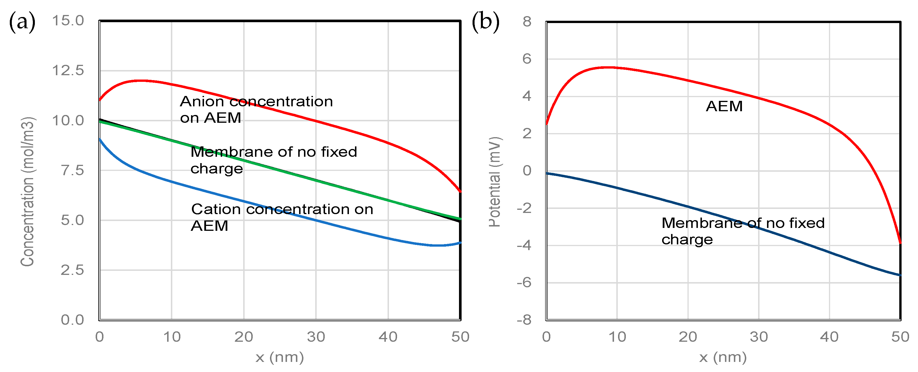
| Fixed charge | X | mol/m3 | 10 |
| Concentration on the left side | Cb0 | mol/m3 | 10 |
| Concentration on the right side | CbL | mol/m3 | 5 |
| Charge Density (mol/m3) | Δϕm (mV) | ΔϕT (mV) | Flux (mol/m2·s) |
|---|---|---|---|
| −10.00 | −1.74 | 4.61 | 1.36 × 10⁻² |
| −7.50 | −2.58 | 2.21 | 1.40 × 10⁻² |
| −5.00 | −3.57 | −0.45 | 1.41 × 10⁻² |
| −2.50 | −4.58 | −3.24 | 1.39 × 10⁻² |
| 0.00 | −5.46 | −5.94 | 1.33 × 10⁻² |
| 2.50 | −6.09 | −8.36 | 1.25 × 10⁻² |
| 5.00 | −6.38 | −10.37 | 1.15 × 10⁻² |
| 7.50 | −6.38 | −11.97 | 1.05 × 10⁻² |
| 10.00 | −6.13 | −13.20 | 9.55 × 10⁻³ |
| X (mol/m3) | Analytical | Numerical | Error (%) |
|---|---|---|---|
| −10.00 | −12.363 | −12.350 | −0.105 |
| −7.50 | −9.422 | −9.415 | −0.070 |
| −5.00 | −6.358 | −6.353 | −0.074 |
| −2.50 | −3.203 | −3.201 | −0.066 |
| 2.50 | 3.203 | 3.201 | −0.066 |
| 5.00 | 6.358 | 6.353 | −0.074 |
| 7.50 | 9.422 | 9.415 | −0.070 |
| 10.00 | 12.363 | 12.360 | −0.024 |
Publisher’s Note: MDPI stays neutral with regard to jurisdictional claims in published maps and institutional affiliations. |
© 2021 by the authors. Licensee MDPI, Basel, Switzerland. This article is an open access article distributed under the terms and conditions of the Creative Commons Attribution (CC BY) license (https://creativecommons.org/licenses/by/4.0/).
Share and Cite
Sun, Y.; Song, L. Accurate Determination of Electrical Potential on Ion Exchange Membranes in Reverse Electrodialysis. Separations 2021, 8, 170. https://doi.org/10.3390/separations8100170
Sun Y, Song L. Accurate Determination of Electrical Potential on Ion Exchange Membranes in Reverse Electrodialysis. Separations. 2021; 8(10):170. https://doi.org/10.3390/separations8100170
Chicago/Turabian StyleSun, Yuting, and Lianfa Song. 2021. "Accurate Determination of Electrical Potential on Ion Exchange Membranes in Reverse Electrodialysis" Separations 8, no. 10: 170. https://doi.org/10.3390/separations8100170