Differential Evolution in Robust Optimization Over Time Using a Survival Time Approach

Abstract

This study presents an empirical comparison of the standard differential evolution (DE) against three random sampling methods to solve robust optimization over time problems with a survival time approach to analyze its viability and performance capacity of solving problems in dynamic environments. A set of instances with four different dynamics, generated by two different configurations of two well-known benchmarks, are solved. This work also introduces a comparison criterion that allows the algorithm to discriminate among solutions with similar survival times to benefit the selection process. The results show that the standard DE holds a good performance to find ROOT solutions, improving the results reported by state-of-the-art approaches in the studied environments. Finally, it was found that the chaotic dynamic, disregarding the type of peak movement in the search space, is a source of difficulty for the proposed DE algorithm.

1. Introduction

Optimization is an inherent process in various areas of study and everyday life. The search to improve processes, services, and performances has originated in different solution techniques. However, there are problems in which uncertainty is present over time, given that the solution’s environment can change at a specific time. These types of problems are named Dynamic Optimization Problems (DOPs) [1]. This study deals with dynamic problems where the environment of the problem changes over time. Various studies have been carried out to resolve DOPs through tracking moving optima (TMO), which is characterized by the search for and implementation of the global optimal-solution every time the environment changes [2,3,4].

Evolutionary algorithms, such as Differential Evolution (DE), have shown good performance to solve tracking problems [5,6,7]. However, the search and implementation of the optimum each time the environment changes may not be feasible due to different circumstances, such as time or cost.

The approach introduced in [8] tries to solve DOPs through a procedure known as robust optimization over time (ROOT). ROOT seeks to solve DOPs by looking for a good solution for multiple environments and preserve it for as long as possible, while its quality does not decrease from a pre-established threshold. The solution found is called Robust Solution Over Time (RSOT).

In this regard, Fu et al. [9] introduced different measures to characterize environmental changes. After that, the authors developed two definitions for robustness [10]. The first one was based on “Survival Time”—when a solution is considered acceptable (an aptitude threshold must be previously defined). The second definition was based on the “Average Fitness”—the solution’s average fitness is maintained during a previously defined time window. The measurements incorporate information on the concepts of robustness and consider the values of error estimators. An algorithm performance measure was suggested to find ROOT solutions. The study was carried out using a modified version of the moving peaks benchmark (mMPB) [10].

Jin et al. [11] proposed a ROOT framework that includes three variants of the Particle Swarm Optimization algorithm (PSO). PSO with a simple restart strategy (sPSO), PSO with memory scheme (memPSO), and a variant that implements the species technique SPSO. The authors applied a radial basis function as an approximation and an autoregressive model as a predictor.

On the other hand, Wang introduced the concept of robustness in a multi-objective environment, where a framework is created to find robust Pareto fronts [12]. The author adopted the dynamic multi-objective evolutionary optimization algorithm in the experiments. At the same time, Huang et al. considered the cost derived from implementing new solutions, thus addressing the ROOT problem by a multi-objective PSO (MOPSO); The Fu metric was applied in that study [13].

Yazdani et al. introduced a new semi-ROOT algorithm that looks for a new solution when the current one is not acceptable, or if the current one is acceptable but the algorithm finds a better solution, whose implementation is preferable even with the cost of change [14].

Novoa-Hernández, Pelta, and Corona analyzed the ROOT behavior using some approximation models [15]. The authors suggested that the radial basis network model with radial basis function works better for problems with a low number of peaks. However, considering all the scenarios, the SVM model with Laplace Kernel shows notably better performance to those compared in the tests carried out.

Novoa-Hernández and Amilkar in [16] reviewed different relevant contributions to ROOT. The authors analyzed papers hosted in the SCOPUS database. Concerning new methods to solve ROOT problems, Yazdani, Nguyen, and Branke proposed a new framework using a multi-population approach where sub-populations track peaks and collect information from them [17]. Adam and Yao introduced three methods to address ROOT (Mesh, Optimal in time, and Robust). The authors mentioned that they significantly improves the results obtained for ROOT in the state-of-the-art [18]. Fox, Yang and Caraffini studied different prediction methods in ROOT, including the Linear and Quadratic Regression methods, an Autoregressive model, and Support Vector Regression [19]. Finally, Liu and Liang mapped a ROOT approach to minimize the electric bus transit center’s total cost in the first stage [20].

In different studies, DE has been used to solve ROOT problems using the Average Fitness approach, achieving competitive results [21,22]. However, to the best of the authors’ knowledge, there are no studies that determine DE’s performance in solving ROOT problems with the Survival Time approach, and this is where this work precisely focuses. This research aims to present an empirical comparison of the standard DE against three random sampling methods to solve robust optimization over time problems with a survival time approach to analyze its viability and performance capacity of solving problems in dynamic environments.

The paper is organized as follows: Section 2 includes ROOT’s definition under a survival time approach, while in Section 3 the implemented methods based on random sampling are detailed. Section 4 details the standard differential evolution and the objective function used by the algorithm in the present study. Section 5 specifies the benchmark problems to be solved. After that, Section 6 specifies the experimental settings and Section 7 shows the results obtained. Finally, Section 8 summarizes the conclusions and future work.

2. Survival Time Approach

Under this approach, a threshold is predefined to specify the quality that a solution must have to be considered good or suitable to survive. Once the threshold is defined, the search begins for a solution whose fitness can remain above the threshold in as many environments as possible. In this sense, the solution is maintained until its quality does not meet the predefined expectations, and then new robust solution over time must be sought.

In Equation (1), the function $F^s\left(\overrightarrow{x},t,V\right)$ to calculate the survival time fitness of a solution $\overrightarrow{x}$ at time t is detailed. It measures the number of environments that a solution remains in above the threshold V.

$$\begin{array}{c}\hfill F^s\left(\overrightarrow{x},t,V\right)=\left\{\begin{array}{cc}0\hfill & \mathrm{if}{f}_t\left(\overrightarrow{x}\right)<V\hfill \\ 1+max\left\{l\right|\forall i\in \{t,t+1,\dots ,t+l\}:f_i\left(\overrightarrow{x}\right)\ge V\},\hfill & \mathit{in}\mathit{other}\mathit{case}\hfill \end{array}\right.\end{array}$$

(1)

3. Random Sampling Methods

In the study presented in [18] the authors proposed three random sampling methods to solve ROOT problems, with a better performance against the state-of-the-art algorithms. The methods are described below.

In all three methods, the best solution should be searched in the current time’s solutions space, modifying the solution space when the “Robust method” is used and then using that solution next time according to the approach used (Survival Time or Average Fitness).

3.1. Mesh

This method performs random sampling in the current search space, then uses the sample with the best fitness in the current environment as a robust solution over time, using the solution found in the following times (Figure 1).

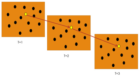
Figure 1. Mesh method. The yellow point is the robust solution found by the method and it is used in the next times.

3.2. Time-Optimal

This method performs a search similar to the “Mesh” method, with the difference that the best solution found being improved using a local search (Figure 2).

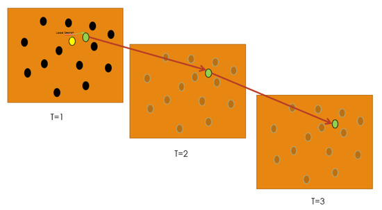
Figure 2. Time-optimal method. The green point is the robust solution found by the method, which is used in the next times.

3.3. Robust

This method performs a search similar to the “Mesh” method, differing in that a smoothing preprocessing of the solution space is performed before the search process. As seen in Figure 3, the solution obtained (green dot) can vary concerning the solution with better suitability in the raw environment (yellow dot).

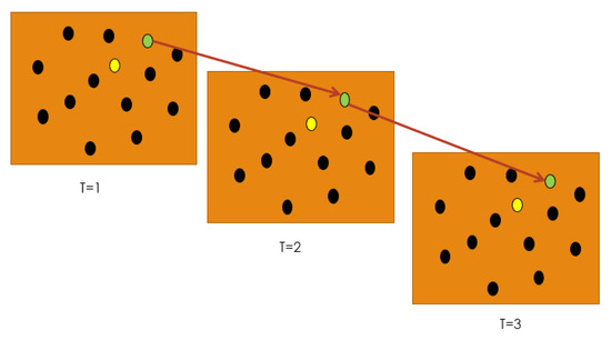
Figure 3. Robust method. The green point is the robust solution found by the method which is used in the next times.

4. Differential Evolution

In 1995, Storm and Price proposed an evolutionary algorithm to solve optimization problems in continuous spaces. DE is based on a population of solutions that, through simple recombination and mutation, evolves, thus improving individuals’ fitness [23].

Considering the fact that this work, to the best of the authors’ knowledge, is the first attempt to study DE in this type of ROOT problems (i.e., survival time), and also taking into account that the most popular DE variant (DE/rand/1/bin) has provided competitive results in ROOT problems under an average fitness approach [21,22], the algorithm used in this study is precisely the most popular variant known as DE/rand/1/bin, where ’‘rand” (random) refers to the base vector used in the mutation, ‘’bin” (binomial) refers to the crossover type used, and 1 means one vector difference computed.

The algorithm starts by randomly generating a uniformly distributed population ${\overrightarrow{x}}_i{,}_G\in i=1,\dots ,NP$, where NP is the number of individuals for each generation “G”.

After that, the algorithm enters an evolution cycle until the stop condition is reached. We applied the maximum number of evaluations allowed “$MA{X}_{Eval}$” as the stop condition.

Subsequently, to adapt individuals, the algorithm performs recombination, mutation, and the replacement of each one in the current generation. One of the most popular mutations is DE/rand/1 in Equation (2), where $r0\ne r1\ne r2\ne i$ are the indices of individuals randomly chosen from the population, 1 is the number of differences used in the mutation and $F>0$ is the scale factor.

$$\begin{array}{c}\hfill {\overrightarrow{v}}_{i,G}={\overrightarrow{x}}_{r0,G}+F({\overrightarrow{x}}_{r1,G}-{\overrightarrow{x}}_{r2,G})\end{array}$$

(2)

The vector obtained ${\overrightarrow{v}}_{i,G}$ is known as mutant vector, which is recombined with the target (parent) vector by binomial crossover, as detailed in Equation (3).

$$\begin{array}{c}\hfill u_{i,j,G}=\left\{\begin{array}{cc}{v}_{j,i,G},\hfill & if\left(ran{d}_j\le CR\right)or\left(j=j_{rand}\right)\hfill \\ x_{j,i,G},\hfill & otherwise\hfill \end{array}\right.\end{array}$$

(3)

In this study, the elements of the child vector (also called trial) $u_{i,j,G}$ are limited according to the pre-established maximum and minimum limits, also known as boundary constraints. Based on the study in [24], we use the boundary method (see Algorithm 1, line 14). In the selection process, the algorithm determines the vector that will prevail for the next generation between parent (target) and child (trial), as expressed in Equation (4).

$$\begin{array}{c}\hfill {\overrightarrow{x}}_{i,G+1}=\left\{\begin{array}{cc}{\overrightarrow{u}}_{i,G},\hfill & if\left(f\left({\overrightarrow{u}}_{i,G}\right)\le f\left({\overrightarrow{x}}_{i,G}\right)\right)\hfill \\ {\overrightarrow{x}}_{i,G},\hfill & otherwise\hfill \end{array}\right.\end{array}$$

(4)

Algorithm 1: “DE/rand/1/bin” Algorithm. NP, $MA{X}_{Eval}$, CR and F are parameters defined by the user. D is the dimension of the problem.

In Equation (1), the function to obtain an individual’s fitness through the survival time approach is shown. However, the fitness obtained is not enough to differentiate similar individuals, i.e., individuals who have survived the same amount of environments. That is why, in the implemented algorithm, we consider an additional calculation to help identify better solutions.

We propose to obtain the average of the solution’s quality in the environments that have survived. This average value helps to differentiate solutions with similar survival times. Therefore, the objective function now considers both, the number of surviving environments and the performance achieved by this solution in those environments that it has survived.

Considering the fact that the maximum height of the peaks is defined at 70 (see Table 3), the objective function for the implemented algorithm is given by the result obtained in Equation (1) multiplied by 100 plus the average fitness of the solution throughout the environments it has survived.

5. Benchmark Problems

The problems tackled in this study are based on Moving Peaks Benchmark (MPB) [25] and are configured in a similar way to that used in various specialized literature publications on ROOT, and specifically as used in [18].

Two modified MPBs can be highlighted, which are described in the following subsections. The dynamics used are presented in Table 1, where $\Delta \varphi$ is the increment from time t to time $t+1$ of the $\varphi$ parameter.

Table 1. Dynamic Functions.

1. Small Step	$\Delta \varphi =\gamma ·\parallel \varphi \parallel ·r·{\varphi }_{severity}$
2. Large Step	$\Delta \varphi =\parallel \varphi \parallel ·(\gamma *sign\left(r\right)+({\gamma }_{max}-\gamma )·r)·{\varphi }_{severity}$
3. Random	$\Delta \varphi =N(0,1)·{\varphi }_{severity}$
4. Chaotic	${\varphi }_{t+1}={\varphi }_{min}+A·({\varphi }_t-{\varphi }_{min})·(1-({\varphi }_t-{\varphi }_{min})/\parallel \varphi \parallel )$

5.1. Moving Peaks Benchmark 1 (MPB1)

In this benchmark, environments with conical peaks of height $h\left(t\right)\in [h_{min},h_{max}]$, width $w\left(t\right)\in [w_{min},w_{max}]$ and center $c\left(t\right)\in [x_{min},x_{max}]$ are generated, where the design variable x is bounded in $[x_{min},x_{max}]$. The function to generate the environment is expressed in Equation (5), where the dynamic function for height and width is given as in Table 1, while the center moves according to Equation (6). $r^i$ follows an uniform distribution of a D-dimensional sphere of radius $s^i$, and $\lambda \in [0,1]$ is a fixed parameter.

$$\begin{array}{c}\hfill f\left(\overrightarrow{x},\overrightarrow{a}\left(t\right)\right)=ma{x}_{i=1}^{i=m}\{h^i\left(t\right)-w^i\left(t\right){\parallel \overrightarrow{x}-{\overrightarrow{c}}^i\left(t\right)\parallel }_{l_2}\}\end{array}$$

(5)

$$\begin{array}{cc}\hfill {\overrightarrow{c}}^i(t+1)& ={\overrightarrow{c}}^i\left(t\right)+{\overrightarrow{v}}^i(t+1)\hfill \\ \hfill {\overrightarrow{v}}^i(t+1)& =s^i\frac{(1-\lambda )r^i(t+1)+\lambda v^i\left(t\right)}{\parallel (1-\lambda )r^i(t+1)+\lambda v^i\left(t\right)\parallel }\hfill \end{array}$$

(6)

In the present study, two problems generated by this benchmark are solved, with $\lambda =0$ it implies that the movement of the peaks is random, while with $\lambda =1$ it implies that the movement is constant in the direction ${\overrightarrow{v}}^i\left(t\right)$.

5.2. Moving Peaks Benchmark 2 (MPB2)

The set of test functions in this benchmark is described in Equation (7), where $\overrightarrow{a}\left(t\right)$ is the environment at time step t, $h^i\left(t\right),w^i\left(t\right)$, ${\overrightarrow{c}}^i\left(t\right)$ is the height, width and center of the i-th peak function at time t, respectively; $\overrightarrow{x}$ is the decision variable and m is the total number of peaks. $h^i(t+1)$ and $w^i(t+1)$ vary according to Table 1. An additional technique that uses a rotation matrix is used to rotate the centers [25].

$$\begin{array}{c}\hfill f\left(\overrightarrow{x},\overrightarrow{a}\left(t\right)\right)=\frac{1}{d}\sum _{j=1}^{d}ma{x}_{i=1}^{i=m}\{h^i\left(t\right)-w^i\left(t\right)\parallel \overrightarrow{x}-{\overrightarrow{c}}^i\left(t\right)\parallel \}\end{array}$$

(7)

6. Experimental Settings

Based on the information in Section 5, different environments are generated as test problems and they are summarized in Table 2.

Table 2. Summary of problems.

Benchmark	Abbreviation	Configuration	Dynamic ($\mathit{\delta }$)
MPB1	$B1D\delta -1$	$\lambda =0$	{1,2,3,4}
MPB1	$B1D\delta -2$	$\lambda =1$	{1,2,3,4}
MPB2	$B2D\delta -a$	uniform start of peak distribution	{1,2,3,4}
MPB2	$B2D\delta -b$	random start of peak distribution	{1,2,3,4}

The parameter settings of the problems are detailed in Table 3.

Table 3. Parameters settings.

Parameter	MPB1	MBP2
Number of peaks m	5	25
Number of dimensions d	2	2
Search range $[x_{min},x_{max}]$	$[0,50]$	$[-25,25]$
Height range $[h_{min},h_{max}]$	$[30,70]$	$[30,70]$
Width range $[w_{min},w_{max}]$	$[1,12]$	$[1,13]$
Angle range $[{\theta }_{min},{\theta }_{max}]$	-	$[-\pi ,\pi ]$
$heigh{t}_{severity}$	$U(1,10)$	5.0
$widt{h}_{severity}$	$U(0.1,1)$	0.5
$angl{e}_{severity}$	-	1.0
Initial h	50	$U(h_{min},h_{max})$
Initial w	6	$U(w_{min},w_{max})$
Initial Angle	-	0
$\lambda$	$\{0,1\}$	-
Number of dimensions for rotation $l_r$	-	2
Computational budget at each step $\Delta e$	2500	2500

The height and width of the peaks were randomly initialized in the predefined ranges. The centers were randomly initialized within the solution space.

A survival threshold $V=$ 50 is selected, representing the most difficult cases that have been resolved in the literature under the survival approach. The higher the survival threshold, the more difficult it is to find solutions that satisfy multiple scenarios.

The DE parameters were fine-tuned using the iRace tool [26] and they are summarized in Table 4, where NP is the population size, CR is the crossover parameter, and F is the scale factor.

Table 4. Parameter settings of DE.

NP	CR	F
54	0.53	0.73

For each problem, a solution is sought at each time $t\in (2,\dots ,100)$.

In order to evaluate an RSOT in a specific time, approximate and predictive methods have been used in the literature so that the performance of an algorithm depends on their accuracy. However, in this study, we want to know the DE behavior when solving the ROOT environments considering they had ideal predictors to evaluate the solutions. In this regard, the process to study the algorithm’s ability to find RSOT using DE at each instant of time is as follows:

• A solution is sought according to the algorithm described in Section 4, and the measured solution value by Equation (1) is recorded.
• Subsequently, to obtain the algorithm’s performance in the following environment, the search process is performed again using the real-environments; the best solution found is newly measured by Equation (1) and is also recorded.
• The described procedure is carried out at each instant of time that is being recorded. Therefore, in the present study, it is not necessary to detect environmental changes to know at what point in time a solution is no longer considered good. Each time a solution is sought, the algorithm initializes its population randomly, avoiding diversity problems.

7. Results and Discussion

The results for the problems generated with dynamics 1–4 are detailed in Table 7 and graphically shown in Figures 6–9, for each one of the four dynamics. In all four figures, those labeled with (a) and (b) present the results obtained in the MPB1 problems, while those labeled with (c) and (d) refer to the MPB2 problems. In all cases, the average survival values obtained by Mesh, time-optimal and robust approaches are compared against DE.

Non-parametric statistical tests [27] were applied to the corresponding numerical results presented in Table 7. The $95\%$-confidence Kruskal–Wallis and $95\%$-confidence Friedman tests were applied and their obtained p-values are reported in Table 5.

Table 5. Results of the $95\%$-confidence Kruskal–Wallis (KW) and Friedman (F) tests. The symbol (*) after letter ‘’D” in the Problem column refers to the type of dynamic used according to columns Dynamic. A p-value less than 0.05 means that there are significant differences among the compared algorithms in such problems.

Problem Instance	p-Value
	Dynamic 1		Dynamic 2		Dynamic 3		Dynamic 4
	KW	F	KW	F	KW	F	KW	F
B1D*-1	<0.0001	<0.0001	<0.0001	<0.0001	<0.0001	<0.0001	<0.0001	<0.0001
B1D*-2	<0.0001	<0.0001	<0.0001	<0.0001	<0.0001	<0.0001	0.0082	<0.0001
B2D*-a	<0.0001	<0.0001	<0.0001	<0.0001	<0.0001	<0.0001	<0.0001	<0.0001
B2D*-b	<0.0001	<0.0001	<0.0001	<0.0001	<0.0001	<0.0001	<0.0001	<0.0001

To further determine differences among the compared algorithms, the $95\%$-confidence Wilcoxon test was applied to pair-wise comparisons for each problem instance. The obtained p-values are reported in Table 6, where the significant improvement with a significance level $\alpha =0.5$ is shown in boldface. We can observe that the Wilcoxon test confirmed significant differences obtained in Kruskal–Wallis and Friedman Tests, most of them comparing DE/rand/1/bin versus random sampling methods, with the exception of four corresponding to problems generated with dynamic 4 (B1D4-1 and B1D4-2 both, in the comparison of DE/rand/1/bin versus Mesh and DE/rand/1/bin versus Time-optimal).

Table 6. Results of the $95\%$-confidence Wilcoxon signed-rank test. A p-value less than 0.05 means that exists significant differences.

Problem	Algorithm	p-Value
		Dynamic 1	Dynamic 2	Dynamic 3	Dynamic 4
B1D*-1	DE/rand/1/bin versus Mesh	<0.0001	<0.0001	<0.0001	0.2545
	DE/rand/1/bin versus Time-optimal	<0.0001	<0.0001	<0.0001	0.2881
	DE/rand/1/bin versus Robust	<0.0001	<0.0001	<0.0001	<0.0001
	Mesh versus Time-optimal	0.1167	0.0019	0.0483	0.8758
	Mesh versus Robust	<0.0001	0.0006	0.1019	<0.0001
	Time-optimal versus Robust	<0.0001	<0.0001	0.0007	<0.0001
B1D*-2	DE/rand/1/bin versus Mesh	<0.0001	<0.0001	<0.0001	0.7724
	DE/rand/1/bin versus Time-optimal	<0.0001	<0.0001	<0.0001	0.7531
	DE/rand/1/bin versus Robust	<0.0001	<0.0001	<0.0001	0.0037
	Mesh versus Time-optimal	0.9602	0.9358	0.8852	0.9984
	Mesh versus Robust	0.0987	0.9078	0.0087	0.0067
	Time-optimal versus Robust	0.104	0.8558	0.0126	0.0069
B2D*-a	DE/rand/1/bin versus Mesh	<0.0001	<0.0001	<0.0001	<0.0001
	DE/rand/1/bin versus Time-optimal	<0.0001	<0.0001	<0.0001	<0.0001
	DE/rand/1/bin versus Robust	<0.0001	<0.0001	<0.0001	<0.0001
	Mesh versus Time-optimal	0.8796	0.6044	0.8479	0.9221
	Mesh versus Robust	0.5502	0.9639	<0.0001	0.761
	Time-optimal versus Robust	0.4222	0.5658	<0.0001	0.7259
B2D*-b	DE/rand/1/bin versus Mesh	<0.0001	<0.0001	<0.0001	<0.0001
	DE/rand/1/bin versus Time-optimal	<0.0001	<0.0001	<0.0001	<0.0001
	DE/rand/1/bin versus Robust	<0.0001	<0.0001	<0.0001	<0.0001
	Mesh versus Time-optimal	0.7937	0.9805	0.6242	0.9028
	Mesh versus Robust	0.7231	0.6922	0.0001	0.3679
	Time-optimal versus Robust	0.8786	0.6761	0.0014	0.3369

Table 7 summarizes the mean and standard deviation statistical results obtained by the compared algorithms. It can be seen that DE/rand/1/bin obtains the highest average values in all the problems that were solved. Nevertheless, the higher standard deviation values obtained by DE/rand/1/bin in problems B1D4-1 and B1D4-2 confirm those expressed by the non-parametric tests—the differences are not significant with respect to the random sampling methods. Figure 4 and Figure 5 have the box-plots for B1D4-1 and B1D4-2, where all the compared algorithms reach survival times between 1 and 3, with the exception of the Robust approach in B1D4-1, but such a difference was not significant.

Table 7. Statistical Results obtained by each Algorithm in each one of the problem instances. Best statistical results are marked with boldface.

Problem	Algorithm	Dynamic 1		Dynamic 2		Dynamic 3		Dynamic 4
		Mean	S.D.	Mean	S.D.	Mean	S.D.	Mean	S.D.
B1D*-1	DE/rand/1/bin	10.1438	1.5056	6.1306	0.6816	10.6581	1.4973	1.5678	1.7595
	Mesh	4.9337	0.7772	2.9772	0.3448	5.6844	0.8894	0.9429	0.8177
	Time-optimal	5.0527	0.7756	3.0365	0.3503	5.7979	0.8857	0.9569	0.8728
	Robust	4.4819	0.7853	2.8947	0.3577	5.5371	0.9837	0.3176	0.2515
B1D*-2	DE/rand/1/bin	13.5633	3.866	8.623	2.1388	13.8394	3.6942	1.8219	1.9531
	Mesh	10.329	4.0575	5.6162	1.8619	10.5887	3.9488	1.7269	1.8693
	Time-optimal	10.3309	4.0328	5.6104	1.8461	10.5731	3.923	1.7235	1.8584
	Robust	10.1437	3.9241	5.6533	1.8166	10.2246	3.7413	1.2843	1.4648
B2D*-a	DE/rand/1/bin	19.1757	0.1236	19.8474	0.0399	19.381	0.0748	18.0117	0.3944
	Mesh	6.596	0.7258	6.5154	0.26	6.3956	0.3199	2.7558	0.229
	Time-optimal	6.5914	0.7413	6.5321	0.2713	6.4116	0.3177	2.7593	0.2315
	Robust	6.6709	0.7904	6.5109	0.2611	6.1947	0.2593	2.7411	0.2276
B2D*-b	DE/rand/1/bin	16.9954	0.4005	18.1336	0.1144	17.7187	0.1345	13.1993	0.8169
	Mesh	5.5729	0.8528	5.2304	0.3239	4.8788	0.2544	2.2192	0.3461
	Time-optimal	5.5825	0.836	5.233	0.3227	4.868	0.2463	2.2238	0.3472
	Robust	5.6479	0.981	5.215	0.3266	4.7578	0.2359	2.1818	0.334

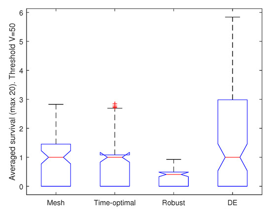
Figure 4. Boxplot of the results obtained in B1D4-1.

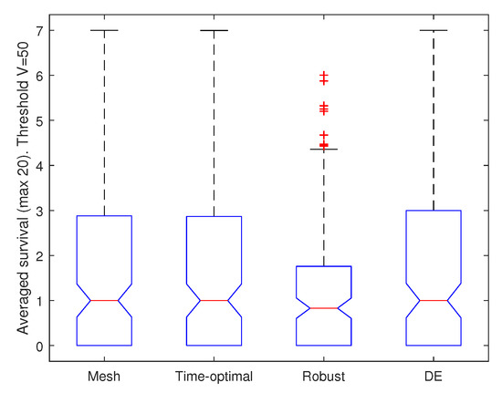
Figure 5. Boxplot of the results obtained in B1D4-2.

With respect to the graphical results, when MPB1 (items (a) and (b)) is compared against MPB2 (items (c) and (d)) in Figure 6, Figure 7, Figure 8 and Figure 9, it is clear that MPB1 is more difficult to solve by all four approaches. However, in all cases (MPB1 and MPB2 in the four dynamics) DE is able to provide better results against the three other algorithms. Such a performance is more evident in all MPB2 instances.

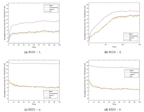
Figure 6. Results obtained using dynamic 1.

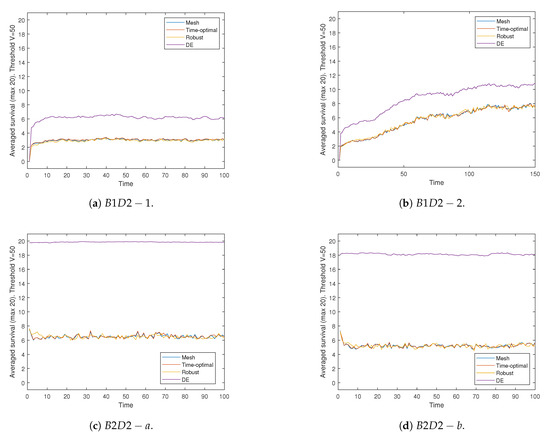
Figure 7. Results obtained using dynamic 2.

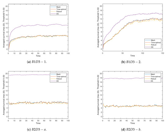
Figure 8. Results obtained using dynamic 3.

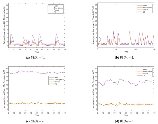
Figure 9. Results obtained using dynamic 4.

Regarding MPB1 (items (a) and (b)), it is important to note that it is more difficult to find higher survival times when the peak movement is random (items (a), where $\lambda$ = 0).

Another interesting behavior found is that all four compared methods are affected mainly by the random and chaotic dynamics in those MPB1 instances, the latter one being the most complex (chaotic dynamic). However, even in such a case DE was able to match and in some cases improve the survival values of the compared approaches. This source of difficulty now found motivates part of our future research.

8. Conclusions

A performance analysis of the differential evolution algorithm, with one of its original variants, called DE/rand/1/bin, when solving robust optimization over time problems with a survival time approach, was presented in this paper. Three state-of-the-art random sampling methods to solve ROOT problems were used for comparison purposes. Sixteen generated problems by two benchmarks with two configurations and four different dynamics were solved. The solutions generated by the DE were obtained using the real environments without prediction mechanisms with the aim to analyze its behavior in ideal conditions. The findings supported by the obtained results indicate that DE is a suitable algorithm to deal with this type of dynamic search space when a survival time approach is considered. Moreover, the additional criterion that was added to the DE objective function allowed the algorithm to better discriminate between similar solutions in terms of survival time. Furthermore, it was found that the combination of a chaotic dynamic with both, random and constant peak movements, is a source of difficulty that requires further analysis.

This last finding is the starting point of our future research, where more recent DE variants, such as DE/current-to-p-best, will be tested in those complex ROOT instances. Moreover, the effect of predictors in DE-based approaches will be studied.

References

- Nguyen, T.T.; Yang, S.; Branke, J. Evolutionary dynamic optimization: A survey of the state of the art. Swarm Evolut. Comput. 2012, 6, 1–24. [Google Scholar] [CrossRef]
- Dang, D.C.; Jansen, T.; Lehre, P.K. Populations Can Be Essential in Tracking Dynamic Optima. Algorithmica 2017, 78, 660–680. [Google Scholar] [CrossRef] [PubMed]
- Yang, S.; Li, C. A clustering particle swarm optimizer for locating and tracking multiple optima in dynamic environments. IEEE Trans. Evolut. Comput. 2010, 14, 959–974. [Google Scholar] [CrossRef]
- Yang, S.; Yao, X. Evolutionary Computation for Dynamic Optimization Problems; Springer: Berlin/Heidelberg, Germany, 2013. [Google Scholar] [CrossRef]
- Das, S.; Mullick, S.S.; Suganthan, P. Recent advances in differential evolution—An updated survey. Swarm Evolut. Comput. 2016, 27, 1–30. [Google Scholar] [CrossRef]
- Lin, L.; Zhu, M. Efficient Tracking of Moving Target Based on an Improved Fast Differential Evolution Algorithm. IEEE Access 2018, 6, 6820–6828. [Google Scholar] [CrossRef]
- Zhu, Z.; Chen, L.; Yuan, C.; Xia, C. Global replacement-based differential evolution with neighbor-based memory for dynamic optimization. Appl. Intell. 2018, 48, 3280–3294. [Google Scholar] [CrossRef]
- Yu, X.; Jin, Y.; Tang, K.; Yao, X. Robust optimization over time; A new perspective on dynamic optimization problems. In Proceedings of the IEEE Congress on Evolutionary Computation, Barcelona, Spain, 18–23 July 2010; pp. 1–6. [Google Scholar] [CrossRef]
- Fu, H.; Sendhoff, B.; Tang, K.; Yao, X. Characterizing environmental changes in Robust Optimization Over Time. In Proceedings of the IEEE Congress on Evolutionary Computation, Brisbane, QLD, Australia, 10–15 June 2012; pp. 1–8. [Google Scholar] [CrossRef]
- Fu, H.; Sendhoff, B.; Tang, K.; Yao, X. Finding Robust Solutions to Dynamic Optimization Problems. In Applications of Evolutionary Computation; Esparcia-Alcázar, A.I., Ed.; Springer: Berlin/Heidelberg, Germany, 2013; pp. 616–625. [Google Scholar]
- Jin, Y.; Tang, K.; Yu, X.; Sendhoff, B.; Yao, X. A framework for finding robust optimal solutions over time. Memetic Comput. 2013, 5, 3–18. [Google Scholar] [CrossRef]
- Wang, H.L.G.C. The Evolutionary Algorithm to Find Robust Pareto-Optimal Solutions over Time. Math. Probl. Eng. 2014, 2014, 814210. [Google Scholar]
- Huang, Y.; Ding, Y.; Hao, K.; Jin, Y. A multi-objective approach to robust optimization over time considering switching cost. Inf. Sci. 2017, 394–395, 183–197. [Google Scholar] [CrossRef]
- Yazdani, D.; Branke, J.; Omidvar, M.N.; Nguyen, T.T.; Yao, X. Changing or Keeping Solutions in Dynamic Optimization Problems with Switching Costs. In Proceedings of the Genetic and Evolutionary Computation Conference, Kyoto, Japan, 15–19 July 2018; pp. 1095–1102. [Google Scholar] [CrossRef]
- Novoa-Hernández, P.; Pelta, D.A.; Corona, C.C. Approximation Models in Robust Optimization Over Time—An Experimental Study. In Proceedings of the 2018 IEEE Congress on Evolutionary Computation (CEC), Rio de Janeiro, Brazil, 8–13 July 2018; pp. 1–6. [Google Scholar] [CrossRef]
- Novoa-Hernández, P.; Puris, A. Robust optimization over time: A review of most relevant contributions [Optimización robusta en el tiempo: Una revisión de las contribuciones más relevantes]. Rev. Iber. Sist. Tecnol. Inf. 2019, 2019, 156–164. [Google Scholar]
- Yazdani, D.; Nguyen, T.T.; Branke, J. Robust Optimization Over Time by Learning Problem Space Characteristics. IEEE Trans. Evolut. Comput. 2019, 23, 143–155. [Google Scholar] [CrossRef]
- Adam, L.; Yao, X. A Simple Yet Effective Approach to Robust Optimization Over Time. In Proceedings of the 2019 IEEE Symposium Series on Computational Intelligence (SSCI), Xiamen, China, 6–9 December 2019; pp. 680–688. [Google Scholar]
- Fox, M.; Yang, S.; Caraffini, F. An Experimental Study of Prediction Methods in Robust optimization Over Time. In Proceedings of the 2020 IEEE Congress on Evolutionary Computation (CEC), Glasgow, UK, 19–24 July 2020; pp. 1–7. [Google Scholar]
- Liu, Y.; Liang, H. A ROOT Approach for Stochastic Energy Management in Electric Bus Transit Center with PV and ESS. In Proceedings of the 2019 IEEE Global Communications Conference (GLOBECOM), Waikoloa, HI, USA, 9–13 December 2019; pp. 1–6. [Google Scholar]
- Guzmán-Gaspar, J.; Mezura-Montes, E. Differential Evolution Variants in Robust Optimization Over Time. In Proceedings of the 2019 International Conference on Electronics, Communications and Computers (CONIELECOMP), Cholula, Mexico, 27 February–1 March 2019; pp. 164–169. [Google Scholar]
- Guzmán-Gaspar, J.; Mezura-Montes, E. Robust Optimization Over Time with Differential Evolution using an Average Time Approach. In Proceedings of the 2019 IEEE Congress on Evolutionary Computation (CEC), Wellington, New Zealand, 10–13 June 2019; pp. 1548–1555. [Google Scholar]
- Price, K.; Storn, R.M.; Lampinen, J.A. Differential Evolution a Practical Approach to Global Optimization, 1st ed.; Springer: Berlin/Heidelberg, Germany, 2005. [Google Scholar]
- Juárez-Castillo, E.; Acosta-Mesa, H.G.; Mezura-Montes, E. Adaptive boundary constraint-handling scheme for constrained optimization. Soft Comput. 2019, 23, 8247–8280. [Google Scholar] [CrossRef]
- Li, C.; Yang, S.; Nguyen, T.T.; Yu, E.L.; Yao, X.; Jin, Y.; Beyer, H.G.; Suganthan, P.N. Benchmark Generator for CEC 2009 Competition on Dynamic Optimization. Available online: https://bura.brunel.ac.uk/bitstream/2438/5897/2/Fulltext.pdf (accessed on 24 October 2020).
- López-Ibáñez, M.; Dubois-Lacoste, J.; Pérez Cáceres, L.; Birattari, M.; Stützle, T. The irace package: Iterated racing for automatic algorithm configuration. Oper. Res. Perspect. 2016, 3, 43–58. [Google Scholar] [CrossRef]
- García, S.; Molina, D.; Lozano, M.; Herrera, F. A Study on the Use of Non-Parametric Tests for Analyzing the Evolutionary Algorithms’ Behaviour: A Case Study on the CEC’2005 Special Session on Real Parameter Optimization. J. Heuristics 2009, 15, 617–644. [Google Scholar] [CrossRef]
Publisher’s Note: MDPI stays neutral with regard to jurisdictional claims in published maps and institutional affiliations. |
© 2020 by the authors. Licensee MDPI, Basel, Switzerland. This article is an open access article distributed under the terms and conditions of the Creative Commons Attribution (CC BY) license (http://creativecommons.org/licenses/by/4.0/).