The Generalized Odd Linear Exponential Family of Distributions with Applications to Reliability Theory

Abstract

A new family of continuous distributions called the generalized odd linear exponential family is proposed. The probability density and cumulative distribution function are expressed as infinite linear mixtures of exponentiated-F distribution. Important statistical properties such as quantile function, moment generating function, distribution of order statistics, moments, mean deviations, asymptotes and the stress–strength model of the proposed family are investigated. The maximum likelihood estimation of the parameters is presented. Simulation is carried out for two of the mentioned sub-models to check the asymptotic behavior of the maximum likelihood estimates. Two real-life data sets are used to establish the credibility of the proposed model. This is achieved by conducting data fitting of two of its sub-models and then comparing the results with suitable competitive lifetime models to generate conclusive evidence.

1. Introduction

Analysis of lifetime data is an important subject in many fields, including reliability, social sciences, biomedical, engineering and other fields. In practice, it has been observed that many phenomena do not follow any of the classical distributions; for this reason, many efforts have been made in the last few decades to introduce new generators or families of distributions that extend these classical distributions to provide considerable flexibility in modeling data in diverse spectrums. Many authors have suggested new generators or families in the literature, for example, and not exclusively: Marshall and Olkin (1997) [1] introduced the Marshall–Olkin family, Gupta et al. (1998) [2] introduced the exponentiated-G family, Eugene et al. (2002) [3] proposed the beta-G family, Cordeiro and Castro (2011) [4] suggested the Kumaraswamy-G family, Alexander et al. (2012) [5] presented the McDonald-G family, Alzaatreh et al. (2013) [6] proposed the transformed-transformer (T-X) family, Bourguignon et al. (2014) [7] presented the Weibull-G family, Tahir et al. (2015) [8] studied the odd generalized exponential-G family, Cordeiro et al. (2016) [9] discussed the Zografos Balakrishnan odd log-logistic family, Gomes-Silva et al. (2017) [10] presented the odd Lindley-G family, Alizadeh et al. (2017) [11] provided the Gompertz-G family and Jamal et al. (2017) [12] defined the odd Burr-III family, among others. For a clearer understanding of the odds ratio to define new G-classes, we motivate the readers to Khan et al. (2021) [13], in which the authors adopted a unique odd function to propose an alternate generalized odd generalized exponential-G family.

The linear exponential or (linear failure rate) distribution is the distribution of the minimum of two independent random variables Z₁ and Z₂ having exponential (a) and Rayleigh (b) (Sen and Bhattacharyya, 1995 [14]). Therefore, the variables have exponential and Rayleigh distributions as special cases, which are well-known distributions for modeling lifetime data in reliability and medical studies. The linear exponential distribution is used to model phenomena with linearly increasing failure rates, but it does not provide a reasonable fit for modeling phenomena with decreasing, non-linear increasing, or non-monotonic failure rates, which include the bathtub and upside-down bathtub, among others. These phenomena are common in reliability and biological studies. This motivated us to introduce generalizations of linear, exponential distribution so that their goodness of fit measures may improve the tail properties. Our motivations and the main goals of this paper are to propose a random variable that follows the linear exponential distribution as a new generator to introduce new models which can yield all types of the hazard rate functions with improved goodness of fit properties for real-life data.

2. The Generalized Odd Linear Exponential (GOLE-F) Family

Suppose the random variable $Z$ has a linear exponential distribution with parameters $a,b\ge 0$ where $a+b>0$, then its cumulative distribution function (CDF) and probability density function (PDF) are, respectively,

$$R\left(z\right)=1-e^{-\left(az+\frac{b}{2}{z}^2\right)}, z\ge 0$$

(1)

$$r\left(z\right)=\left(a+bz\right)e^{-\left(az+\frac{b}{2}{z}^2\right)}. z>0.$$

(2)

Adopting the T-X framework defined by the authors in [6], for any power parameter $c>0,$ we define the CDF of a new wider family called the generalized odd linear exponential (“GOLE-F” for short) family by

$$G\left(x;a,b,c,\mathit{\varphi }\right)={{\displaystyle \int }}_0^{\frac{F{\left(x;\mathit{\varphi }\right)}^c}{1-F{\left(x;\mathit{\varphi }\right)}^c}}\left(a+bz\right)e^{-\left(az+\frac{b}{2}{z}^2\right)}dz=1-\exp \left[-\left(\frac{aF{\left(x;\mathit{\varphi }\right)}^c}{1-F{\left(x;\mathit{\varphi }\right)}^c}+\frac{b}{2}{\left(\frac{F{\left(x;\mathit{\varphi }\right)}^c}{1-F{\left(x;\mathit{\varphi }\right)}^c}\right)}^2\right)\right],$$

(3)

where $W\left[F\left(x\right)\right]=\frac{F{\left(x;\mathit{\varphi }\right)}^c}{1-F{\left(x;\mathit{\varphi }\right)}^c}$ is the link function with $F\left(x;\mathit{\varphi }\right)$ as the baseline CDF of an absolutely continuous distribution with parameter vector $\mathit{\varphi }$ and pdf $f\left(x;\mathit{\varphi }\right)$.

The PDF of GOLE-F corresponding to the CDF in Equation (3) is provided by

$$g\left(x;a,b,c,\mathit{\varphi }\right)=\left[\frac{cf\left(x;\mathit{\varphi }\right)F{\left(x;\mathit{\varphi }\right)}^{c-1}\left(a+\left(b-a\right)F{\left(x;\mathit{\varphi }\right)}^c\right)}{{\left(1-F{\left(x;\mathit{\varphi }\right)}^c\right)}^3}\right]\times \exp \left[-\left(\frac{aF{\left(x;\mathit{\varphi }\right)}^c}{1-F{\left(x;\mathit{\varphi }\right)}^c}+\frac{b}{2}{\left(\frac{F{\left(x;\mathit{\varphi }\right)}^c}{1-F{\left(x;\mathit{\varphi }\right)}^c}\right)}^2\right)\right].$$

(4)

Henceforth, for any parent model, we will simply write $F\left(x\right)=F\left(x;\mathit{\varphi }\right)$ as the distribution function and $f\left(x\right)=f\left(x;\mathit{\varphi }\right)$ as the density function. Further, any random variable $X$ with density function (4) is denoted by $X~GOLE-F \left(a,b,c,\mathit{\varphi }\right)$.

The hazard rate function (HRF) and reversed hazard rate function (RHRF) of the random variable $X$ are, respectively,

$$h\left(x;a,b,c,\mathit{\varphi }\right)=\frac{cf\left(x\right)F{\left(x\right)}^{c-1}\left(a+\left(b-a\right)F{\left(x\right)}^c\right)}{{\left(1-F{\left(x\right)}^c\right)}^3},$$

(5)

and

$$\tau \left(x;a,b,c,\mathit{\varphi }\right)=\frac{\left\{cf\left(x\right)F{\left(x\right)}^{c-1}\left(a+\left(b-a\right)F{\left(x\right)}^c\right)\right\}{e}^{-\left(\frac{aF{\left(x\right)}^c}{1-F{\left(x\right)}^c}+\frac{b}{2}{\left(\frac{F{\left(x\right)}^c}{1-F{\left(x\right)}^c}\right)}^2\right)}}{{\left(1-F{\left(x\right)}^c\right)}^3\left\{1-e^{-\left(\frac{aF{\left(x\right)}^c}{1-F{\left(x\right)}^c}+\frac{b}{2}{\left(\frac{F{\left(x\right)}^c}{1-F{\left(x\right)}^c}\right)}^2\right)}\right\}}.$$

(6)

The quantile function of the random variable $X$ can be obtained by inverting Equation (3), and hence the GOLE-F distribution can be simulated easily from the following Equation.

$$X=Q\left(U\right)=F^{-1}\left({\left[\frac{-a+\sqrt{a^2-2b\log \left(1-U\right)}}{b-a+\sqrt{a^2-2b\log \left(1-U\right)}}\right]}^{1/c}\right),$$

(7)

where $U$ has a uniform distribution over the interval (0,1), in particular, if $u=1/2$ we obtain the median of the random variable $X$ as follows:

$$M=Q\left(\frac{1}{2}\right)=F^{-1}\left({\left[\frac{-a+\sqrt{a^2-2b\log \left(1-1/2\right)}}{b-a+\sqrt{a^2-2b\log \left(1-1/2\right)}}\right]}^{1/c}\right).$$

(8)

3. Special Model of the GOLE-F Family

In this section, we provide two extended distributions as special models of the GOLE-F family and display their plots of density and hazard rate functions.

3.1. The Generalized Odd Linear Exponential-Weibull (GOLE-W) Distribution

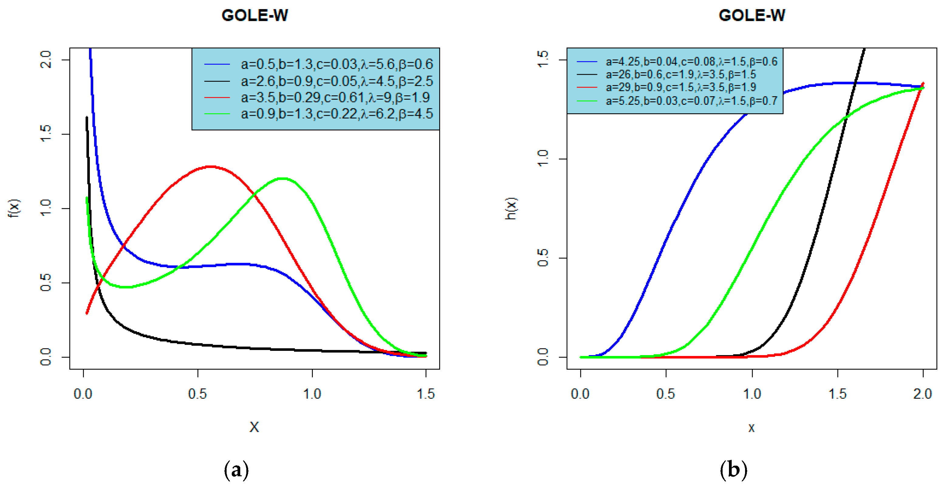
Consider the Weibull distribution with density and distribution functions $f\left(x;\lambda ,\beta \right)=\lambda \beta x^{\beta -1}{e}^{-\lambda x^{\beta }}$ and $F\left(x;\lambda ,\beta \right)=1-e^{-\lambda x^{\beta }}$, respectively, where $\lambda ,\beta >0$ and $x\ge 0$. Then, the GOLE-W distribution has (PDF) provided by

$$\begin{array}{ll}\hfill g\left(x;a,b,c,\lambda ,\beta \right)& =\left[\frac{c\lambda \beta x^{\beta -1}{e}^{-\lambda x^{\beta }}{\left(1-e^{-\lambda x^{\beta }}\right)}^{c-1}\left(a+\left(b-a\right){\left(1-e^{-\lambda x^{\beta }}\right)}^c\right)}{{\left(1-{\left(1-e^{-\lambda x^{\beta }}\right)}^c\right)}^3}\right]\\ & \times \exp \left[-\left(\frac{a{\left(1-e^{-\lambda x^{\beta }}\right)}^c}{1-{\left(1-e^{-\lambda x^{\beta }}\right)}^c}+\frac{b}{2}{\left(\frac{{\left(1-e^{-\lambda x^{\beta }}\right)}^c}{1-{\left(1-e^{-\lambda x^{\beta }}\right)}^c}\right)}^2\right)\right].\end{array}$$

Figure 1a show a wealth of possible shapes of the distribution once different choices of the parameters are made. For example, the shape can be U and inverted-U, right-skewed, reversed-J shape or symmetrical. Additionally, Figure 1b reveal that the HRF of the GOLE-W distribution can be increasing–constant, constant–monotone–increasing or monotone–increasing shapes.

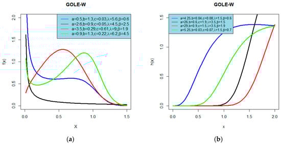
Figure 1. (a) Density function and (b) hazard rate plots of the GOLE-W distribution for different parameter values.

3.2. The Generalized Odd Linear Exponential-Exponential (GOLE-E) Distribution

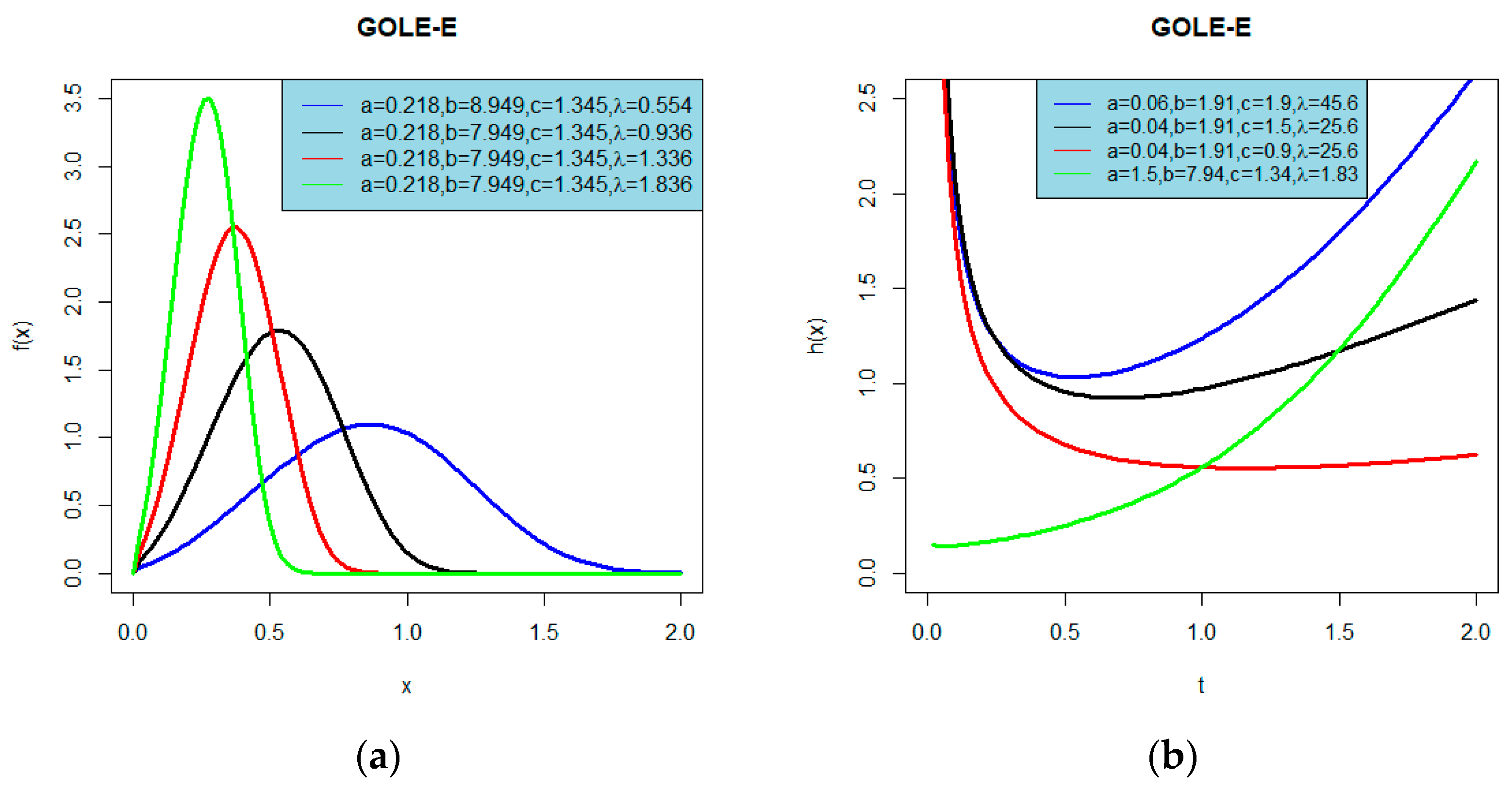
Consider the Exponential distribution with density and distribution functions $f\left(x;\lambda \right)=\lambda e^{-\lambda x}$ and $F\left(x;\lambda \right)=1-e^{-\lambda x}$, respectively, where $\lambda >0$ and $x\ge 0$. Then, the GOLE-E distribution has (PDF) provided by

$$g\left(x;a,b,c,\lambda \right)=\left[\frac{c\lambda e^{-\lambda x}{\left(1-e^{-\lambda x}\right)}^{c-1}\left(a+\left(b-a\right){\left(1-e^{-\lambda x}\right)}^c\right)}{{\left(1-{\left(1-e^{-\lambda x}\right)}^c\right)}^3}\right]\times \exp \left[-\left(\frac{a{\left(1-e^{-\lambda x}\right)}^c}{1-{\left(1-e^{-\lambda x}\right)}^c}+\frac{b}{2}{\left(\frac{{\left(1-e^{-\lambda x}\right)}^c}{1-{\left(1-e^{-\lambda x}\right)}^c}\right)}^2\right)\right].$$

Figure 2a show possible shapes of the GOLE-E distribution for different choices of the parameters. The shapes of pdf can be right-skewed, or symmetrical. Further, Figure 2b reveal that the HRF of the GOLE-E distribution can be decreasing–constant, monotone–increasing or bathtub shape. The PDF and HRF of the GOLE-W and GOLE-E distributions for some selected values of the parameters indicate the flexibility of the new family.

Figure 2. Plots of (a) density function and (b) hazard rate of the GOLE-E distribution for different parameter values.

4. Mathematical Properties of the GOLE-F Family

In this section, some mathematical properties of the GOLE-F family are obtained.

4.1. Asymptotic Behavior of GOLE-F Family

First of all, for the statements of the following results, we recall that $F\left(x\right)$ is the CDF of an absolutely continuous distribution with pdf $f\left(x\right)$.

Proposition 1.

The asymptotes corresponding to Equations (3)–(5) when$x\to -\infty$are provided by

$$G\left(x\right)~a F{\left(x\right)}^c,$$

(9)

$$g\left(x\right)~c a f\left(x\right)F{\left(x\right)}^{c-1},$$

(10)

$$h\left(x\right)~c a f\left(x\right)F{\left(x\right)}^{c-1}.$$

(11)

Proposition 2.

The asymptotes corresponding to Equations (3)–(5) when$x\to \infty$are provided by

$$1-G\left(x\right) ~ 1-e^{-\left(\frac{a}{1-F{\left(x\right)}^c }+\frac{b}{2}{\left\{\frac{1}{1-F{\left(x\right)}^c }\right\}}^2\right)},$$

(12)

$$g\left(x\right)~\frac{bcf\left(x\right)}{{\left(1-F{\left(x\right)}^c\right)}^3} e^{-\left(\frac{a}{1-F{\left(x\right)}^c }+\frac{b}{2}{\left\{\frac{1}{1-F{\left(x\right)}^c }\right\}}^2\right)}$$

(13)

$$h\left(x\right)~\frac{bcf\left(x\right)}{{\left(1-F{\left(x\right)}^c\right)}^3}.$$

(14)

For detail seeAppendix A.

4.2. Useful Expansions for CDF and PDF of the New Family

Using the power series for the exponential function and the generalized binomial expansion

$$e^{-z}={\displaystyle \sum }_{i=0}^{\infty }\frac{{\left(-1\right)}^i{z}^i}{i!},$$

and

$${\left(1-v\right)}^n={\displaystyle \sum }_{i=0}^{\infty }{\left(-1\right)}^i\left(\begin{array}{c}n\\ i\end{array}\right)v^i,$$

respectively, where $\left|v\right|<1$ and $n$ is any real number, we can rewrite the CDF of the GOLE-F family as follows:

$$G\left(x;a,b,c,\mathit{\varphi }\right)=1-{\displaystyle \sum }_{i=0}^{\infty }{\displaystyle \sum }_{j=0}^i{\displaystyle \sum }_{k=0}^{\infty }\frac{{\left(-1\right)}^i{b}^j{a}^i\left(\begin{array}{c}i\\ j\end{array}\right)\left(\begin{array}{c}i+j+k-1\\ k\end{array}\right)}{i!2^j}F{\left(x\right)}^{c\left(i+j+k\right)}.$$

(15)

Again, based on the binomial expansion, we find

$$F{\left(x\right)}^{c\left(i+j+k\right)}={\left(1-(1-F\left(x\right)\right)}^{c\left(i+j+k\right)}={\displaystyle \sum }_{m=0}^{\infty }{\displaystyle \sum }_{l=m}^{\infty }{\left(-1\right)}^{l+m}\left(\begin{array}{c}l\\ m\end{array}\right)\left(\begin{array}{c}c\left(i+j+k\right)\\ l\end{array}\right)F{\left(x\right)}^m.$$

(16)

From (15) and (16), we obtain

$$G\left(x;a,b,c,\mathit{\varphi }\right)=1-{\displaystyle \sum }_{m=0}^{\infty }{\omega }_{m}F{\left(x\right)}^m,$$

(17)

where

$${\omega }_m={\displaystyle \sum }_{l=m}^{\infty }{\displaystyle \sum }_{i=0}^{\infty }{\displaystyle \sum }_{j=0}^i{\displaystyle \sum }_{k=0}^{\infty }{\rho }_{i,j,k,l}\left(a,b,c\right),$$

and

$${\rho }_{i,j,k,l}\left(a,b,c\right)=\frac{{\left(-1\right)}^{i+l+m}{b}^j{a}^i\left(\begin{array}{c}i\\ j\end{array}\right)\left(\begin{array}{c}l\\ m\end{array}\right)\left(\begin{array}{c}i+j+k-1\\ k\end{array}\right)\left(\begin{array}{c}c\left(i+j+k\right)\\ l\end{array}\right)}{i!2^j}.$$

Now, we can write the CDF of the GOLE-F family in Equation (17), as

$$G\left(x;a,b,c,\mathit{\varphi }\right)={\displaystyle \sum }_{m=0}^{\infty }{\delta }_{m}F{\left(x\right)}^m,$$

(18)

where ${\delta }_0=1-{\omega }_0$, and ${\delta }_m=-{\omega }_m$ for $m=1,2,\dots$ By differentiating Equation (18), we obtain the expansion of the density function of the GOLE-F family as an infinite linear mixture of exp-F densities in the following form

$$g\left(x;a,b,c,\mathit{\varphi }\right)={\displaystyle \sum }_{m=0}^{\infty }{\delta }_{m+1}{\pi }_{m+1}\left(x\right),$$

(19)

where ${\pi }_{m+1}\left(x\right)=\left(m+1\right)f\left(x\right)F{\left(x\right)}^m$ is the exp-F density function with power parameter $\left(m+1\right)$. Now, if the random variable $Y_{m+1}$ has the density function ${\pi }_{m+1}\left(x\right)$, then many mathematical properties of the random variable $X,$ including the ordinary and incomplete moments and moment generating function can easily be obtained based on the exp-F distribution.

4.3. Moments

Suppose that the random variable $Y_{m+1}$ has the density function ${\pi }_{m+1}\left(x\right)$ in (19), then the nth moment of the random variable $X$ can be obtained from

$${\mu }_n^{\prime }=E\left(X^n\right)={\displaystyle \sum }_{m=0}^{\infty }{\delta }_{m+1}E\left(Y_{m+1}^n\right).$$

(20)

A second alternative formula for ${\mu }_n^{\prime }$in terms of the baseline qf. $Q_F\left(u\right)$ can be obtained as

$${\mu }_n^{\prime }={\displaystyle \sum }_{m=0}^{\infty }{\delta }_{m+1}\left(m+1\right){{\displaystyle \int }}_0^1{Q}_F{\left(u\right)}^n{u}^{m}du,$$

(21)

where $Q_F\left(u\right)=F^{-1}\left(u\right)$ is the qf of the parent distribution and $u\in \left(0,1\right).$

The incomplete moments have an important role in measuring inequality, for example, income quantiles, the mean deviations and Lorenz and Bonferroni curves. The nth incomplete moment of $X$ is provided by

$${\eta }_n\left(z\right)={\displaystyle \sum }_{m=0}^{\infty }{\delta }_{m+1}\left(m+1\right){{\displaystyle \int }}_0^{F\left(z\right)}{Q}_F{\left(u\right)}^n{u}^{m}du.$$

(22)

The last integral can be computed analytically or numerically for most baseline distributions. Bonferroni and Lorenz curves have applications in many different areas such as economics to study income and poverty, reliability, demography, insurance and medicine. For a random variable $X,$ the Bonferroni and Lorenz curves are defined by $B\left(p\right)={\eta }_1\left(q\right)/pE\left(X\right)$ and $L\left(p\right)={\eta }_1\left(q\right)/E\left(X\right)$, respectively, where $p$ is a given probability, $q=Q\left(p\right)$ and ${\eta }_1\left(q\right)$ is the first incomplete moment that can be calculated from the above Equation with $r=1$ at $q$. Table 1 display the mean, variance, skewness and kurtosis of the GOLE-E distribution for some choices values of the parameters. We note from Table 1 that the skewness of the GOLE-E distribution is always positive, whereas the kurtosis of the GOLE-E distribution varies only in the interval (1.0571, 2.6112).

Table 1. Mean, variance, skewness and kurtosis of the GOLE-E distribution with different values of $a$, $b$, $c$ and $\lambda =1$.

a	b	c	Mean	Variance	Skewness	Kurtosis
0.5	0.5	1	0.6704	0.1330	1.2979	1.8368
		2	1.1667	0.2186	1.1776	1.4755
		5	1.9517	0.3004	1.0960	1.2512
		10	2.5987	0.3351	1.0635	1.1656
		20	3.2683	0.3541	1.0440	1.1146
		50	4.1704	0.3660	1.0288	1.0753
		100	4.8587	0.3701	1.0218	1.0571
1	1	1	0.4614	0.0824	1.3869	2.1392
		2	0.8995	0.1587	1.2180	1.5987
		5	1.6411	0.2408	1.1103	1.2923
		10	2.2721	0.2776	1.0699	1.1839
		20	2.9334	0.2982	1.0467	1.1226
		50	3.8303	0.3114	1.0294	1.0774
		100	4.5169	0.3159	1.0218	1.0574
2	1.5	1	0.3091	0.0488	1.5119	2.6112
		2	0.6860	0.1130	1.2703	1.7688
		5	1.3790	0.1919	1.1269	1.3424
		10	1.9914	0.2297	1.0768	1.2044
		20	2.6430	0.2514	1.0494	1.1308
		50	3.5339	0.2654	1.0299	1.0793
		100	4.2185	0.2702	1.0217	1.0574

4.4. Generating Function

Here, we provide three formulae for the mgf $M\left(t\right)=E\left(e^{tX}\right)$ of the random variable $X$. The first one is provided by

$$M\left(t\right)={\displaystyle \sum }_{n=0}^{\infty }\frac{t^n}{n!}{\mu }_n^{\prime },$$

(23)

where ${\mu }_n^{\prime }$is the nth moment of the random variable $X$. A second formula for $M\left(t\right)$ comes from (19) as

$$M\left(t\right)={\displaystyle \sum }_{m=0}^{\infty }{\delta }_{m+1}{M}_{m+1}\left(t\right),$$

(24)

where $M_{m+1}\left(t\right)$is the mgf of the random variable $Y_{m+1}~$exp-F ($m+1$). A third formula for $M\left(t\right)$ can also be derived based on (19) in terms of the baseline qf. $Q_F\left(u\right)$ as

$$M\left(t\right)={\displaystyle \sum }_{m=0}^{\infty }{\delta }_{m+1}\left(m+1\right){{\displaystyle \int }}_0^1\exp \left(t{Q}_F\left(u\right)\right)u^{m}du,$$

(25)

where $Q_F\left(u\right)=F^{-1}\left(u\right)$ is the qf of the baseline distribution and $u\in \left(0,1\right).$

4.5. Mean Deviations

The amount of scattering in a population is evidently measured to some extent by the totality of deviations from the mean and median. These are known as the mean deviation about the mean and the mean deviation about the median. These measures can be calculated using the following relationships:

${\delta }_1\left(X\right)=2\mu G\left(\mu \right)-2{\int }_{-\infty }^{\mu }xg\left(x\right)dx$ and ${\delta }_2\left(X\right)=\mu -2{\int }_{-\infty }^{M}xg\left(x\right)dx,$ respectively, where $\mu =E\left(X\right)$ and $M=Q\left(\frac{1}{2}\right)$.

4.6. Order Statistics

Let $X_1,X_2,\dots ,X_n$be a random sample from the GOLE-F family with CDF and PDF defined in Equations (3) and (4), respectively. Suppose $X_{1:n},X_{2:n},\dots ,X_{n:n}$ denote the order statistics obtained from this sample and $X_{r:n}$ is the $i\mathrm{th}$ order statistic, then the density function of the $r$th order statistic is provided by

$$g_{r:n}\left(x\right)=\frac{n!}{\left(r-1\right)!\left(n-r\right)!}{\displaystyle \sum }_{s=0}^{n-r}{\left(-1\right)}^s\left(\begin{array}{c}n-r\\ s\end{array}\right)g\left(x\right)G{\left(x\right)}^{r+s-1}.$$

(26)

From (17), we determine

$$G{\left(x\right)}^{r+s-1}={\left[{\displaystyle \sum }_{m=0}^{\infty }{\delta }_{m}F{\left(x\right)}^m\right]}^{r+s-1}={\displaystyle \sum }_{m=0}^{\infty }{d}_{r+s-1,m}F{\left(x\right)}^m,$$

(27)

where

$d_{r+s-1,0}={\delta }_0^{r+s-1}$ and $d_{r+s-1,m}={\left(m{\delta }_0\right)}^{-1}{\displaystyle \sum }_{q=1}^m\left[q\left(r+s\right)-m\right]{\delta }_q{d}_{r+s-1,m-q}.$

By replacing $t$instead of $m$ in Equation (19), we obtain

$$g\left(x\right)={\displaystyle \sum }_{t=0}^{\infty }{\delta }_{t+1}\left(t+1\right)f\left(x\right)F{\left(x\right)}^t.$$

(28)

By substituting (26) in (27) and (28), we determine the PDF of the $r\mathrm{th}$ order statistic $X_{r:n}$ as

$$g_{r:n}\left(x\right)={\displaystyle \sum }_{t,m=0}^{\infty }{\pi }_{t,m}{h}_{t+m+1}\left(x\right),$$

(29)

where $h_{t+m+1}\left(x\right)$ denotes the PDF of exp-F distribution with power parameter $\left(t+m+1\right)$, and

$${\pi }_{t,m}={\displaystyle \sum }_{s=0}^{n-r}\frac{{\left(-1\right)}^s\left(\begin{array}{c}n-r\\ s\end{array}\right)n!{\delta }_{t+1}\left(t+1\right)d_{r+s-1,m}}{\left(r-1\right)!\left(n-r\right)!\left(t+m+1\right)} .$$

Based on Equation (29), several mathematical properties of these order statistics such as ordinary and incomplete moments, factorial moments, moment generating function, mean deviations and several others, can be obtained.

4.7. Stochastic Orderings

Stochastic orders and inequalities are used in many different areas of probability and statistics. Such areas include reliability theory, survival analysis, economics, insurance, actuarial science, queuing theory, biology, operations research, management science, etc. For more detail regarding stochastic ordering, see (Shaked et al., 1994 [15]). Given two random variables $X$ and $Y$, we say that $X$ is smaller than $Y$ in the:

• usual stochastic order, denoted by $X{\le }_{st}Y$, if $G_X\left(x\right)\ge G_Y\left(x\right)$, for all $x$;
• hazard rate order, denoted by $X{\le }_{hr}Y$, if $h_X\left(x\right)\ge h_Y\left(x\right)$, for all $x$;
• reversed hazard rate order, denoted by $X{\le }_{rh}Y$, if $G_X\left(x\right)/G_Y\left(x\right),$ is decreases in $x$;
• mean residual life order, denoted by $X{\le }_{mrl}Y$, if $m_X\left(x\right)\le m_Y\left(x\right)$, for all $x$;
• likelihood ratio order, denoted by $X{\le }_{lr}Y$, if $g_X\left(x\right)/g_Y\left(x\right),$ is decreases in $x$.

For all the previous orders, we determine the following chains of implications:

$$X{\le }_{lr}Y\Rightarrow X{\le }_{hr}Y\Rightarrow X{\le }_{st}Y$$

and

$$X{\le }_{lr}Y\Rightarrow X{\le }_{rh}Y\Rightarrow X{\le }_{st}Y,$$

also

$$X{\le }_{hr}Y\Rightarrow X{\le }_{mrl}Y.$$

For the proposed GOLE-F family, the following theorem provides the stochastic comparison results with respect to the above orderings.

Theorem 1.

Let $X~GOLE\left(a_1,b_1, c_1,\mathit{\varphi }\right)$and $Y~GOLE\left(a_2,b_2, c_2,\mathit{\varphi }\right)$. If $a_1\ge a_2$. and $b_1\ge b_2$and $c_1\le c_2$, then $X{\le }_{st}Y$.

Proof. 

If $c_1\le c_2$, then

$$\frac{F{\left(x\right)}^{ c_1}}{1-F{\left(x\right)}^{ c_1}}\ge \frac{F{\left(x\right)}^{ c_2}}{1-F{\left(x\right)}^{ c_2}}.$$

(30)

Hence, if $a_1\ge a_2$ and $b_1\ge b_2$, then

$$\frac{a_{1}F{\left(x\right)}^{c_1}}{1-F{\left(x\right)}^{c_1}}+\frac{b_1}{2}{\left(\frac{F{\left(x\right)}^{c_1}}{1-F{\left(x\right)}^{c_1}}\right)}^2\ge \frac{a_{2}F{\left(x\right)}^{c_2}}{1-F{\left(x\right)}^{c_2}}+\frac{b_2}{2}{\left(\frac{F{\left(x\right)}^{c_2}}{1-F{\left(x\right)}^{c_2}}\right)}^2.$$

(31)

Therefore,

$$\left[-\left(\frac{a_{1}F{\left(x\right)}^{c_1}}{1-F{\left(x\right)}^{c_1}}+\frac{b_1}{2}{\left(\frac{F{\left(x\right)}^{c_1}}{1-F{\left(x\right)}^{c_1}}\right)}^2\right)\right]\le \left[-\left(\frac{a_{2}F{\left(x\right)}^{c_2}}{1-F{\left(x\right)}^{c_2}}+\frac{b_2}{2}{\left(\frac{F{\left(x\right)}^{c_2}}{1-F{\left(x\right)}^{c_2}}\right)}^2\right)\right].$$

(32)

Thus,

$$\begin{array}{l}1-\exp \left[-\left(\frac{a_{1}F{\left(x\right)}^{c_1}}{1-F{\left(x\right)}^{c_1}}+\frac{b_1}{2}{\left(\frac{F{\left(x\right)}^{c_1}}{1-F{\left(x\right)}^{c_1}}\right)}^2\right)\right]\\ \ge 1-\exp \left[-\left(\frac{a_{2}F{\left(x\right)}^{c_2}}{1-F{\left(x\right)}^{c_2}}+\frac{b_2}{2}{\left(\frac{F{\left(x\right)}^{c_2}}{1-F{\left(x\right)}^{c_2}}\right)}^2\right)\right].\end{array}$$

(33)

That means $G_X\left(x\right)\ge G_Y\left(x\right)$ and $X{\le }_{st}Y$. □

Theorem 2.

Let $X~GOLE\left(a_1,b_1, c,\mathit{\varphi }\right)$ and $Y~GOLE\left(a_2,b_2, c,\mathit{\varphi }\right)$. If $a_1>a_2$ and $b_1=b_2$, then $X{\le }_{lr}Y$.

Proof. 

We determine

$$\frac{g_X\left(x\right)}{g_Y\left(x\right)}=\frac{\left[\left(a_1+\left(b_1-a_1\right)F{\left(x\right)}^c\right)\right]\times \exp \left[-\left(\frac{a_{1}F{\left(x\right)}^c}{1-F{\left(x\right)}^c}+\frac{b_1}{2}{\left(\frac{F{\left(x\right)}^c}{1-F{\left(x\right)}^c}\right)}^2\right)\right]}{\left[\left(a_2+\left(b_2-a_2\right)F{\left(x\right)}^c\right)\right]\times \exp \left[-\left(\frac{a_{2}F{\left(x\right)}^c}{1-F{\left(x\right)}^c}+\frac{b_2}{2}{\left(\frac{F{\left(x\right)}^c}{1-F{\left(x\right)}^c}\right)}^2\right)\right]}.$$

(34)

Thus,

$$\begin{array}{ll}\hfill \log \left(\frac{g_X\left(x\right)}{g_Y\left(x\right)}\right)=\log & \left[\left(a_1+\left(b_1-a_1\right)F{\left(x\right)}^c\right)\right]-\left(\frac{a_{1}F{\left(x\right)}^c}{1-F{\left(x\right)}^c}+\frac{b_1}{2}{\left(\frac{F{\left(x\right)}^c}{1-F{\left(x\right)}^c}\right)}^2\right)\\ & -\log \left[\left(a_2+\left(b_2-a_2\right)F{\left(x\right)}^c\right)\right]+\left(\frac{a_{2}F{\left(x\right)}^c}{1-F{\left(x\right)}^c}+\frac{b_2}{2}{\left(\frac{F{\left(x\right)}^c}{1-F{\left(x\right)}^c}\right)}^2\right).\end{array}$$

(35)

By differentiating the last Equation and after some simplifications, we obtain

$$\begin{array}{ll}\hfill \frac{d}{dx}\left(\log \left(\frac{g_X\left(x\right)}{g_Y\left(x\right)}\right)\right)& \\ & =\frac{\left(a_2{b}_1-a_1{b}_2\right)cf\left(x\right)F{(x)}^{c-1}}{\left(a_1+\left(b_1-a_1\right)F{(x)}^c\right)\left(a_2+\left(b_2-a_2\right)F{(x)}^c\right)}+\frac{\left(a_2-a_1\right)cf\left(x\right)F{(x)}^{c-1}}{{\left(1-F{(x)}^c\right)}^2}+\frac{\left(b_2-b_1\right)cf\left(x\right)F{(x)}^{2c-1}}{{\left(1-F{(x)}^c\right)}^3}.\end{array}$$

(36)

Now, if $a_1>a_2$ and $b_1=b_2$, then $\frac{d}{dx}\left[\log \left(\frac{g_X\left(x\right)}{g_Y\left(x\right)}\right)\right]<0$, and hence $g_X\left(x\right)/g_Y\left(x\right)$ is decreases in $x$. This implies that$X{\le }_{lr}Y$. □

4.8. Stress-Strength Model

The stress–strength model defines the life of an element which has a random strength $Y$ that is subjected to an accidental stress $X$. The component fails at the instant that the stress applied to it exceeds the strength, and the component will function suitably whenever $X<Y$. Hence, $R=P(X<Y)$ is a measure of component reliability (Kotz et al., 2003 [16]). It has many applications, especially in reliability engineering. We derive the reliability R when Y and X are two independent continuous random variables from the GOLE-F $\left(a_1,b_1,c_1,{\mathit{\varphi }}_1\right)$ and GOLE-F $\left(a_2,b_2,c_2,{\mathit{\varphi }}_2\right)$ distributions, respectively. The reliability is defined by

$$R={{\displaystyle \int }}_0^{\infty }{g}_Y\left(x\right)G_X\left(x\right)dx.$$

(37)

Using the PDF in (19) and the CDF in (18), we obtain

$$R={\displaystyle \sum }_{m,t=0}^{\infty }{\delta }_{m+1}{\delta }_t{R}_{m+1,t },$$

(38)

where

$R_{m+1,t}={\int }_0^{\infty }{\pi }_{m+1}\left(x,{\mathit{\varphi }}_1\right){\Pi }_t\left(x,{\mathit{\varphi }}_2\right)dx,$ and

${\pi }_{m+1}\left(x,{\mathit{\varphi }}_1\right)=\left(m+1\right)f\left(x,{\mathit{\varphi }}_1\right)F{\left(x,{\mathit{\varphi }}_1\right)}^m$, ${\Pi }_t\left(x,{\mathit{\varphi }}_2\right)=F{\left(x,{\mathit{\varphi }}_2\right)}^t$.

The constants ${\delta }_t,{\delta }_{m+1}$ are defined as:

$${\delta }_t={\displaystyle \sum }_{l=t}^{\infty }{\displaystyle \sum }_{i=0}^{\infty }{\displaystyle \sum }_{j=0}^i{\displaystyle \sum }_{k=0}^{\infty }\frac{{\left(-1\right)}^{i+l+t+1}{b}_2^j{a}_2^i\left(\begin{array}{c}i\\ j\end{array}\right)\left(\begin{array}{c}l\\ t\end{array}\right)\left(\begin{array}{c}i+j+k-1\\ k\end{array}\right)\left(\begin{array}{c}{c}_2\left(i+j+k\right)\\ l\end{array}\right)}{i!2^j},$$

for $t\ge 1$. For $t=0$, then

$${\delta }_0=1-{\displaystyle \sum }_{l=0}^{\infty }{\displaystyle \sum }_{i=0}^{\infty }{\displaystyle \sum }_{j=0}^i{\displaystyle \sum }_{k=0}^{\infty }\frac{{\left(-1\right)}^{i+l+m}{b}_2^j{a}_2^i\left(\begin{array}{c}i\\ j\end{array}\right)\left(\begin{array}{c}i+j+k-1\\ k\end{array}\right)\left(\begin{array}{c}{c}_2\left(i+j+k\right)\\ l\end{array}\right)}{i!2^j},$$

and

$${\delta }_{m+1}={\displaystyle \sum }_{l=m+1}^{\infty }{\displaystyle \sum }_{i=0}^{\infty }{\displaystyle \sum }_{j=0}^i{\displaystyle \sum }_{k=0}^{\infty }\frac{{\left(-1\right)}^{i+l+m+2}{b}_1^j{a}_1^i\left(\begin{array}{c}i\\ j\end{array}\right)\left(\begin{array}{c}l\\ m+1\end{array}\right)\left(\begin{array}{c}i+j+k-1\\ k\end{array}\right)\left(\begin{array}{c}{c}_1\left(i+j+k\right)\\ l\end{array}\right)}{i!2^j},$$

for $m\ge 0$.

If ${\mathit{\varphi }}_1={\mathit{\varphi }}_2$, then the model reduces to

$$R={\displaystyle \sum }_{m,t=0}^{\infty }\frac{{\delta }_{m+1}{\delta }_t\left(m+1\right)}{m+t+1}.$$

(39)

5. Estimation and Simulation

5.1. Estimation of the Parameters

Here, we find the maximum likelihood estimates (MLEs) of the parameters of the new family of distributions from complete samples only. Let $x_1,x_2,\dots ,x_n$ be observed values from the $\mathrm{GOLE}-\mathrm{F}$ family with parameters $a,b,c$and $\mathit{\varphi }$. Let $\mathit{\xi }={\left(a,b,c,\mathit{\varphi }\right)}^T$ be the parameters vector. The total log-likelihood function for $\mathit{\xi }$ is obtained by

$$\begin{array}{ll}\hfill l\left(\mathit{\xi }\right)=n \log c& +{\displaystyle {\displaystyle \sum }_{i=1}^n}\log f\left(x_i;\mathit{\varphi }\right)+\left(c-1\right){\displaystyle {\displaystyle \sum }_{i=1}^n}\log F\left(x_i;\mathit{\varphi }\right)+{\displaystyle {\displaystyle \sum }_{i=1}^n}\log \left(a+\left(b-a\right)F{\left(x_i;\mathit{\varphi }\right)}^c\right)\\ & -3{\displaystyle {\displaystyle \sum }_{i=1}^n}\log \left(1-F{\left(x_i;\mathit{\varphi }\right)}^c\right)-a{\displaystyle {\displaystyle \sum }_{i=1}^n}H\left(x_i,\mathit{\varphi }\right)-\frac{b}{2}{\displaystyle {\displaystyle \sum }_{i=1}^n}H{\left( x_i,\mathit{\varphi }\right)}^2,\end{array}$$

(40)

where $H\left(x_i,\mathit{\varphi }\right)=\frac{F{\left(x_i;\mathit{\varphi }\right)}^c}{1-F{\left(x_i;\mathit{\varphi }\right)}^c}$ and $H{\left(x_i,\mathit{\varphi }\right)}^2={\left(\frac{F{\left(x_i;\mathit{\varphi }\right)}^c}{1-F{\left(x_i;\mathit{\varphi }\right)}^c}\right)}^2$.

The components of the score vector $U\left(\mathit{\xi }\right)$are obtained by

$$U_a={\displaystyle \sum }_{i=1}^n\frac{1-F{\left(x_i;\mathit{\varphi }\right)}^c}{a+\left(b-a\right)F{\left(x_i;\mathit{\varphi }\right)}^c}-{\displaystyle \sum }_{i=1}^{n}H\left(x_i,\mathit{\varphi }\right),$$

(41)

$$U_b={\displaystyle \sum }_{i=1}^n\frac{F{\left(x_i;\mathit{\varphi }\right)}^c}{a+\left(b-a\right)F{\left(x_i;\mathit{\varphi }\right)}^c}-\frac{1}{2}{\displaystyle \sum }_{i=1}^{n}H{\left( x_i,\mathit{\varphi }\right)}^2,$$

(42)

$$\begin{array}{c}{U}_c=\frac{n}{c}+{\displaystyle {\displaystyle \sum }_{i=1}^n}\log F\left(x_i;\mathit{\varphi }\right)+{\displaystyle {\displaystyle \sum }_{i=1}^n}\frac{\left(b-a\right)F{\left(x_i;\mathit{\varphi }\right)}^c\log F\left(x_i;\mathit{\varphi }\right)}{a+\left(b-a\right)F{\left(x_i;\mathit{\varphi }\right)}^c}+3{\displaystyle {\displaystyle \sum }_{i=1}^n}\frac{F{\left(x_i;\mathit{\varphi }\right)}^c\log F\left(x_i;\mathit{\varphi }\right)}{1-F{\left(x_i;\mathit{\varphi }\right)}^c}\\ -a{\displaystyle {\displaystyle \sum }_{i=1}^n}\frac{F{\left(x_i;\mathit{\varphi }\right)}^c\log F\left(x_i;\mathit{\varphi }\right)}{{\left(1-F{\left(x_i;\mathit{\varphi }\right)}^c\right)}^2}-b{\displaystyle {\displaystyle \sum }_{i=1}^n}\frac{F{\left(x_i;\mathit{\varphi }\right)}^{2c}\log F\left(x_i;\mathit{\varphi }\right)}{{\left(1-F{\left(x_i;\mathit{\varphi }\right)}^c\right)}^3},\end{array}$$

(43)

and

$$\begin{array}{ll}\hfill U_{{\mathit{\varphi }}_k}={\displaystyle {\displaystyle \sum }_{i=1}^n}\frac{\frac{\partial f\left(x_i;\mathit{\varphi }\right)}{\partial {\mathit{\varphi }}_k}}{f\left(x_i;\mathit{\varphi }\right)}& +\left(c-1\right){\displaystyle {\displaystyle \sum }_{i=1}^n}\frac{\frac{\partial F\left(x_i;\mathit{\varphi }\right)}{\partial {\mathit{\varphi }}_k}}{F\left(x_i;\mathit{\varphi }\right)}+{\displaystyle {\displaystyle \sum }_{i=1}^n} \frac{c\left(b-a\right)F{\left(x_i;\mathit{\varphi }\right)}^{c-1}\frac{\partial F\left(x_i;\mathit{\varphi }\right)}{\partial {\mathit{\varphi }}_k}}{a+\left(b-a\right)F{\left(x_i;\mathit{\varphi }\right)}^c}\\ & +3{\displaystyle {\displaystyle \sum }_{i=1}^n}\frac{cF{\left(x_i;\mathit{\varphi }\right)}^{c-1}\frac{\partial F\left(x_i;\mathit{\varphi }\right)}{\partial {\mathit{\varphi }}_k}}{1-F{\left(x_i;\mathit{\varphi }\right)}^c}-a{\displaystyle {\displaystyle \sum }_{i=1}^n}\frac{\partial H\left( x_i,\mathit{\varphi }\right)}{\partial {\mathit{\varphi }}_k}-b{\displaystyle {\displaystyle \sum }_{i=1}^n}H\left( x_i,\mathit{\varphi }\right)\frac{\partial H\left( x_i,\mathit{\varphi }\right)}{\partial {\mathit{\varphi }}_k}\end{array}$$

(44)

Setting $U_a,U_b,U_c$ and $U_{\mathit{\varphi }}$ equal to zero, and solving the equations simultaneously, yields the MLE $\widehat{\mathit{\xi }}={\left(\widehat{a},\widehat{b},\widehat{c},\widehat{\mathit{\varphi }}\right)}^T$ of $\mathit{\xi }={\left(a,b,c,\mathit{\varphi }\right)}^T$. These equations cannot be solved analytically, and statistical software can be used to solve them numerically using iterative methods such as the Newton–Raphson type algorithms.

5.2. Simulation Study

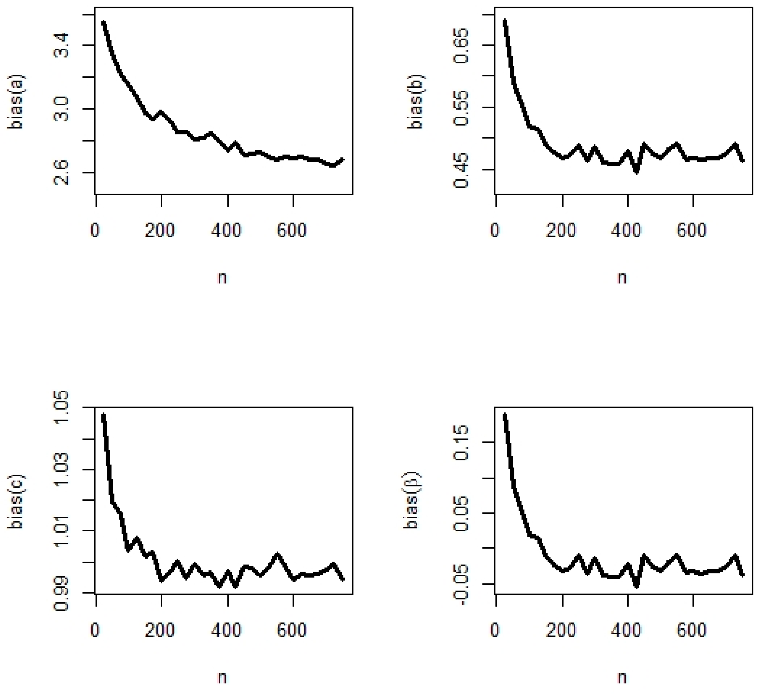
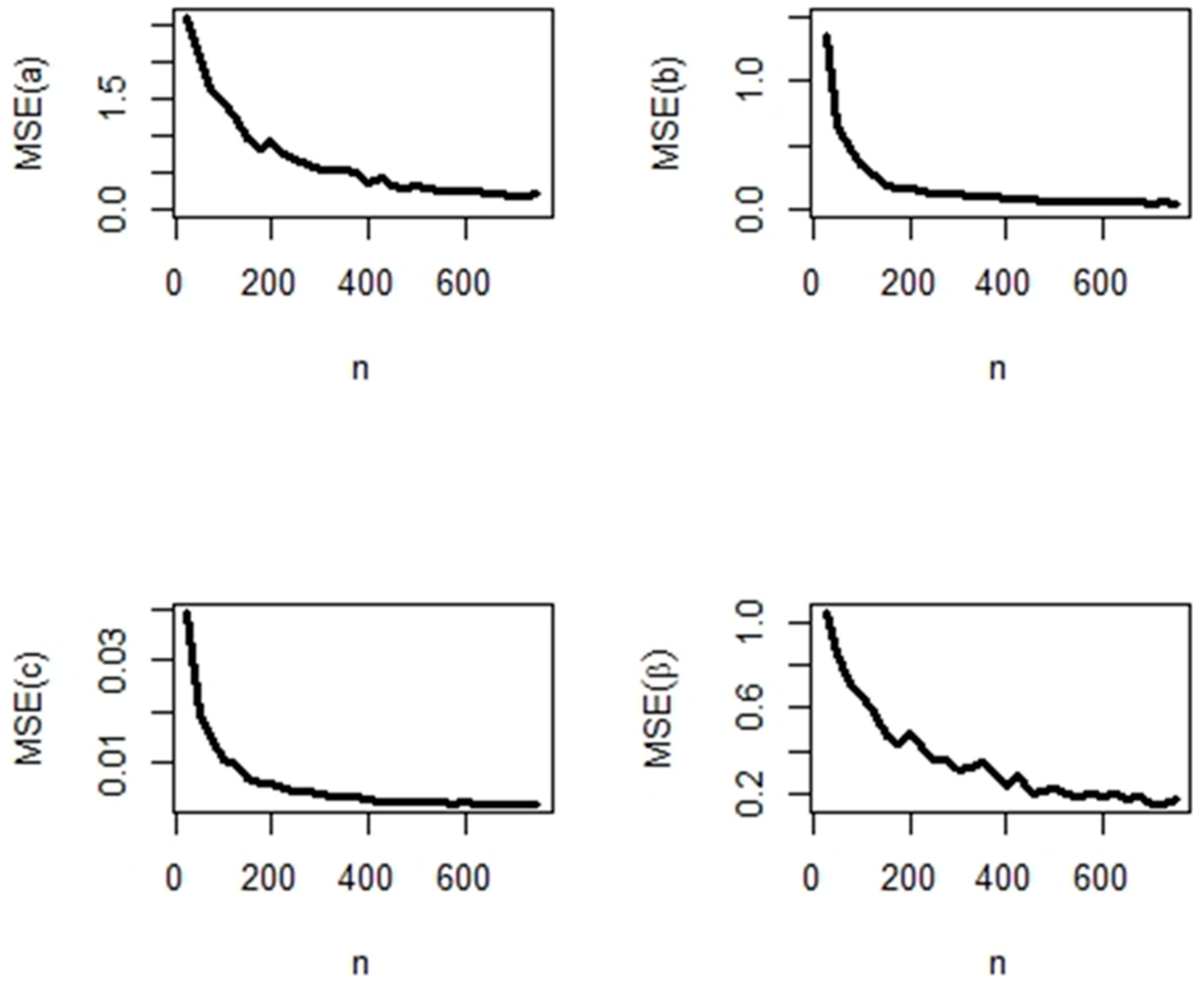
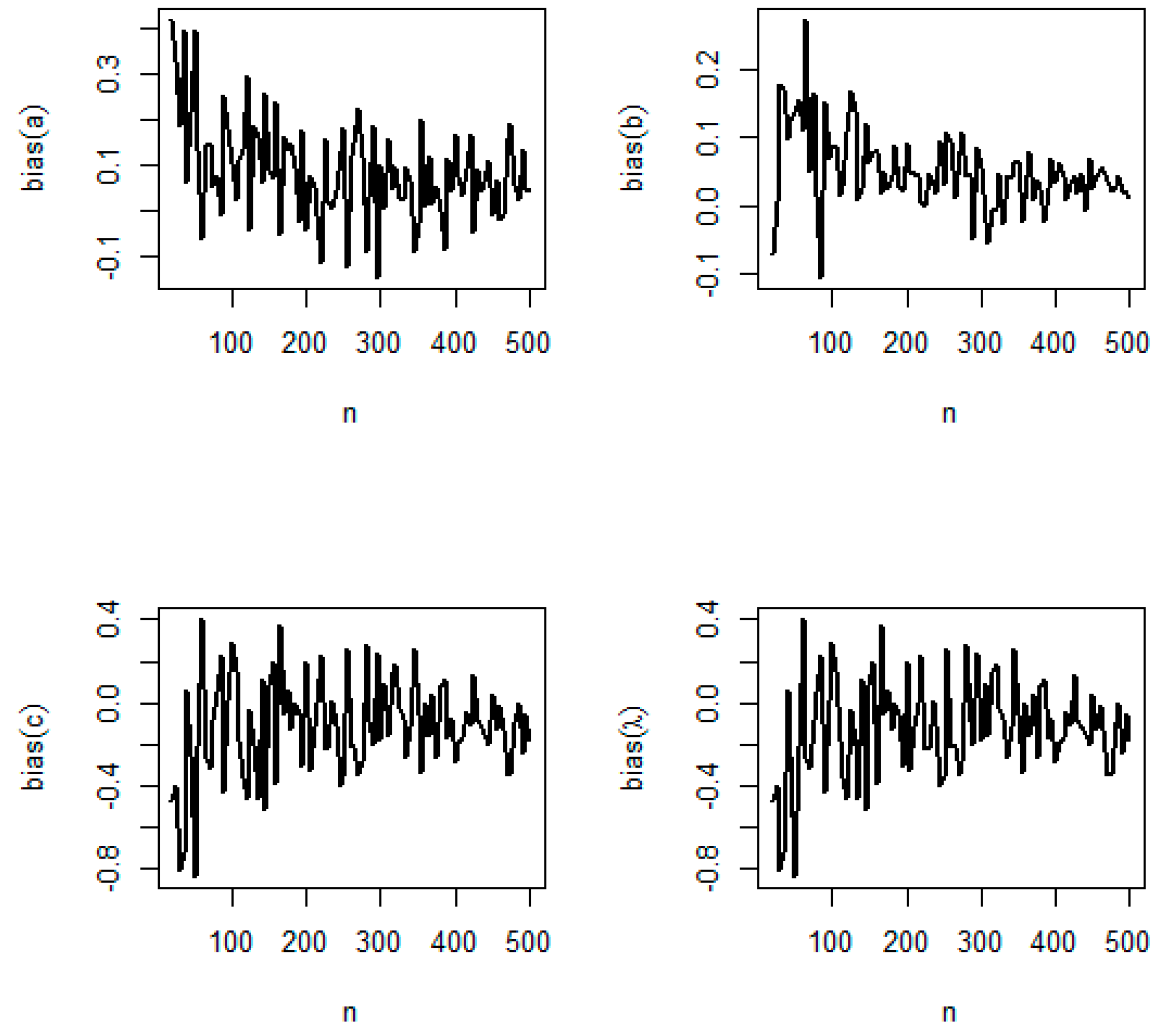
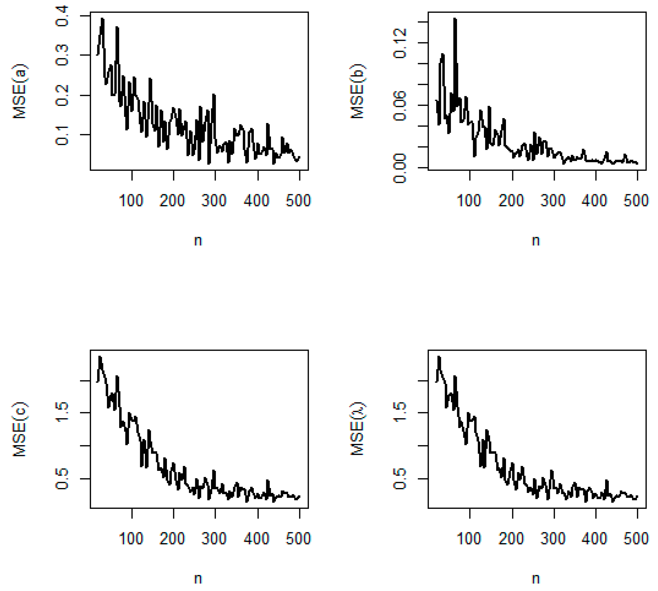
In this section, a graphical Monte Carlo simulation study is conducted to compare the performance of the different estimators of the unknown parameters for the GOLE-E ($a,b,c,\lambda$) distribution. All the computations in this section are conducted using the R program. We generate N = 1000 samples of size n = 20, 25, …, 500 from the GOLE-W and GOLE-E distributions. The true parameter values for GOLE-W ($\lambda =1$) are $a=1.8,b=0.5,c=1.7$ and $\beta =2.8,$ and those for GOLE-E are $a=2,b=1.5,c=2$ and $\lambda =2.5$, respectively. We also calculate the bias and mean square error (MSE) of the MLEs empirically. The bias and MSE are computed by

$${\widehat{Bias}}_h=\frac{1}{N}{\displaystyle \sum }_{i=1}^N\left({\widehat{h}}_i-h\right), {\widehat{MSE}}_h=\frac{1}{N}{\displaystyle \sum }_{i=1}^N{\left({\widehat{h}}_i-h\right)}^2.$$

For h = $a,b,c,\lambda ,$ respectively.

We provide the results of this simulation study in Figure 3, Figure 4, Figure 5 and Figure 6. From these figures, we can perceive that when the sample size increases, the empirical biases and MSEs approach zero in all cases for the two models.

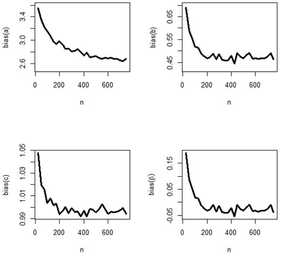
Figure 3. The biases of the estimates of parameters of the GOLE-W distribution.

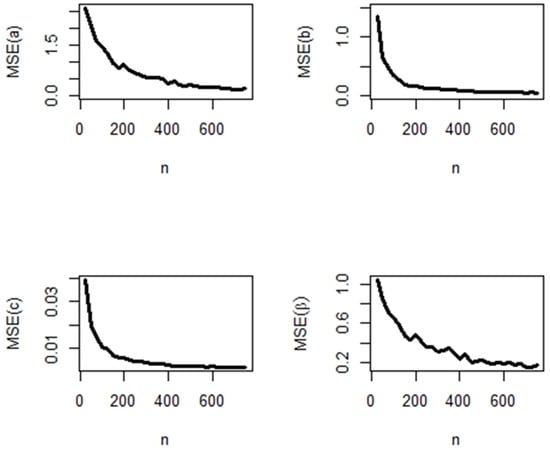
Figure 4. The MSEs of the estimates of parameters of the GOLE-W distribution.

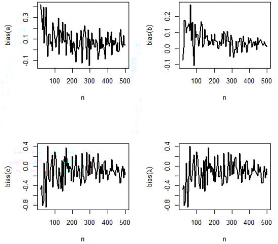
Figure 5. The biases of the estimates of parameters of the GOLE-E distribution.

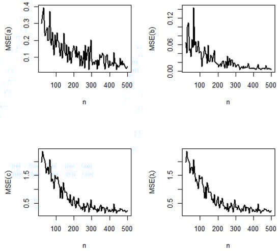
Figure 6. The MSE of the estimates of parameters of the GOLE-E distribution.

6. Applications on Real-Life Data Sets

In this section, we illustrate the suitability of the proposed family by fitting two real data sets on the special models viz-a-viz $\mathrm{GOLE}-\mathrm{W}\left(a,b,c,\lambda ,\beta \right)$ and $\mathrm{GOLE}-\mathrm{E} \left(a,b,c,\lambda \right)$, arising due to this family with PDF mentioned in Section 3.1 and Section 3.2, respectively. The comparison is conducted with some of the existing models via numerical maximizations of log-likelihood functions using the method of a limited memory quasi-Newton code for bound–constrained maximization (L-BFGS-B). We determine the log-likelihood function adjudicated at the MLEs by estimating the parameters.

Data I: The first data set is related to the measurements of nicotine levels in 346 cigarettes. [https://arxiv.org/ftp/arxiv/papers/1509/1509.08108.pdf, accessed on 19 May 2022]. Data II: The second data set consists of 74 observations of gauge lengths of 20 mm of single carbon fibers pertaining to failure stresses. (Kundu and Raqab, 2009 [17]). The descriptive statistics related to this data sets are given in Table 2.

Table 2. Descriptive Statistics for the data set I and data set II.

Data Sets	Min.	Mean	Median	S.D.	Skewness	Kurtosis	1st Q.	3rd Q.	Max.
I	0.10	0.85	0.90	0.33	0.17	0.29	0.60	1.10	2.00
II	1.312	2.477	2.513	0.487	−0.151	−0.127	2.150	2.816	3.5

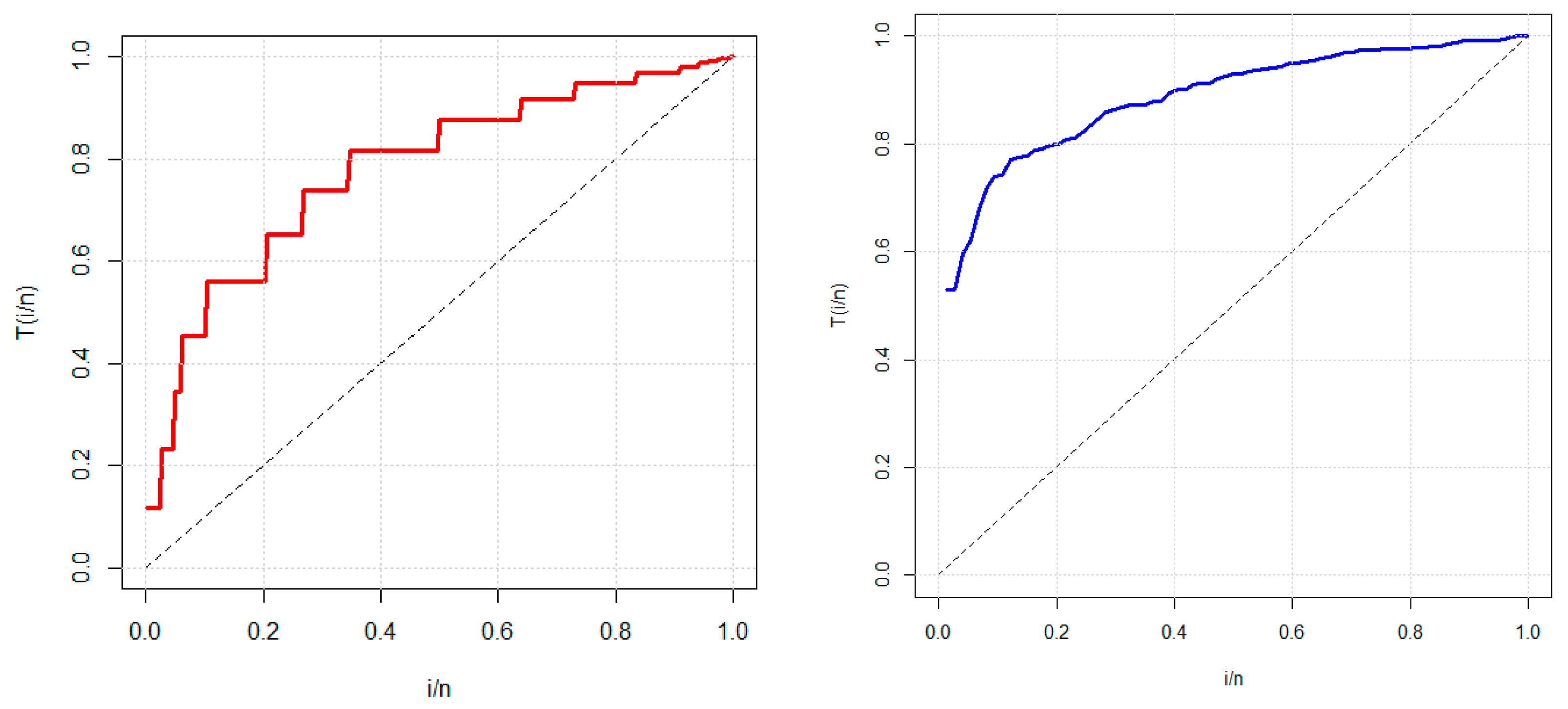
The total time on test (TTT) plot proposed by Aarset (1987) [18] is a technique to extract information about the shape of the hazard function. This is drawn by plotting $T\left(i/n\right)=\{(\sum _{r=1}^i{y}_{\left(r\right)})+(n-i)y_{(i)}\}/\sum _{r=1}^n{y}_{\left(r\right)}$, where $i=1,2,\dots ,n$ and $y_{\left(r\right)}$ where $r=1,2,\dots ,n$ is the order statistics of the sample against $\left(i/n\right)$. The constant hazard plot is a straight diagonal, while for decreasing (increasing) hazards, it is convex (concave), respectively. The TTT plots for the data sets in Figure 7 indicate that the data sets have an increasing hazard rate.

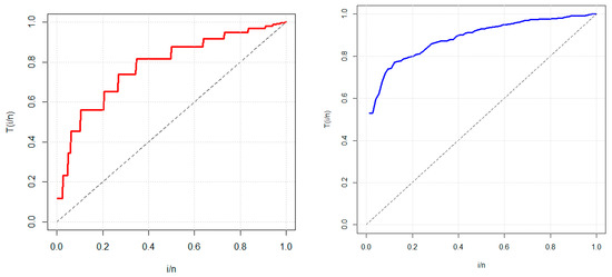
Figure 7. TTT plots of the data set I and II.

The best model is chosen on the basis of information criteria such as AIC (Akaike Information Criterion), CAIC (Consistent Akaike Information Criterion), BIC (Bayesian Information Criterion) and HQIC (Hannan–Quinn Information Criterion) with the goodness of fit measures as A* (Anderson–Darling criterion), W* (Cramér–von Mises criterion) and Kolmogorov–Smirnov (K-S) tests with p-values. The model with minimum values for these statistics could be chosen as the best model to fit the data except for the KS p-value, whose maximum value is the desired outcome. Asymptotic standard errors and 95% confidence intervals of the MLEs of the parameters for each competing model are also computed. For visual comparison, the fitted PDFs and the fitted CDFs are plotted with the corresponding observed histograms and ogives.

6.1. Application of GOLE-E

The GOLE-E$\left(a,b,c,\lambda \right)$ distribution is compared with some models, namely exponential (E), moment exponential (ME) (Dara and Ahmad, 2012 [19]), exponentiated moment exponential (EM-E) (Hasnain et al., 2015 [20]), exponentiated exponential (E-E) (Gupta and Kundu, 2001 [21]), beta exponential (B-E) (Nadarajah and Kotz, 2006 [22]) and Kumaraswamy exponential (Kw-E) (Cordeiro and de Castro, 2011 [4]) distributions for all data sets.

In Table 3, Table 4, Table 5 and Table 6, the MLEs, standard errors (SEs) and confidence interval (in parentheses) of the parameters from all the fitted distributions along with the AIC, BIC, CAIC and HQIC for the two data sets are presented. From Table 3, Table 4, Table 5 and Table 6, it is evident that for the data sets, the GOLE-E distribution is the best model with the lowest values of the AIC, BIC, CAIC, HQIC, A*, W* and highest p-value of the K-S statistics. Hence, it is a better model than some recently introduced models, namely exponential (E), moment exponential (ME), exponentiated moment exponential (EM-E), exponentiated exponential (E-E), beta exponential (B-E) and Kumaraswamy exponential (Kw-E) distribution, for the two data sets. More information is provided for a visual comparison in the form of histograms, ogives or cumulative frequency curves of the observed data with the fitted densities and fitted cdfs displayed in Figure 8 and Figure 9. These plots show that the proposed distributions provide the closest fit to all the observed data sets.

Table 3. MLEs, standard error (in parentheses), confidence interval values [in brackets] for the data set I.

Models	$\widehat{\mathit{a}}$	$\widehat{\mathit{b}}$	$\widehat{\mathit{c}}$	$\widehat{\mathit{\lambda }}$
$$\begin{gathered} \mathrm{GOLE-E} \\ \left(a,b,c,\lambda \right) \end{gathered}$$	0.218	8.949	1.345	0.554
	(0.315)	(3.246)	(0.237)	(0.083)
	[0, 0.84]	[2.58, 15.31]	[0.88, 1.81]	[0.39, 0.72]
$$\begin{gathered} \mathrm{Kw-E} \\ \left(a,b,\lambda \right) \end{gathered}$$	3.020	105.575	-	0.252
	(0.163)	(38.348)		(0.045)
	[2.70, 3.34]	[30.41, 180.73]		[0.160.34]
$$\begin{gathered} \mathrm{B-E} \\ \left(a,b,\lambda \right) \end{gathered}$$	4.922	17.433	-	0.298
	(0.364)	(8.216)		(0.128)
	[4.21, 5.64]	[1.32, 33.54]		[0.05, 0.55]
$$\begin{gathered} \mathrm{E-E} \\ \left(b,\lambda \right) \end{gathered}$$	-	5.526	-	2.726
		(0.514)		(0.128)
		[4.52, 6.53]		[2.475, 2.98]
$$\begin{gathered} \mathrm{EM-E} \\ \left(a,b\right) \end{gathered}$$	2.574	0.284	-	-
	(0.229)	(0.012)
	[2.13, 3.02]	[0.26, 0.31]
$$\begin{gathered} \mathrm{M-E} \\ \left(b\right) \end{gathered}$$	-	0.406	-	-
		(0.016)
		[0.37, 0.44]
$$\begin{gathered} \mathrm{E} \\ \left(\lambda \right) \end{gathered}$$	-	-	-	1.173
				(0.063)
				[1.04, 1.29]

Table 4. The AIC, BIC, CAIC, HQIC, A*, W* and KS (p-value) values for data set I.

Models	AIC	BIC	CAIC	HQIC	A*	W*	KS (p-Value)
$$\begin{gathered} \mathrm{GOLE-E} \\ \left(a,b,c,\lambda \right) \end{gathered}$$	232.14	247.54	232.28	238.30	2.67	0.47	0.25 (0.29)
$$\begin{gathered} \mathrm{Kw-E} \\ \left(a,b,\lambda \right) \end{gathered}$$	236.92	248.46	236.99	241.51	3.37	0.58	0.12 (0.03)
$$\begin{gathered} \mathrm{B-E} \\ \left(a,b,\lambda \right) \end{gathered}$$	276.04	287.59	276.11	280.66	6.48	1.09	0.24 (0.16)
$$\begin{gathered} \mathrm{E-E} \\ \left(b,\lambda \right) \end{gathered}$$	302.44	310.14	302.47	305.52	9.42	1.59	0.22 (0.23)
$$\begin{gathered} \mathrm{EM-E} \\ \left(a,b\right) \end{gathered}$$	290.62	298.32	290.65	293.70	8.48	1.46	0.24 (0.20)
$$\begin{gathered} \mathrm{M-E} \\ \left(b\right) \end{gathered}$$	388.70	392.55	388.71	390.24	6.49	1.09	0.23 (0.008)
$$\begin{gathered} \mathrm{E} \\ \left(\lambda \right) \end{gathered}$$	583.66	587.51	583.67	585.20	6.54	1.11	0.34 (0.002)

Table 5. MLEs, standard error (in parentheses) and confidence interval values [in brackets] for data set II.

Models	$\widehat{\mathit{a}}$	$\widehat{\mathit{b}}$	$\widehat{\mathit{c}}$	$$\widehat{\mathit{\lambda }}$$
$$\begin{gathered} \mathrm{GOLE-E} \\ \left(a,b,c,\lambda \right) \end{gathered}$$	0.365	1.299	4.091	2.748
	(0.160)	(0.657)	(1.248)	(0.531)
	[0.05, 0.68]	[0.01, 2.59]	[1.64, 6.54]	[1.71, 3.78]
$$\begin{gathered} \mathrm{Kw-E} \\ \left(a,b,\lambda \right) \end{gathered}$$	12.473	24.773	-	0.559
	(3.939)	(23.936)		(0.194)
	[4.75, 20.19]	[0, 71.68]		[0.17, 0.93]
$$\begin{gathered} \mathrm{B-E} \\ \left(a,b,\lambda \right) \end{gathered}$$	26.259	14.354	-	0.421
	(5.838)	(17.832)		(0.376)
	[14.81, 37.70]	[0, 49.30]		[0, 1.16]
$$\begin{gathered} \mathrm{E-E} \\ \left(b,\lambda \right) \end{gathered}$$	-	89.394	-	2.018
		(32.458)		(0.171)
		[25.77, 153.01]		[1.68, 2.35]
$$\begin{gathered} \mathrm{EM-E} \\ \left(a,b\right) \end{gathered}$$	32.319	0.418	-	-
	(10.705)	(0.032)
	[11.33, 53.30]	[0.35, 0.48]
$$\begin{gathered} \mathrm{M-E} \\ \left(b\right) \end{gathered}$$	-	1.238	-	-
		(0.101)
		[1.04, 1.44]
$$\begin{gathered} \mathrm{E} \\ \left(\lambda \right) \end{gathered}$$	-	-	-	0.403
				(0.046)
				[0.31, 0.49]

Table 6. The AIC, BIC, CAIC, HQIC, A*, W* and KS (p-value) values for data set II.

Models	AIC	BIC	CAIC	HQIC	A*	W*	KS (p-Value)
$$\begin{gathered} \mathrm{GOLE-E} \\ \left(a,b,c,\lambda \right) \end{gathered}$$	107.90	116.20	108.48	111.58	0.43	0.04	0.06 (0.83)
$$\begin{gathered} \mathrm{Kw-E} \\ \left(a,b,\lambda \right) \end{gathered}$$	112.66	119.56	113.00	115.36	0.52	0.06	0.07 (0.79)
$$\begin{gathered} \mathrm{B-E} \\ \left(a,b,\lambda \right) \end{gathered}$$	116.82	123.72	117.16	119.52	0.62	0.09	0.08 (0.71)
$$\begin{gathered} \mathrm{E-E} \\ \left(b,\lambda \right) \end{gathered}$$	121.60	126.20	121.76	123.40	1.04	0.16	0.01 (0.44)
$$\begin{gathered} \mathrm{EM-E} \\ \left(a,b\right) \end{gathered}$$	119.90	124.50	120.07	121.70	0.63	0.10	0.09 (0.52)
$$\begin{gathered} \mathrm{M-E} \\ \left(b\right) \end{gathered}$$	230.16	232.46	230.22	231.06	0.58	0.08	0.35 (0.002)
$$\begin{gathered} \mathrm{E} \\ \left(\lambda \right) \end{gathered}$$	284.24	286.54	284.29	285.14	0.57	0.09	0.44 (0.01)

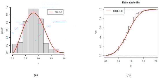
Figure 8. Plots of (a) the fitted PDF and (b) estimated CDF for the GOLE-E distribution for data set I.

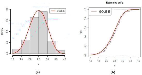
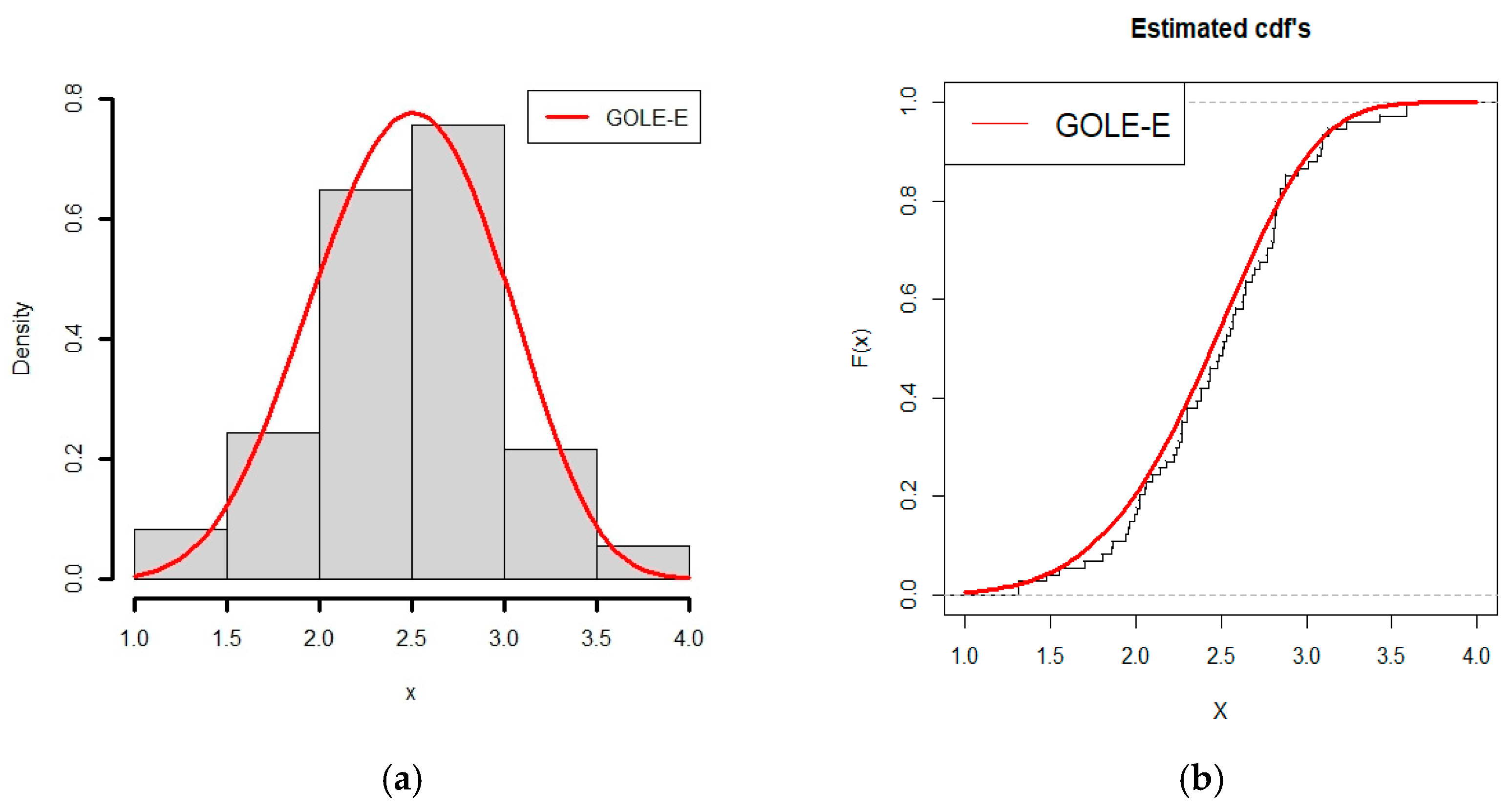
Figure 9. Plots of (a) the fitted PDF and (b) estimated CDF for the GOLE-E distribution for data set II.

6.2. Application of GOLE-W

The GOLE-W $\left(a,b,c,\lambda ,\beta \right)$ distribution with $\left(\lambda =1\right)$ is compared with some models, namely Weibull (W), moment exponential (ME), exponentiated Weibull (EW) (Mudholker and Srivastava, 1993 [23]), generalized Weibull (GW) (Lai 2014 [24]), beta Weibull (B-W) (Lee et al., 2007 [25]) and Kumaraswamy Weibull (Kw-W) (Cordeiro et al. 2010 [26]) distributions for all data sets.

Likewise, in Table 7, Table 8, Table 9 and Table 10, the MLEs, standard errors (in parentheses) and confidence interval [in brackets] of the parameters from all the competitive models along with AIC, CAIC, BIC and HQIC for the two data sets are presented. From these tables, it is quite obvious that for the two data sets, GOLE-W distribution is the best model with the lowest values of AIC, BIC, CAIC, HQIC, A*, W* and highest p-value of the K-S statistics. Hence, it is worth emphasizing that the proposed GOLE-F provides a more useful generalization (with exponential and Weibull as special models) than the competitive models for both of the datasets. A much more useful depiction is presented in the form of a visual comparison in Figure 10 and Figure 11, where the densities and distribution function of observed data are compared against the fitted models, respectively. These plots reveal that the proposed distributions provide the closest fit to all the observed data sets.

Table 7. MLEs, standard errors (in parentheses) and confidence interval [in brackets] values for data set I.

Models	$\widehat{\mathit{a}}$	$\widehat{\mathit{b}}$	$\widehat{\mathit{c}}$	$$\widehat{\mathit{\lambda }}$$	$$\widehat{\mathit{\beta }}$$
$$\begin{gathered} \mathrm{GOLE-W} \\ \left(a,b,c,\beta \right) \end{gathered}$$	2.3893	114.6653	4.8673	-	0.506777
	(2.1340)	(50.1098)	(2.1515)		(0.1582)
	[0, 6.57]	[16.45, 212.88]	[0.65, 9.08]		[0.20, 0.82]
$$\begin{gathered} \mathrm{Kw-W} \\ \left(a,b,\lambda ,\beta \right) \end{gathered}$$	0.7103	0.2623	-	3.0464	3.8368
	(0.0233)			(0.0263)	(0.0174)
	[0.66, 0.76]	[0.23,0.29]		[2.99, 3.10]	[3.80, 3.87]
$$\begin{gathered} \mathrm{B-W} \\ \left(a,b,\lambda ,\beta \right) \end{gathered}$$	0.7730	0.2276	-	3.0201	4.3742
	(0.0673)	(0.0137)		(0.0042)	(0.0042)
	[0.64, 0.90]	[0.20, 0.25]		[3.01, 3.02]	[4.37, 4.38]
$$\begin{gathered} \mathrm{E-W} \\ \left(b,\lambda ,\beta \right) \end{gathered}$$	-	0.8090	-	3.068922	0.9440
		(0.1515)		(0.3541)	(0.1732)
		(4.52, 6.53)		(2.475, 2.98)	[0.60, 1.28]
$$\begin{gathered} \mathrm{G-W} \\ \left(a,\lambda ,\beta \right) \end{gathered}$$	0.5597	-	-	2.7190	2.0240
	(11.2701)			(0.1140)	(0.7523)
	[0, 22.65]			[2.50, 2.94]	[0.55, 3.50]
$$\begin{gathered} \mathrm{M-E} \\ \left(b\right) \end{gathered}$$	-	0.406	-	-	-
		(0.016)
		[0.37, 0.44]
$$\begin{gathered} \mathrm{W} \\ \left(\lambda ,\beta \right) \end{gathered}$$	-	-	-	1.132926	2.71898
				(0.0623)	(0.1140)
				[1.01, 1.26]	[2.50, 2.94]

Table 8. The AIC, CAIC, BIC, HQIC, A*, W* and KS (p-value) values for data set I.

Models	AIC	CAIC	BIC	HQIC	A*	W*	KS (p-Value)
$$\begin{gathered} \mathrm{GOLE-W} \\ \left(a,b,c,\beta \right) \end{gathered}$$	230.11	230.23	245.49	236.23	2.51	0.44	0.10 (0.17)
$$\begin{gathered} \mathrm{Kw-W} \\ \left(a,b,\lambda ,\beta \right) \end{gathered}$$	231.86	231.96	247.23	237.97	2.57	0.45	0.11 (0.03)
$$\begin{gathered} \mathrm{B-W} \\ \left(a,b,\lambda ,\beta \right) \end{gathered}$$	232.84	232.95	248.22	238.96	2.67	0.46	0.12 (0.01)
$$\begin{gathered} \mathrm{E-W} \\ \left(b,\lambda ,\beta \right) \end{gathered}$$	232.42	232.39	243.86	236.91	2.81	0.48	0.12 (0.000)
$$\begin{gathered} \mathrm{G-W} \\ \left(a,\lambda ,\beta \right) \end{gathered}$$	233.56	233.63	245.09	238.15	2.97	0.51	0.24 (0.000)
$$\begin{gathered} \mathrm{M-E} \\ \left(b\right) \end{gathered}$$	388.70	392.55	388.71	390.24	6.49	1.09	0.23 (0.008)
$$\begin{gathered} \mathrm{W} \\ \left(\lambda ,\beta \right) \end{gathered}$$	231.56	231.88	239.25	234.62	2.97	0.51	0.14 (0.000)

Table 9. MLEs, standard errors (in parentheses), confidence interval values [in brackets] for data set II.

Models	$\widehat{\mathit{a}}$	$\widehat{\mathit{b}}$	$$\widehat{\mathit{c}}$$	$$\widehat{\mathit{\lambda }}$$	$$\widehat{\mathit{\beta }}$$
$$\begin{gathered} \mathrm{GOLE-W} \\ \left(a,b,c,\beta \right) \end{gathered}$$	6.9553	114.6653	20.1203	-	0.8448
	(6.6794)	(50.1098)	(6.6638)		(0.31433)
	[0,20.04]	[0, 27.65]	[7.06, 33.18]		[0.23, 1.46]
$$\begin{gathered} \mathrm{Kw-W} \\ \left(a,b,\lambda ,\beta \right) \end{gathered}$$	1.6646	1.0950	-	4.3675	0.0187
	(0.8438)	(0.5829)		(2.8871)	(0.0192)
	[0.01, 3.32]	[0.23, 0.29]		[0, 10.0262]	[0, 0.0564]
$$\begin{gathered} \mathrm{B-W} \\ \left(a,b,\lambda ,\beta \right) \end{gathered}$$	1.7401	0.9961	-	4.2987	0.0222
	(1.3064)	(0.9249)		(2.0778)	(0.0253)
	[0, 4.30]	[0, 2.81]		[0.23, 8.37]	[0, 0.07]
$$\begin{gathered} \mathrm{E-W} \\ \left(b,\lambda ,\beta \right) \end{gathered}$$	-	1.7298	-	4.3083	0.9440
		(0.7208)		(0.9066)	(0.1732)
		[0.32, 3.14]		[2.53, 6.09]	[0, 0.07]
$$\begin{gathered} \mathrm{G-W} \\ \left(a,\lambda ,\beta \right) \end{gathered}$$	1.5460	-	-	5.3816	0.0033
	(0.9021)			(0.4906)	(0.0008)
	[0, 3.3142]			[4.42, 6.34]	[0.002, 0.005]
$$\begin{gathered} \mathrm{M-E} \\ \left(b\right) \end{gathered}$$	-	0.406	-	-	-
		(0.016)
		[0.37, 0.44]
$$\begin{gathered} \mathrm{W} \\ \left(\lambda ,\beta \right) \end{gathered}$$	-	-	-	0.0036	5.7342
				(0.0009)	(0.2428)
				[0.0002, 0.0053]	[5.26, 6.21]

Table 10. The AIC, CAIC, BIC, HQIC, A*, W* and KS (p-value) values for data set II.

Models	AIC	CAIC	BIC	HQIC	A*	W*	KS (p-Value)
$$\begin{gathered} \mathrm{GOLE-W} \\ \left(a,b,c,\beta \right) \end{gathered}$$	110.57	111.15	119.79	114.25	0.25	0.031	0.06 (0.93)
$$\begin{gathered} \mathrm{Kw-W} \\ \left(a,b,\lambda ,\beta \right) \end{gathered}$$	111.06	112.83	120.08	114.98	2.27	0.037	0.08 (0.91)
$$\begin{gathered} \mathrm{B-W} \\ \left(a,b,\lambda ,\beta \right) \end{gathered}$$	111.32	112.90	120.13	115.99	0.26	0.038	0.07 (0.92)
$$\begin{gathered} \mathrm{E-W} \\ \left(b,\lambda ,\beta \right) \end{gathered}$$	118.33	118.72	122.89	120.68	0.31	0.075	0.098 (0.89)
$$\begin{gathered} \mathrm{G-W} \\ \left(a,\lambda ,\beta \right) \end{gathered}$$	113.84	113.13	123.02	119.15	0.30	0.052	0.08 (0.88)
$$\begin{gathered} \mathrm{M-E} \\ \left(b\right) \end{gathered}$$	388.70	392.55	388.71	390.24	6.49	1.09	0.23 (0.008)
$$\begin{gathered} \mathrm{W} \\ \left(\lambda ,\beta \right) \end{gathered}$$	117.45	116.61	121.77	117.91	0.29	0.037	0.09 (0.87)

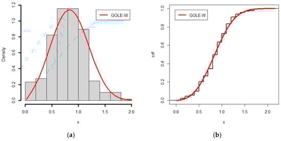
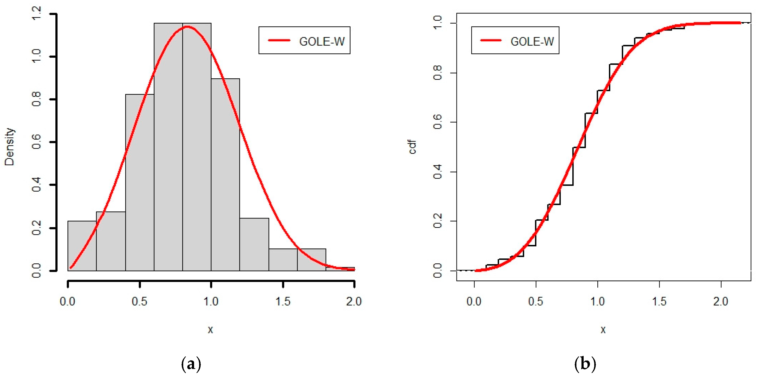
Figure 10. Plots of (a) the fitted PDF for the GOLE-W distribution and (b) estimated CDF for the GOLE-W distribution for data set I.

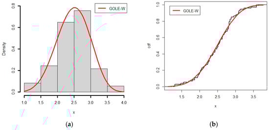
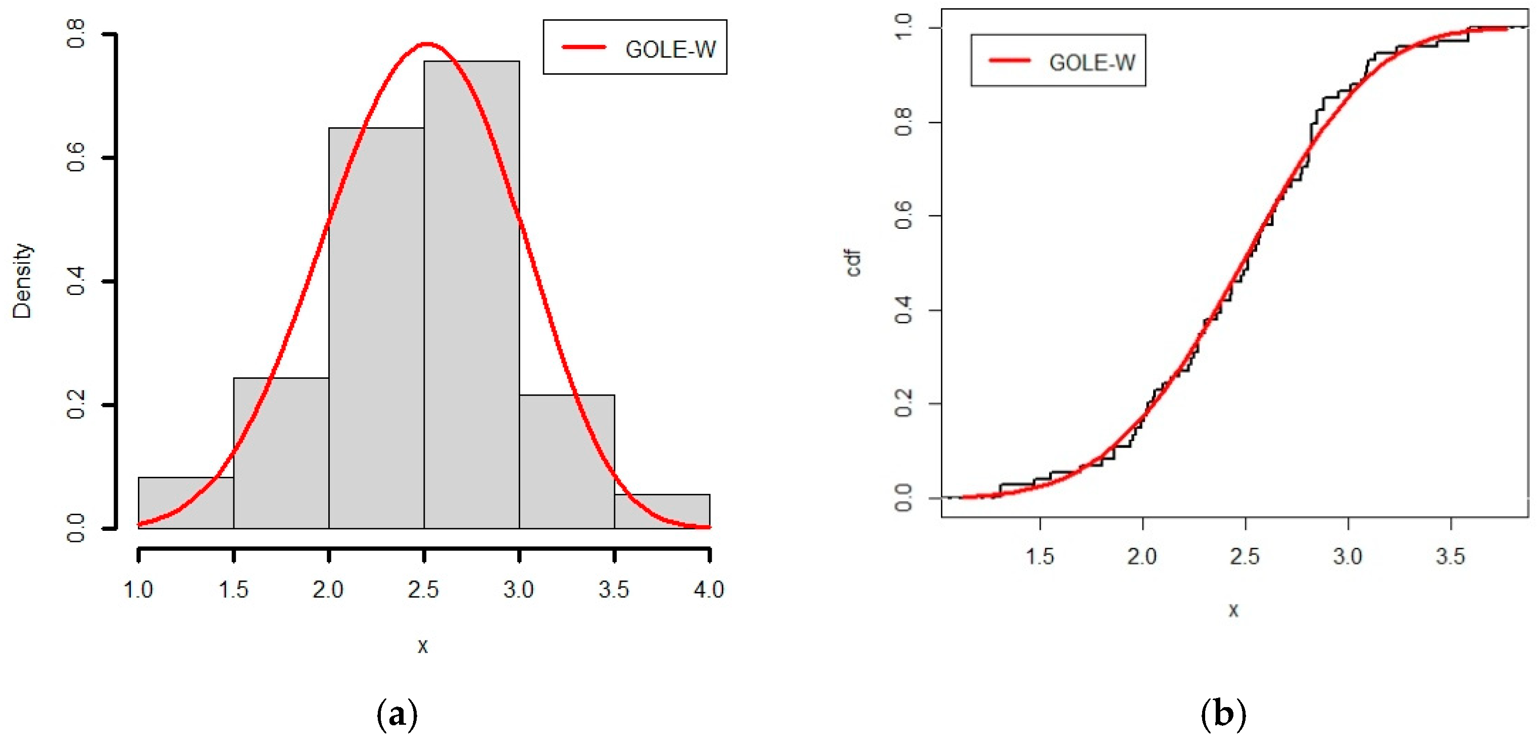
Figure 11. Plots of (a) the fitted PDF for the GOLE-W distribution and (b) estimated CDF for the GOLE-W distribution for data set II.

7. Conclusions

Through this paper, we provide a new general family of distributions to generalize any continuous baseline distribution. The main properties of the new family and other properties associated with the area of reliability are discussed. It was noted that the distributions generated by the new family are highly flexible in data modeling where we used one member to fit two real data to illustrate the importance of this family. This member provided consistently better fits than the other comparative distributions.

References

- Marshall, A.W. A new method for adding a parameter to a family of distributions with application to the exponential and Weibull families. Biometrika 1997, 84, 641–652. [Google Scholar] [CrossRef]
- Gupta, R.C.; Gupta, P.L.; Gupta, R.D. Modeling failure time data by Lehman alternatives. Commun. Stat.-Theory Methods 1998, 27, 887–904. [Google Scholar] [CrossRef]
- Eugene, N.; Lee, C.; Famoye, F. Beta-normal distribution and its applications. Commun. Stat. Theory Methods 2002, 31, 497–512. [Google Scholar] [CrossRef]
- Cordeiro, G.M.; De Castro, M. A new family of generalized distributions. J. Stat. Comput. Simul. 2011, 81, 883–898. [Google Scholar] [CrossRef]
- Alexander, C.; Cordeiro, G.M.; Ortega, E.M.; Sarabia, J.M. Generalized beta-generated distributions. Comput. Stat. Data Anal. 2012, 56, 1880–1897. Available online: https://EconPapers.repec.org/RePEc:eee:csdana:v:56:y:2012:i:6 (accessed on 19 May 2022). [CrossRef]
- Alzaatreh, A.; Lee, C.; Famoye, F. A new method for generating families of continuous distributions. Metron 2013, 71, 63–79. [Google Scholar] [CrossRef] [Green Version]
- Bourguignon, M.; Silva, R.B.; Cordeiro, G.M. The Weibull-G Family of Probability Distributions. J. Data Sci. 2014, 12, 53–68. Available online: http://www.jds-online.com/volume-12-number-1-january-2014 (accessed on 19 May 2022). [CrossRef]
- Tahir, M.H.; Cordeiro, G.M.; Alizadeh, M.; Mansoor, M.; Zubair, M.; Hamedani, G.G. The odd generalized exponential family of distributions with applications. J. Stat. Distrib. Appl. 2015, 2, 1. [Google Scholar] [CrossRef] [Green Version]
- Cordeiro, G.M.; Alizadeh, M.; Ortega, E.M.; Serrano, L.H.V. The Zografos-Balakrishnan odd log-logistic family of distributions: Properties and Applications. Hacet. J. Math. Stat. 2015, 46, 11781–11803. Available online: https://dergipark.org.tr/hujms/issue/43489/524407 (accessed on 19 May 2022). [CrossRef]
- Gomes-Silva, F.; Percontini, A.; De Brito, E.; Ramos, M.W.; Venâncio, R.; Cordeiro, G.M. The Odd Lindley-G Family of Distributions. Austrian J. Stat. 2017, 46, 65–87. [Google Scholar] [CrossRef] [Green Version]
- Alizadeh, M.; Cordeiro, G.M.; Pinho, L.G.B.; Ghosh, I. The Gompertz-G family of distributions. J. Stat. Theory Pract. 2016, 11, 179–207. [Google Scholar] [CrossRef]
- Jamal, F.; Nasir, M.A.; Tahir, M.H.; Montazeri, N.H. The odd Burr-III family of distributions. J. Stat. Appl. Probab. 2017, 6, 105–122. Available online: http://www.naturalspublishing.com/files/published/4nk6g57u5e512l.pdf (accessed on 19 May 2022). [CrossRef]
- Khan, S.; Balogun, O.S.; Tahir, M.H.; Almutiry, W.; Alahmadi, A.A. An Alternate Generalized Odd Generalized Exponential Family with Applications to Premium Data. Symmetry 2021, 13, 2064. [Google Scholar] [CrossRef]
- Sen, A.; Bhattacharyya, G.K. Inference procedures for the linear failure rate model. J. Stat. Plan. Inference 1995, 46, 59–76. [Google Scholar] [CrossRef]
- Shaked, M.; Shanthikumar, J.G. Stochastic Orders and Their Applications; Academic Press: San Diego, CA, USA, 2014. [Google Scholar] [CrossRef]
- Kotz, S.; Pensky, M. The Stress-Strength Model and Its Generalizations: Theory and Applications; World Scientific: Singapore, 2003. [Google Scholar] [CrossRef]
- Kundu, D.; Raqab, M.Z. Estimation of R = P (Y < X) for three-parameter Weibull distribution. Stat. Probab. Lett. 2009, 79, 1839–1846. [Google Scholar] [CrossRef]
- Aarset, M.V. How to Identify a Bathtub Hazard Rate. IEEE Trans. Reliab. 1987, 36, 106–108. [Google Scholar] [CrossRef]
- Dara, S.T.; Ahmad, M. Recent Advances in Moment Distribution and Their Hazard Rates; Lap Lambert Academic Publishing: Chisinau, Republic of Moldova, 2012. [Google Scholar]
- Hasnain, S.A.; Iqbal, Z.; Ahmad, M. On exponentiated moment exponential distribution. Pak. J. Stat. 2015, 31, 267–280. Available online: https://www.statindex.org/journals/1313/31/2 (accessed on 19 May 2022).
- Gupta, R.D.; Kundu, D. Exponentiated Exponential Family: An Alternative to Gamma and Weibull Distributions. Biom. J. 2001, 43, 117–130. [Google Scholar] [CrossRef]
- Nadarajah, S.; Kotz, S. The beta exponential distribution. Reliab. Eng. Syst. Saf. 2006, 91, 689–697. [Google Scholar] [CrossRef]
- Mudholkar, G.; Srivastava, D. Exponentiated Weibull family for analyzing bathtub failure-rate data. IEEE Trans. Reliab. 1993, 42, 299–302. [Google Scholar] [CrossRef]
- Lai, C.D. Generalized Weibull Distributions. In Generalized Weibull Distributions; Springer Briefs in Statistics; Springer: Berlin/Heidelber, Germany, 2014. [Google Scholar] [CrossRef]
- Lee, C.; Famoye, F.; Olumolade, O. Beta-Weibull Distribution: Some Properties and Applications to Censored Data. J. Mod. Appl. Stat. Methods 2007, 6, 173–186. [Google Scholar] [CrossRef]
- Cordeiro, G.M.; Ortega, E.M.; Nadarajah, S. The Kumaraswamy Weibull distribution with application to failure data. J. Frankl. Inst. 2010, 347, 1399–1429. [Google Scholar] [CrossRef]
Publisher’s Note: MDPI stays neutral with regard to jurisdictional claims in published maps and institutional affiliations. |
© 2022 by the authors. Licensee MDPI, Basel, Switzerland. This article is an open access article distributed under the terms and conditions of the Creative Commons Attribution (CC BY) license (https://creativecommons.org/licenses/by/4.0/).