Article

Accelerating Convergence for the Parameters of PV Cell Models

by
Lorentz Jäntschi
1 and
Mohamed Louzazni
2,*
1
Laboratory of Electrochemistry for Advanced Materials, Department of Physics and Chemistry, Technical University of Cluj-Napoca, 400114 Cluj-Napoca, Romania
2
Science Engineer Laboratory for Energy, National School of Applied Sciences, Chouaib Doukkali University of El Jadida, El Jadida P.O. Box 20, Morocco
*
Author to whom correspondence should be addressed.
Math. Comput. Appl. 2024, 29(1), 4; https://doi.org/10.3390/mca29010004
Submission received: 20 November 2023 / Revised: 8 January 2024 / Accepted: 9 January 2024 / Published: 10 January 2024

Abstract

:
Small-scale photovoltaic (PV) systems are essential for the local energy supply. The most commonly known PV cell is configured as a large-area p–n junction made from silicon, but PV systems today include PV cells of various manufactures and origins. The dependence relationship between current and voltage is nonlinear, known as the current–voltage characteristic. The values of the characteristic equation’s parameters define the working regime of the PV cell. In the present work, the parameter values are iteratively obtained by nonlinear regression for an explicit model. The acceleration of the convergence of these values is studied for an approximation simplifying the iterative calculation in the case of perpendicular offsets. The new estimations of parameters allow for a much faster estimate of the maximum power point of the PV system.

1. Introduction

Unlike heat, electricity is an organized form of energy; thus, the storage of energy in the form of electricity has a higher potential for exploitation compared to many other forms of storage, including in the form of chemical energy [1]. When it flows through a circuit, electricity produces heat and other forms of energy. This energy transfer is accompanied by an increase in entropy, as the electrical energy is transformed into other forms of energy, which are less organized and more disordered [2]. At the same time, the transportation of electrical energy has seen major advances [3], with global power grids emerging as the dominant form of energy supply today.
The ensemble of global power networks is a complex one, but it benefits from a number of major advantages, such as the working regime of consumers (industrial and domestic) being regularized by the diurnal cycle [4]. The diurnal cycle is also regulated by its smallest entity, part of an electricity production network, i.e., photovoltaics (PV), which are referred to in this work, by virtue of their light source [5].
One of the advantages of the large-scale proliferation of PV from high-power producers to consumers—which, through the use of photovoltaic panel systems—are also small producers, is that it brings the source closer to the consumer, thus eliminating at least some of the transport losses [6,7,8]. The ideal is, of course, for each of these consumers to be able to cover their energy needs from their own sources, and photovoltaic cell systems represent the most appropriate solution, since, in addition to the other arguments, they offer very good coverage of the working regime of the consumers in the immediate vicinity, i.e., during the day. However, this is not (yet) possible for all instances; thus, the integration of small-scale electricity production systems into global electricity networks is a priority [9,10,11].
One of the problems to be addressed regarding the integration of PV cells in complex systems and networks is the estimation of their working regime—in other words, their current vs. voltage response, also known as their characteristic equation [12,13,14].
From the start, it should be stated that there are many types of PV units [15,16,17], and there is not one model that is considered a universal solution. Even if there were only one type of PV unit, the model would probably still not be universal. There are (small) intrinsic variations in their operating parameters due to the technological process, quality (purity), and specificity (microcomposition) of the materials used [18,19,20,21].
An analytical solution for the current flow through a diode [22] and PV [23] may serve to derive accurate expressions for solar cell fill factors [24]. Even so, there are a number of models that approximate the behavior of PV cells based on the behavior of an idealized system consisting of a series of active and passive components (see the Single Diode, Double Diode and PV Generators Models section in [25] and references therein). Unfortunately, this model is not at all simple; it has an analytical expression, but the function that expresses the value of voltage as a function of current is accessible only by numerical means, only providing the value of the available current and requiring a series of repeated numerical evaluations (the same can be said of the function that expresses the value of current as a function of voltage). The classic approach involves the use of the Lambert function, providing voltage as a function of current (or vice versa), which is a mathematical formalization of the fact that the function expressing voltage as a function of current (or vice versa) requires a series of successive approximations, which are formalized by the same general framework defined by the equation and the associated function proposed by Lambert, i.e., z = W ( z ) exp ( W ( z ) ) (for further details, see the Lambert Function section in [25,26]). An alternate approach is to use explicit equations approximating the voltage vs. current (or vice versa) dependence (see the Explicit equations section in [25]). Either way, the associated problem in this context is the correct and fast identification of model parameters—parameters that are usually constructional (depending on the construction of the PV cell) and which may also depend on the working regime (temperature and solar radiation spectrum).
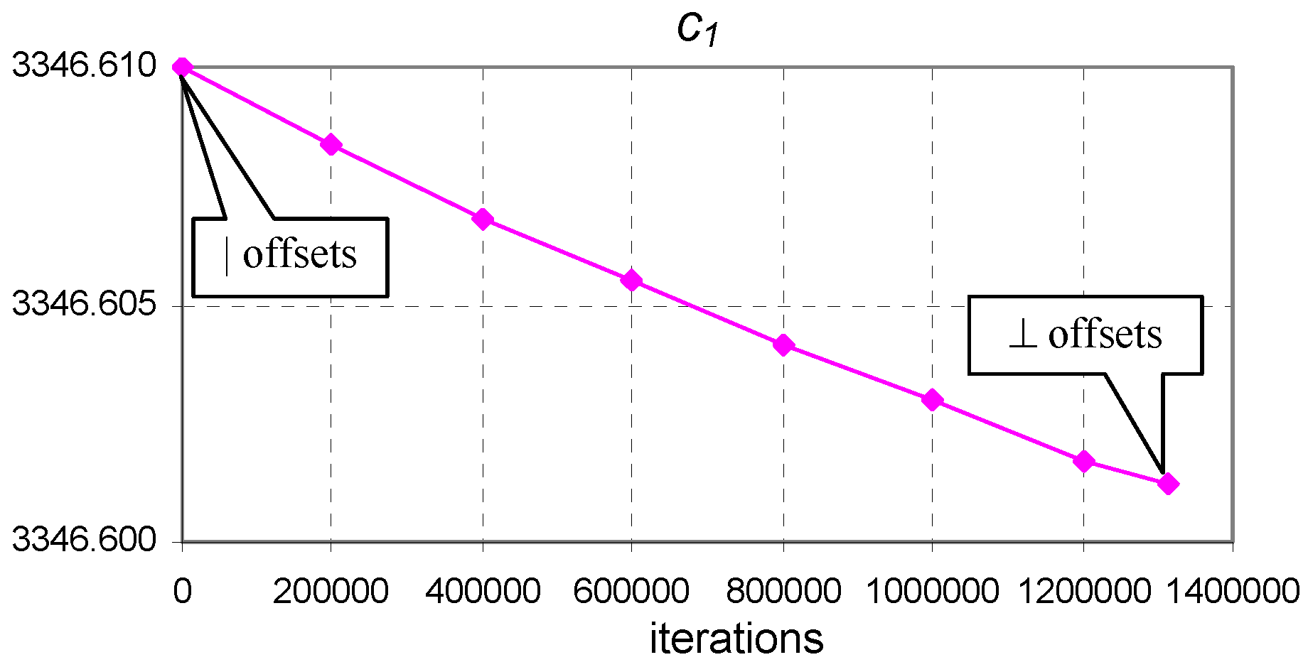
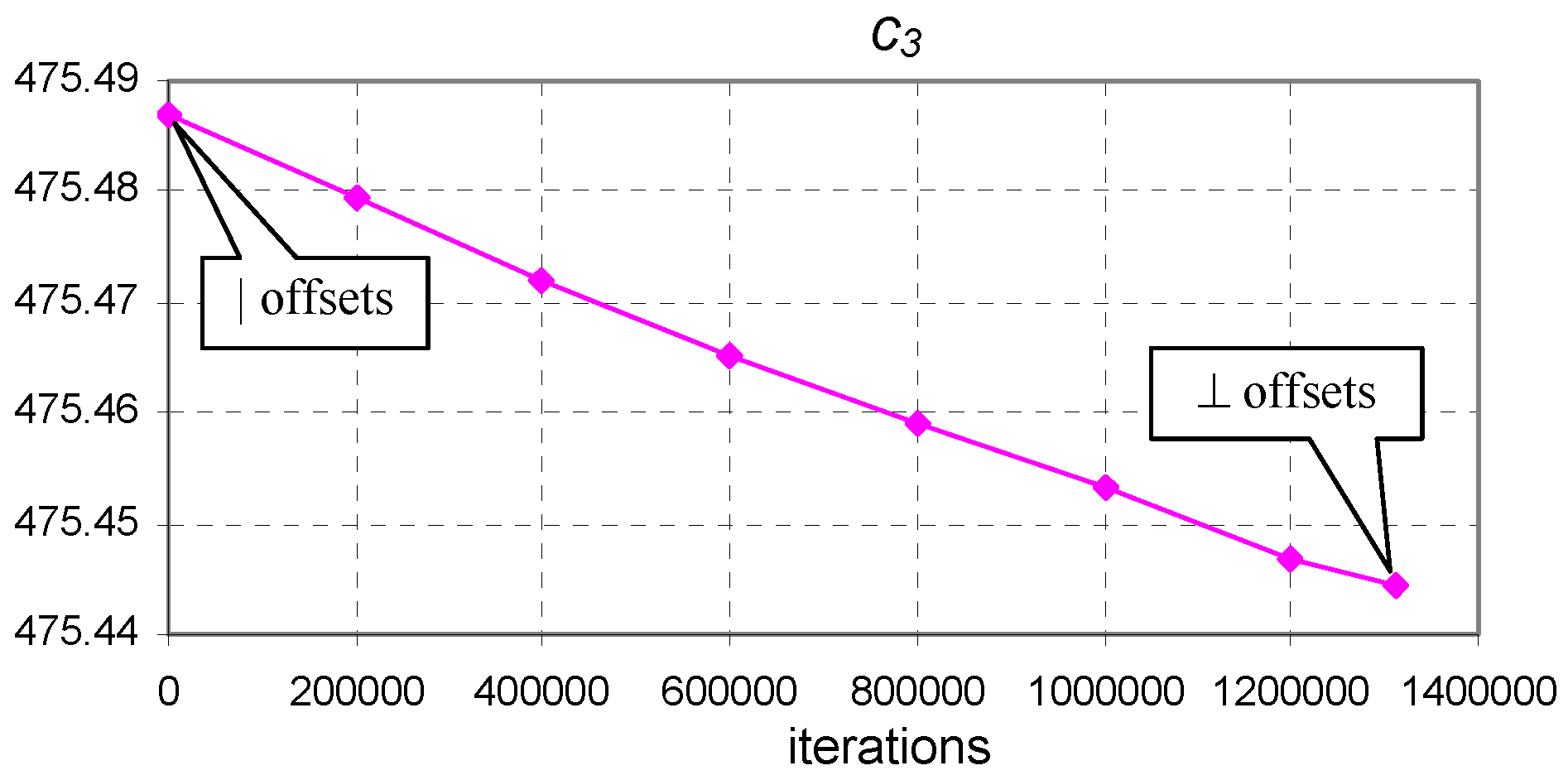
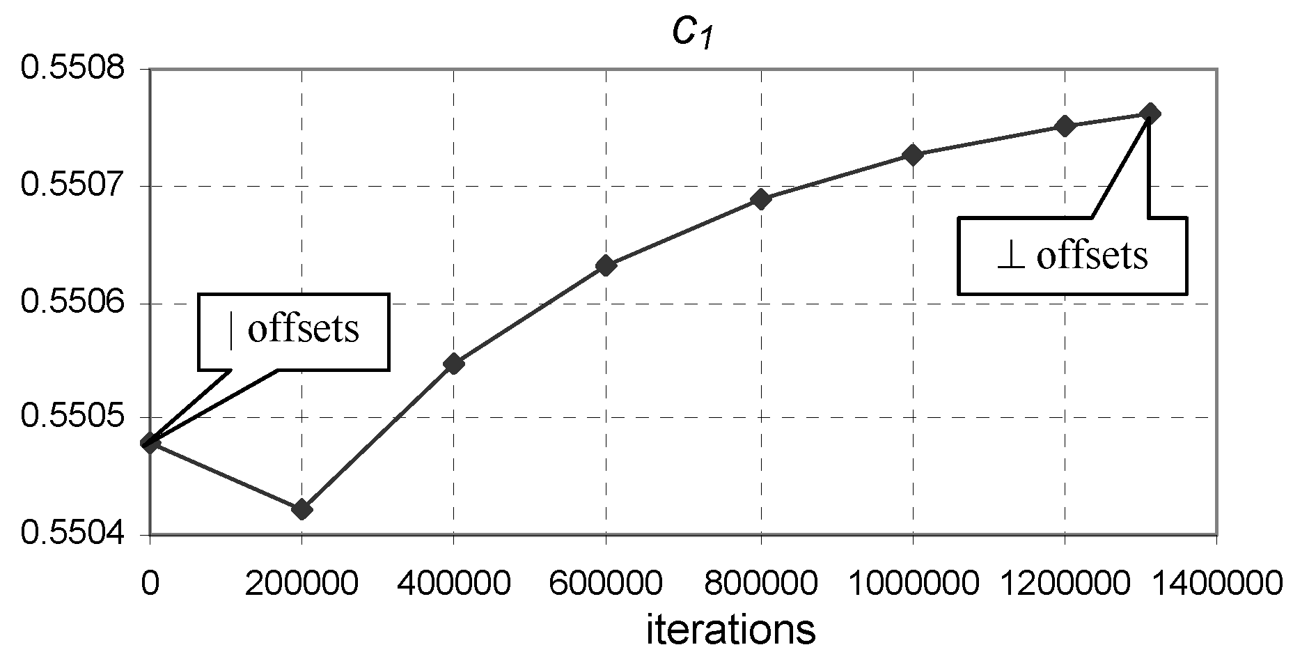
The classic method adopted by the implementations in use is to identify the regression parameters using a construction that fixes the experimental error on only one of the variables, namely that for which the value of the nonlinear function is expressed and which is positioned on the vertical axis in the representation (vertical offsets). The alternative route considers the offsets to be perpendicular, assuming that both paired observations are affected by the error [25,27,28].
With respect to the classical approaches, particle swarm optimization is a very well-established and powerful population-based metaheuristic for parameter estimation of PV cells and modules; a series of studies have addressed this issue in depth [29,30,31,32,33,34].
In [25], the full approach of perpendicular offsets was employed to identify the parameters for two nonlinear regressions. The perpendicular offsets approach achieves correct physical meaning by minimizing experimental errors of both a voltmeter and ammeter against the classical vertical offsets approach, which minimizes only one series of errors, the others being considered to correspond to true values. However, the use of perpendicular offsets instead of vertical offsets creates another issue: the problem of parameter identification is not a simple problem of nonlinear optimization anymore but an embedded nonlinear optimization inside another nonlinear optimization (see Algorithms 1 to 3 in [25]). In this case, a simplified approach is proposed, which accelerates the convergence to the optimum values of the parameters. For the sake of comparison, the same data and the same models are used. Two additional datasets reported in the literature were also subjected to the same analysis here.

2. Materials and Methods

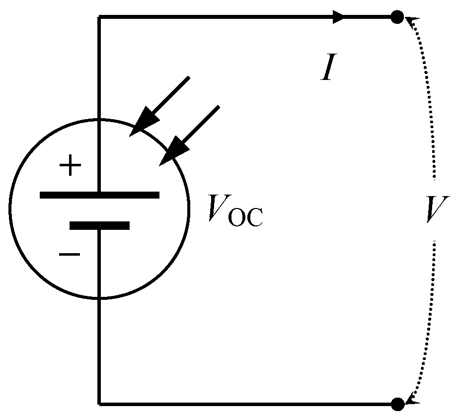
A data series used in this study are presented in Table 1 of [25] representing a series of current vs. voltage paired measurements taken for a PV cell (Figure 1).
In a plot of current (I) as a univariate function (generically written as y = f ( x ; c ) , explicitly expressing some general parameter’s (c) current as a function of voltage) of voltage (V), vertical offsets have units of amperes (A, or multiples/submultiples thereof, as the case may be), while horizontal offsets have units of volts (V, or multiples/submultiples thereof, as the case may be). One is translated into another by resistance ( Ω ) and/or conductance ( Ω 1 ). Using the same units (either A or V), oblique offsets also have meaning.
The tangent is expressed as Equation (1).
y = f ( z i ; c ) + ( x z i ) f ( z i ; c ) ,
Equation (1) is the equation of the tangent to y = f ( x ; c ) in x = z i ( z i is the ordinate position of the contact point between the tangent and the curve), and f ( x ; c ) is the function derivative ( f ( x ; c ) = d f ( x ; c ) / d x ) (see Figure 2).
The directions normal to the y = f ( x ) curve (Figure 2) is expressed as Equation (2).
y = f ( z i ; c ) ( x z i ) / f ( z i ; c )
The contact point is ( z i , f ( z i ; c ) ) , and the normal direction intersects the observation point ( x i , y i ) , so (using Equation (2)):
y i = f ( z i ; c ) ( x i z i ) / f ( z i ; c )
The numeric value of z i can be obtained from Equation (3) by root finding. With the value of z i , the value of the perpendicular offset d i is given in Equation (4).
d i 2 = ( z i x i ) 2 + ( f ( z i ; c ) y i ) 2
Alternately to the root finding in Equation (3), in most cases (for smooth variations), it is enough to find the z i for which d i is minimum; this is the exact approach involving the use of perpendicular offsets used in [25].
For each observed pair ( ( x i , y i ) from a set of n), the vertical offset is | y i f ( x i ; c ) | , while the horizontal offset is | x i f 1 ( y i ; c ) | , such that the height ( h i ) of a triangle with these two offsets as legs is expressed by Equation (5).
h i 2 = ( f ( x i ; c ) y i ) 2 ( f 1 ( y i ; c ) x i ) 2 ( f ( x i ; c ) y i ) 2 + ( f 1 ( y i ; c ) x i ) 2
This height ( h i , Equation (5)) approximates ( h i d i , Figure 3) the length of the perpendicular offset ( d i , Equation (4).
In the proposed approach, I ( V ) (or V ( I ) ) is expressed as a nonlinear function of the parameters (c). Afterwards, these c values ( c 1 , c 2 , , c n ) can be determined by optimizing an objective function such as the sum of heights squares.
It should be noted that when the inverse of the function ( f 1 in Equation (5)) is available and explicit, the use of Equation (5) does not require root finding (solving of Equation (3)) or minimization (of Equation (4)). This is the main advantage of the proposed method, and the hope is that it will dramatically reduce the number of iterations until optimum values (accelerated convergence).
Let us set
g ( c ) = h i 2 ,
with h i 2 from Equation (5).
If Minimize( g , c ) solves an optimization problem where g is the objective function to be minimized and c represents the unknown coefficients (to be found) on which the value of the objective function depends, then the iteration to the optimal values is as follows:
  • c optimum values from minimizing the sums of the residuals with classical vertical offsets ( i = 1 m ( y i f ( x i ; c ) ) 2 );
  • Minimize( g , c ).
Optimization works by finding the adjustable parameters (c) for which g ( c ) is minimum.
When compared with the previous approach (Algorithms 1 to 3 in [25]), in this case, the optimization problem is considerably simplified; an inner-loop optimization is no longer required. For the sake of comparison, the same software environment as that reported in [25] was used for implementation.
Two cases were investigated as in [25] here also (Equation (7)):
f ( x ; c ) = f 1 ( x ; c ) , if U = U ( I ) f 2 ( x ; c ) , if I = I ( U )
with:
f 1 ( x ; c ) = c 1 + c 2 x c 3 x 2 c 4 + x
and
f 2 ( x ; c ) = c 1 exp ( c 2 + c 3 ln ( x ) )
In Equations (8) and (9), the signs preceding the coefficients were conveniently chosen. The number of parameters (m) is 4 for f 1 and 3 for f 2 (see Equations (8) and (9)).
The coefficients of f 1 are derived by assigning U to the vertical axis ( y U ) and I to the horizontal axis ( x I ), while the coefficients of f 2 are derived by assigning I to the vertical axis ( y I ) and U to the horizontal axis ( x U ).

3. Case Studies

Experimental data provided in [25] were used. For convenience, the dataset was designated as Pink, and the ( U ( mV ) , I ( mA ) ) paired measurements were as follows:
  • Pink (n = 17): (1132, 1.147), (1110, 1.187), (1080, 1.257), (1038, 1.312), (1010, 1.362), (973, 1.406), (930, 1.480), (900, 1.493), (845, 1.556), (772, 1.609), (703, 1.672), (593, 1.742), (493, 1.776), (405, 1.785), (332, 1.812), (254, 1.821), and (163, 1.834).
As in [25], the models ( f 1 for V = V ( I ) and f 2 for I = I ( V ) ) were applied to the Pink PV cell data.
Experimental data were extracted from [35] regarding current–voltage characteristics (Figure 5 in [35]) of two PV cells (designated as Blue and Gray). The ( U ( V ) , I ( A ) ) paired measurements were as follows:
  • Blue (n = 8): (0.1019, 0.1011), (0.1997, 0.1015), (0.3006, 0.1007), (0.3994, 0.0974), (0.4680, 0.0830), (0.4992, 0.0597), (0.5169, 0.0395), and (0.5294, 0.0189);
  • Gray (n = 13): (0.1007, 0.5565), (0.1503, 0.5546), (0.2008, 0.5498), (0.2503, 0.5413), (0.3009, 0.5318), (0.3266, 0.5242), (0.3504, 0.5137), (0.3742, 0.4985), (0.3990, 0.4671), (0.4219, 0.4253), (0.4505, 0.3482), (0.4743, 0.2579), (0.4981, and 0.1504).
Model f 2 for I = I ( V ) was applied to the Blue and Gray PV cell data.

4. Results and Discussion

4.1. Pink Dataset

With the modified forms of the nonlinear Equations (8) and (9), all coefficients are positive. The classical vertical offsets approach using any modeling software may produce the initial estimates of the coefficients. FindGraph [36] was used here. Table 1 contains these estimates.
Very good agreement between the data and the model was obtained from the beginning (see Statistics in Table 1). Less than 1% of the total variation was not been explained by either model ( 1 r adj 2 is 2.3‰ for f 1 and 1.3‰ for f 2 ). The model provided by f 2 has a much higher statistical significance than the model provided by f 1 (a simple comparison of F values suffices as proof); the model provided by f 1 is also more robust (it has only three degrees of freedom, i.e., its parameters).
The value of R S S is a special quantity and is available only from perpendicular offsets representing their squared sum. As the values show (see R S S in Table 1), the R S S quantity is independent of the selection of the axis in the plot. It is worth remembering (see Equation (7)) that the coefficients of f 1 were derived by assigning U to the vertical axis ( y U ) and I to the horizontal axis ( x I ), while the coefficients of f 2 were derived by assigning I to the vertical axis ( y I ) and U to the horizontal axis ( x U ). Independent of the assignment, the perpendicular offsets have the same meanings, and their values enable comparison between the models. Again, f 2 is a better choice for modeling the I vs. U characteristic (the unexplained variance ( R S S ) is smaller; see Table 1).
With a powerful nonlinear optimization library, such as (from personal experience) Mathcad [37], Mathematica [38], or Matlab [39], or even open libraries (AlgLib in [25]), only the statement of the problem in the formalism of the library must be given. As reported in the Materials and Methods section, the algorithm is simple. It involves estimating the initial values of the parameters (C) from the classical Gaussian vertical offsets of the selected model (Equation (8) or (9)) of nonlinear regression, followed by running of minimization for Σ i = 1 n h i 2 . The convergence is fast. The optimum values of the parameters for f 1 are obtained according the values presented in Table 1 after 1,307,759 iterations, which is, compared with the exact method of perpendicular offsets (see §3.2. The Numerical Results in [25]), a significant gain in speed. The convergence is accelerated even faster in the case of f 2 ; only 958 iterations were necessary, making it roughly 1,000,000 times faster.
Table 2 presents the optimized values of the parameters.
The final values of the coefficients of f 1 are nearly identical to the initial values provided by the vertical offsets. The evolution of the parameters is depicted, for convenience, in Figure 4, Figure 5, Figure 6 and Figure 7.
Figure 4, Figure 5, Figure 6 and Figure 7 show that coefficients c 1 to c 4 exhibited small changes. The reason for this behavior is that the perpendicular offsets being nearly as long as the vertical ones and the length of the horizontal offset being much longer in comparison. Considering the meaning of a horizontal (voltage measurement errors), vertical (current measurement errors), and perpendicular (combined measurement errors) offset, we can assume that experimental error produced as a result of the use of a voltmeter was much smaller than the experimental error produced by the use of an ammeter. For convenience, the values of the horizontal and vertical offsets for the optimum values of the coefficients are easily extracted from the values presented in Table 3.
The final values of the coefficients of f 2 are nearly identical to the initial values provided by vertical offsets. The evolution of the parameters is depicted, for convenience, in Figure 8, Figure 9 and Figure 10.
Figure 8, Figure 9 and Figure 10 show that only the c 1 coefficient exhibited visible changes. The reason for this behavior is that the perpendicular offsets are nearly as long as the vertical ones, the length of the horizontal offset being much longer in comparison. For convenience, the values of the horizontal and vertical offsets for the optimum values of the coefficients are easily extracted from the values presented in Table 4.
Open-circuit voltage ( V oc , which is V = V ( I ) for I 0 ), short-circuit intensity ( I sc , which is I = I ( V ) for V 0 ), internal resistance ( r i ), maximum power point ( P mpp , which is max ( V · I ) ), the current intensity ( I mpp ), and the electric potential (voltage) ( V xp ) at maximum power are key parameters for accurate estimation of the working regime of a PV cell and are directly calculable from the final parameter values of the model.
For the case considered here, the changes in the values of the PV parameters are small (Table 5).
The model of I = I ( V ) with f 2 provided the highest association between observed and calculated values (F = 9543 in Table 2) and the fastest convergence when changed from vertical to perpendicular offsets.

4.2. Blue and Gray Datasets

Results are given in Table 6.
The convergence from vertical offsets to perpendicular offsets achieved using the proposed approach (Equation (5)) was fast. It required 23,470 evaluations of i = 1 8 h i 2 for the Blue cell (Figure 11, Figure 12 and Figure 13) and 1,313,355 evaluations of i = 1 13 h i 2 for the Gray cell (Figure 14, Figure 15 and Figure 16).
As Figure 4, Figure 5, Figure 6, Figure 7, Figure 8, Figure 9, Figure 10, Figure 11, Figure 12, Figure 13, Figure 14, Figure 15 and Figure 16 reveal, similar behavior is reflected by all obtained results, and the changes in the parameters of the PV cells due to shifting from vertical to perpendicular offsets are small. Considering the amount of calculation required, the gain may even be seen as insignificant. The gain in approximating the perpendicular offsets with the offset triangle heights (Equation (5)) is considerable—in one case, the convergence was 2000 faster, while in another, it was 2,000,000 times faster. This speedup is mainly due to the elimination of the inner non-linear optimization loop reported in [25].
Using h i 2 (Equation (5)) instead of d i 2 (Equation (4)) is yet another approximation in finding the optimal values of the parameters (c) that provide the best fit of the selected model ( f ( x ; c ) ) to the experimental data ( ( x i , y i ) , i = 1 , 2 , , n ). However, the g ( c ) objective function is the sum of residuals with the same direction as the perpendicular offsets, and its maximum is the sum of the squared perpendicular offsets. If the values proposed by the approximated perpendicular offsets still do not fully meet accuracy requirements, then the initial values for the exact approach of perpendicular offsets can definitely be used as a new guess, thus accelerating the convergence of the model and PV cell parameters.
There is no uncertainty in the output—only in the input. Both the Levenberg–Marquardt algorithm (used for backend nonlinear optimization) and the proposed implementation are fully deterministic. Each independent run on the same data and the same model leads to exactly the same results. However, using stochastic assignments in the software implementation may improve the convergence in certain cases, although likely not significantly, on average.

5. Conclusions and Forthcoming Work

The perpendicular offsets approach is suited for sets of paired data. Nonlinear regression with perpendicular offsets may take a considerable amount of iterations to obtain optimal values of the parameters. Convergence is significantly accelerated when approximate perpendicular offsets are calculated instead of exact offsets. The proposed calculation approach may be suited for embedding into physical devices for industrial applications. Other calculation alternatives are still open to be explored, including calculation based on maximization of likelihood. However, in the case considered here, mathematical optimization performed very well.

Author Contributions

Conceptualization, L.J.; methodology, L.J.; software, L.J.; validation, L.J.; formal analysis, L.J. and M.L.; investigation, L.J. and M.L.; resources, L.J. and M.L.; data curation, L.J. and M.L.; writing—original draft preparation, L.J.; writing—review and editing, L.J. and M.L.; visualization, L.J. and M.L.; supervision, L.J.; project administration, M.L.; funding acquisition, M.L. All authors have read and agreed to the published version of the manuscript.

Funding

This research received no external funding.

Data Availability Statement

No new data were created. The experimental and numerical data used to support the findings of this study are included within the article.

Acknowledgments

Help in improving this manuscript from anonymous reviewers was greatly appreciated.

Conflicts of Interest

The authors declare that they have no conflicts of interest.

Abbreviations

The following abbreviations are used in this manuscript:
PVPhotovoltaic
RSSResidual sum of squares
FFisher’s F value
r adj 2 Ajusted determination coefficient
MSEMean square error

References

  1. Armaroli, N.; Balzani, V. The Future of Energy Supply: Challenges and Opportunities. Angew. Chem. Int. Ed. 2007, 46, 52–66. [Google Scholar] [CrossRef]
  2. Feistel, R.; Ebeling, W. Entropy and the Self-Organization of Information and Value. Entropy 2016, 18, 193. [Google Scholar] [CrossRef]
  3. Hao, J.; Yang, Y.; Xu, C.; Du, X. A comprehensive review of planning, modeling, optimization, and control of distributed energy systems. Carb. Neutrality 2022, 1, 28. [Google Scholar] [CrossRef]
  4. Karalus, S.; Köpfer, B.; Guthke, P.; Killinger, S.; Lorenz, E. Analysing Grid-Level Effects of Photovoltaic Self-Consumption Using a Stochastic Bottom-up Model of Prosumer Systems. Energies 2023, 16, 3059. [Google Scholar] [CrossRef]
  5. Balan, M.; Damian, M.; Jäntschi, L. Preliminary Results on Design and Implementation of a Solar Radiation Monitoring System. Sensors 2008, 8, 963–978. [Google Scholar] [CrossRef]
  6. Devabhaktuni, V.; Alam, M.; Shekara Sreenadh Reddy Depuru, S.; Green, R.C.; Nims, D.; Near, C. Solar energy: Trends and enabling technologies. Renew. Sustain. Energy Rev. 2013, 19, 555–564. [Google Scholar] [CrossRef]
  7. Kumar, P.N.; Selvakumar, B.; R, V.; Rajkumar, K.; Kumar, K.K.; Kamaraja, A.S. Smart Grid Peer-to-Peer Exchanging Energy System using Block Chain. In Proceedings of the 2023 7th International Conference on Computing Methodologies and Communication (ICCMC), Erode, India, 23–25 February 2023; pp. 1036–1040. [Google Scholar] [CrossRef]
  8. Boyko, E.; Byk, F.; Ilyushin, P.; Myshkina, L.; Suslov, K. Methods to improve reliability and operational flexibility by integrating hybrid community mini-grids into power systems. Energy Rep. 2023, 9, 481–494. [Google Scholar] [CrossRef]
  9. Mohd, A.; Ortjohann, E.; Schmelter, A.; Hamsic, N.; Morton, D. Challenges in integrating distributed energy storage systems into future smart grid. In Proceedings of the 2008 IEEE International Symposium on Industrial Electronics, Cambridge, UK, 30 June–2 July 2008; pp. 1627–1632. [Google Scholar] [CrossRef]
  10. Mahmud, K.; Khan, B.; Ravishankar, J.; Ahmadi, A.; Siano, P. An internet of energy framework with distributed energy resources, prosumers and small-scale virtual power plants: An overview. Renew. Sustain. Energy Rev. 2020, 127, 109840. [Google Scholar] [CrossRef]
  11. Wu, Y.; Wu, Y.; Guerrero, J.M.; Vasquez, J.C. A comprehensive overview of framework for developing sustainable energy internet: From things-based energy network to services-based management system. Renew. Sustain. Energy Rev. 2021, 150, 111409. [Google Scholar] [CrossRef]
  12. Mehta, H.K.; Warke, H.; Kukadiya, K.; Panchal, A.K. Accurate Expressions for Single-Diode-Model Solar Cell Parameterization. IEEE J. Photovolt. 2019, 9, 803–810. [Google Scholar] [CrossRef]
  13. Farooq, W.A.; Elgazzar, E.; Dere, A.; Dayan, O.; Serbetci, Z.; Karabulut, A.; Atif, M.; Hanif, A. Photoelectrical characteristics of novel Ru(II) complexes based photodiode. J. Mater. Sci. Mater. Electron. 2019, 30, 5516–5525. [Google Scholar] [CrossRef]
  14. Yükseltürk, E.; Surucu, O.; Terlemezoglu, M.; Parlak, M.; Altındal, Ş. Illumination and voltage effects on the forward and reverse bias current–voltage (I-V) characteristics in In/In2S3/p-Si photodiodes. J. Mater. Sci. Mater. Electron. 2021, 32, 21825–21836. [Google Scholar] [CrossRef]
  15. Khatibi, A.; Razi Astaraei, F.; Ahmadi, M.H. Generation and combination of the solar cells: A current model review. Energy Sci. Eng. 2019, 7, 305–322. [Google Scholar] [CrossRef]
  16. Benda, V.; Černá, L. PV cells and modules—State of the art, limits and trends. Heliyon 2020, 6, e05666. [Google Scholar] [CrossRef]
  17. Yang, B.; Wang, J.; Zhang, X.; Yu, T.; Yao, W.; Shu, H.; Zeng, F.; Sun, L. Comprehensive overview of meta-heuristic algorithm applications on PV cell parameter identification. Energy Convers. Manag. 2020, 208, 112595. [Google Scholar] [CrossRef]
  18. Brabec, C.J.; Distler, A.; Du, X.; Egelhaaf, H.J.; Hauch, J.; Heumueller, T.; Li, N. Material Strategies to Accelerate OPV Technology Toward a GW Technology. Adv. Energy Mater. 2020, 10, 2001864. [Google Scholar] [CrossRef]
  19. Shi, M.; Wang, T.; Wu, Y.; Sun, R.; Wang, W.; Guo, J.; Wu, Q.; Yang, W.; Min, J. The Intrinsic Role of Molecular Mass and Polydispersity Index in High-Performance Non-Fullerene Polymer Solar Cells. Adv. Energy Mater. 2021, 11, 2002709. [Google Scholar] [CrossRef]
  20. Yang, W.; Wang, W.; Wang, Y.; Sun, R.; Guo, J.; Li, H.; Shi, M.; Guo, J.; Wu, Y.; Wang, T.; et al. Balancing the efficiency, stability, and cost potential for organic solar cells via a new figure of merit. Joule 2021, 5, 1209–1230. [Google Scholar] [CrossRef]
  21. Meddeb, H.; Götz-Köhler, M.; Neugebohrn, N.; Banik, U.; Osterthun, N.; Sergeev, O.; Berends, D.; Lattyak, C.; Gehrke, K.; Vehse, M. Tunable Photovoltaics: Adapting Solar Cell Technologies to Versatile Applications. Adv. Energy Mater. 2022, 12, 2200713. [Google Scholar] [CrossRef]
  22. Banwell, T.; Jayakumar, A. Exact analytical solution for current flow through diode with series resistance. Electron. Lett. 2000, 36, 291–292. [Google Scholar] [CrossRef]
  23. Jain, A.; Kapoor, A. Exact analytical solutions of the parameters of real solar cells using Lambert W-function. Sol. Energy Mater. Sol. Cells 2004, 81, 269–277. [Google Scholar] [CrossRef]
  24. Green, M.A. Accurate expressions for solar cell fill factors including series and shunt resistances. Appl. Phys. Lett. 2016, 108, 081111. [Google Scholar] [CrossRef]
  25. Jäntschi, L. Symmetry in Regression Analysis: Perpendicular Offsets–The Case of a Photovoltaic Cell. Symmetry 2023, 15, 948. [Google Scholar] [CrossRef]
  26. Garcia, A.S.; Strandberg, R. Analytical Modeling of the Maximum Power Point with Series Resistance. Appl. Sci. 2021, 11, 10952. [Google Scholar] [CrossRef]
  27. Jäntschi, L. Potential of Electrical Cells: The Effect of the Experimental Design on the Results. In Proceedings of the 2023 8th International Conference on Clean Electrical Power—Renewable Energy Resources Impact (ICCEP), Terrasini, Italy, 27–29 June 2023; pp. 622–629. [Google Scholar] [CrossRef]
  28. Stoenoiu, C.E.; Jäntschi, L. Simultaneous Determinations for the Internal Resistance of Three Batteries. Three Analytical Methods Involved. In Proceedings of the 2023 10th International Conference on Modern Power Systems (MPS), Cluj-Napoca, Romania, 21–23 June 2023; p. P146. [Google Scholar] [CrossRef]
  29. Jordehi, A.R. Time varying acceleration coefficients particle swarm optimisation (TVACPSO): A new optimisation algorithm for estimating parameters of PV cells and modules. Energy Convers. Manag. 2016, 129, 262–274. [Google Scholar] [CrossRef]
  30. Rezaee Jordehi, A. Enhanced leader particle swarm optimisation (ELPSO): An efficient algorithm for parameter estimation of photovoltaic (PV) cells and modules. Sol. Energy 2018, 159, 78–87. [Google Scholar] [CrossRef]
  31. Jordehi, A.R. Binary particle swarm optimisation with quadratic transfer function: A new binary optimisation algorithm for optimal scheduling of appliances in smart homes. Appl. Soft Comput. 2019, 78, 465–480. [Google Scholar] [CrossRef]
  32. Rezaee Jordehi, A. A mixed binary-continuous particle swarm optimisation algorithm for unit commitment in microgrids considering uncertainties and emissions. Int. Trans. Electr. Energy Syst. 2020, 30, e12581. [Google Scholar] [CrossRef]
  33. Rezaee Jordehi, A. Particle swarm optimisation with opposition learning-based strategy: An efficient optimisation algorithm for day-ahead scheduling and reconfiguration in active distribution systems. Soft Comput. 2020, 24, 18573–18590. [Google Scholar] [CrossRef]
  34. Rezaee Jordehi, A. An improved particle swarm optimisation for unit commitment in microgrids with battery energy storage systems considering battery degradation and uncertainties. Int. J. Energy Res. 2021, 45, 727–744. [Google Scholar] [CrossRef]
  35. Charles, J.; Abdelkrim, M.; Muoy, Y.; Mialhe, P. A practical method of analysis of the current-voltage characteristics of solar cells. Sol. Cells 1981, 4, 169–178. [Google Scholar] [CrossRef]
  36. Stefan, A.R. FindGraph v. 2.622. ©2002–2016. 2016. Available online: http://uniphiz.com (accessed on 25 August 2022).
  37. Jäntschi, L. A Test Detecting the Outliers for Continuous Distributions Based on the Cumulative Distribution Function of the Data Being Tested. Symmetry 2019, 11, 835. [Google Scholar] [CrossRef]
  38. Jäntschi, L. Detecting Extreme Values with Order Statistics in Samples from Continuous Distributions. Mathematics 2020, 8, 216. [Google Scholar] [CrossRef]
  39. Joiţa, D.M.; Tomescu, M.A.; Bàlint, D.; Jäntschi, L. An Application of the Eigenproblem for Biochemical Similarity. Symmetry 2021, 13, 1849. [Google Scholar] [CrossRef]
Figure 1. PV cell representation (I and V are paired parameters).
Mca 29 00004 g001
Figure 2. Tangent and normal directions to the function.
Mca 29 00004 g002
Figure 3. An oblique offset—minimal when normal (perpendicular).
Mca 29 00004 g003
Figure 4. The evolution of coefficient c 1 of Equation (8) from vertical to perpendicular offset optimum points ( Σ i = 1 17 h i 2 to minimum) for the Pink dataset.
Mca 29 00004 g004
Figure 5. The evolution of coefficient c 2 of Equation (8) from vertical to perpendicular offset optimum points ( Σ i = 1 17 h i 2 to minimum) for the Pink dataset.
Mca 29 00004 g005
Figure 6. The evolution of coefficient c 3 of Equation (8) from vertical to perpendicular offset optimum points ( Σ i = 1 17 h i 2 to minimum) for the Pink dataset.
Mca 29 00004 g006
Figure 7. The evolution of coefficient c 4 of Equation (8) from vertical to perpendicular offset optimum points ( Σ i = 1 17 h i 2 to minimum) for the Pink dataset.
Mca 29 00004 g007
Figure 8. The evolution of coefficient c 1 of Equation (9) from vertical to perpendicular offset optimum points ( Σ i = 1 17 h i 2 to minimum) for the Pink dataset.
Mca 29 00004 g008
Figure 9. The evolution of coefficient c 2 of Equation (9) from vertical to perpendicular offset optimum points ( Σ i = 1 17 h i 2 to minimum) for the Pink dataset.
Mca 29 00004 g009
Figure 10. The evolution of coefficient c 3 of Equation (9) from vertical to perpendicular offset optimum points ( Σ i = 1 17 h i 2 to minimum) for the Pink dataset.
Mca 29 00004 g010
Figure 11. The evolution of coefficient c 1 of Equation (9) from vertical to perpendicular offset optimum points ( Σ i = 1 8 h i 2 to minimum) for the Blue dataset.
Mca 29 00004 g011
Figure 12. The evolution of coefficient c 2 of Equation (9) from vertical to perpendicular offset optimum points ( Σ i = 1 8 h i 2 to minimum) for the Blue dataset.
Mca 29 00004 g012
Figure 13. The evolution of coefficient c 3 of Equation (9) from vertical to perpendicular offset optimum points ( Σ i = 1 8 h i 2 to minimum) for the Blue dataset.
Mca 29 00004 g013
Figure 14. The evolution of coefficient c 1 of Equation (9) from vertical to perpendicular offset optimum points ( Σ i = 1 13 h i 2 to minimum) for the Gray dataset.
Mca 29 00004 g014
Figure 15. The evolution of coefficient c 2 of Equation (9) from vertical to perpendicular offset optimum points ( Σ i = 1 13 h i 2 to minimum) for the Gray dataset.
Mca 29 00004 g015
Figure 16. The evolution of coefficient c 3 of Equation (9) from vertical to perpendicular offset optimum points ( Σ i = 1 13 h i 2 to minimum) for the Gray dataset.
Mca 29 00004 g016
Table 1. Initial parameter values.
Function f 1 f 2
Parameters c 1 = 3346.61 , c 1 = 1.82577
c 2 = 2688.48 , c 2 = 22.3764 ,
c 3 = 475.487 , c 3 = 3.12554 ,
c 4 = 1.92715
Statistics m = 4 m = 3
r adj 2 = 0.9977 , r adj 2 = 0.9987 ,
F = 2530 , F = 9543 ,
R S S = 0.0013137 R S S = 0.0011110
R S S is the residual sum of squares in the perpendicular direction (see Figure 3).
Table 2. Final parameter values.
Function f 1 f 2
Parameters c 1 = 3346.60 , c 1 = 1.82568
c 2 = 2688.50 , c 2 = 22.3764 ,
c 3 = 475.444 , c 3 = 3.12553 ,
c 4 = 1.92679
Statistics m = 4 m = 3
r adj 2 = 0.9977 , r adj 2 = 0.9987 ,
F = 2529 , F = 9543 ,
R S S = 0.0013087 R S S = 0.0011110
Table 3. Evaluations at the optimum point for f 1 .
ny f 1 ( x ) x f 1 1 ( y )
11.1471.15911321139
21.1871.19611101115
31.2571.24510801073
41.3121.31110381037
51.3621.35310101004
61.4061.405973972
71.481.462930915
81.4931.499900905
91.5561.559845848
101.6091.626772792
111.6721.676703709
121.7421.734593574
131.7761.77493474
141.7851.794405441
151.8121.809332314
161.8211.822254259
171.8341.834163162
MSE = 190; MSE | = 7.75 × 10 5 ; MSE = 7.75 × 10 5 .
Table 4. Evaluations at optimum point for f 2 .
nx f 2 ( y ) y f 2 1 ( x )
1113211361.1471.154
2111011141.1871.194
3108010731.2571.246
4103810391.3121.314
5101010061.3621.356
69739741.4061.407
79309151.481.462
89009041.4931.498
98458461.5561.557
107727881.6091.623
117037061.6721.674
125935811.7421.737
134934921.7761.776
144054621.7851.799
153323261.8121.811
162542311.8211.819
171632781.8341.824
MSE = 1046; MSE | = 6.68 × 10 5 ; MSE = 6.68 × 10 5 .
Table 5. Changes in the estimated values of the PV parameters.
Function f 1 f 2
Initial parameters I sc = 1.85030 mA, I sc = 1.82568 mA
V oc = 1736.56 mV, V oc = 1559.00 mV,
I mpp = 1.38706 mA, I mpp = 1.38315 mA,
V mpp = 985.638 mV, V mpp = 990.666 mV,
P mpp = 1.36714 mW P mpp = 1.37024 mW
Final parameters I sc = 1.85009 mA, I sc = 1.82568 mA
V oc = 1736.88 mV, V oc = 1559.04 mV,
I mpp = 1.38726 mA, I mpp = 1.38315 mA,
V mpp = 985.930 mV, V mpp = 990.688 mV,
P mpp = 1.36774 mW P mpp = 1.37027 mW
I sc = f 1 1 ( 0 ; c ) or f 2 ( 0 ; c ) ; V oc = f 1 ( 0 ; c ) or f 2 1 ( 0 ; c ) ; ( x f 1 ( x ; c ) ) | x = I mpp = 0 ; V mpp = f 1 ( I mpp ; c ) ; P mpp = I mpp f 1 ( I mpp ; c ) ; ( x f 2 ( x ; c ) ) | x = U mpp = 0 ; I mpp = f 2 ( V mpp ; c ) ; P mpp = V mpp f 2 ( V mpp ; c ) .
Table 6. Changes in the estimated values of the PV parameters for Blue and Gray PV cells.
Parameter| Offsets (Initial)⊥ Offsets (Final)
Blue PV Gray PV Blue PV Gray PV
c 1 0.101000.550480.101010.55076
c 2 −5.11120−3.89420−5.11113−3.79040
c 3 11.96586.8932011.96596.76415
I sc [A]0.101000.550480.101010.55076
V oc [V]0.538620.521240.538630.52281
I xp [A]0.093210.480740.093220.47982
V xp [V]0.434790.386260.434800.38614
P xp [W]0.040530.185690.040530.18528
Disclaimer/Publisher’s Note: The statements, opinions and data contained in all publications are solely those of the individual author(s) and contributor(s) and not of MDPI and/or the editor(s). MDPI and/or the editor(s) disclaim responsibility for any injury to people or property resulting from any ideas, methods, instructions or products referred to in the content.

