Meshless Error Recovery Parametric Investigation in Incompressible Elastic Finite Element Analysis

Abstract

The meshless displacement error-recovery parametric investigation in finite element method-based incompressible elastic analysis is presented in this study. It investigates key parameters such as interpolation schemes, patch configurations, dilation indexes, weight functions, and meshing patterns. The study evaluates error recovery effectiveness (local and global), convergence rates, and adaptive mesh improvement for triangular/quadrilateral discretization schemes. It uses meshless moving least squares (MLS) interpolation with rectangular and circular support regions and solves benchmark plate and cylinder problems. It is observed that a circular influence region, a cubic spline weight function, and regular mesh patterns yield a better performance of than an MLS-based error recovery method. The study also concludes that lower dilation index values with rectangular influence regions are preferable for regular meshes, while higher dilation index values with radial influence regions are suitable for preferable meshes to enhance MLS error recovery.

1. Introduction

The finite element technique has demonstrated effectiveness in addressing both linear and nonlinear engineering challenges. However, an improper finite element model for an engineering problem could produce a significant error in its solution. The errors can be categorized mainly into elemental and discretization errors [1]. Elemental errors are introduced from the modeling deficiencies in individual elements. The discretization errors are connected with the division of the continuum into sub-regions i.e., related to finite element mesh (trial function approximation). The discretization error can be evaluated using error estimation techniques such as interpolation techniques that rely upon the extraction of a higher-order approximation of the analyzed solutions. The utilization of an adaptive procedure serves to enhance mesh generation robustness and offer assurance of computational accuracy of finite element analysis. This method employs computational results from a current mesh to gauge solution accuracy, informing decisions on mesh refinement for achieving the desired precision. Through an adaptive approach, the finite element technique continuously evolves, adapting to the complexities of various engineering challenges and ensuring reliable and precise computational outcomes. Adaptive procedures play a vital role in maintaining the effectiveness of finite element simulations, enabling engineers to confidently rely on their results for informed decision-making in diverse engineering applications. Cen et al. [2] provide a comprehensive review of the finite element method application, shedding light on its significance in engineering analyses. The smoothed finite element applications for incompressible elasticity problems, to improve convergence rates and the elimination of volumetric locking issues, are comprehensively reviewed by Zeng and Liu [3] and Farrell et al. [4], among others. The finite element technique-based approaches for the analysis of nearly incompressible elasticity problems are described by Boffi and Stenberg [5]. Rulff et al. [6] present goal-oriented optimal element regeneration in 3-D finite-element simulations, yielding precise results for synthetic models and real survey scenarios involving ferrous mineral deposits. Nemer et al. [7] utilize a stabilized finite element approach, extending the momentum equation to include a pressure equation, effectively addressing incompressibility constraints in solving a nonlinear dynamics problem. Gültekin et al. [8] demonstrate the effectiveness of finite element analysis for solving incompressible elasticity. A literature survey of meshless methods and solutions of mechanics, nonlinear, and time-dependent problem applications is conducted by Jiang and Gao [9].

Lee et al. [10] have examined the stability, convergence, and accuracy of proposed finite element methodologies, including node-based smoothed, cell-based smoothed, face-based smoothed and edge-based smoothed finite element methods, for simulating incompressible elasticity problems. The mixed formulations-based numerical method coupled with energy norm-based error estimators for the solution errors is used by Khan et al. [11] for linear incompressible elastic examples. The coupled meshless MLS-RPIM and Least-Squares formulation (Mixed Discrete) have been proposed by Nikravesh et al. [12] to implement the displacement boundary conditions directly in the analysis of the elasticity problem. They found improved performance over MLS-based MDLSM. Ma et al. [13] have devised a method that combines a hybrid Hermite approximation technique with a meshless Galerkin approach to address elasticity problems. Their findings demonstrate remarkable precision and effectivity. Adaptive discontinuous Galerkin methods with a post-processing-based anisotropic error estimation approach are applied by Ferro et al. [14] to advection–diffusion problems. They have demonstrated the method’s effectiveness in capturing the inherent directional characteristics of the solution. Pagani et al. [15] have analyzed nearly incompressible three-dimensional mechanics problems using a displacement-based finite element approach, and a penalty approach is employed for an incompressibility constraint. They have shown the capabilities of the proposed approach using benchmark problems of cylindrical shells and curved structures.

Considerable advancements have been achieved in both the theoretical and computational dimensions of post-processed error evaluation and adaptive techniques in finite element methods. Babuska and Rheinboldt [16] have introduced and evaluated a residual type of error estimate. An a priori interpolation error serves as the foundation for another type of error estimator. However, an a priori error estimator performs poorly and is unreliable [17]. Zienkiewicz and Zhu [18] presented a post-processing error estimator derived from a recovered higher-order finite element solution. Various post-processing methods, such as averaging procedures [19], global or local projections [20], and investigations into super-convergence conditions [21,22], can improve the computational outcome of finite element analysis. Rank and Zienkiewicz [23] have developed an inter-relationship between residual and post-processing types of error estimators. Mirzaei [24] offers an in-depth examination of error estimation involving the approximation using moving least square techniques. Parret et al. [25] have adopted a technique utilizing moving least squares (MLS) extraction to generate a smoothed stress distribution. A continuous stress distribution is maintained through the approximate functions of the underlying mesh, resulting in a more consistent representation of stress. The linear symmetric and elliptic PDE are analyzed by Becker et al. [26] using a goal-oriented finite element technique considering an adaptive algorithm and demonstrating optimal convergence rates relative to the overall computational effort. Pereira and da Silva [27] introduce an anisotropic mesh improvement-based adaptive technique for elliptic problems using triangular meshes with large element aspect ratios, p enhanced performance compared to isotropic h-adaptive methods. Neil et al. [28] provide a feasible mathematical approach for determining the optimal circular influence region for radial weights employed in MLS methods. Ahmed et al. [29] illustrated the success of mesh-free MLS-based error extraction in compressible elastic finite element solutions exhibiting super-convergent characteristics. Perko and Sarler [30] offer the optimization of shape parameters for non-uniform meshes, while Wang and Liu [31], as well as Kanber et al. [32], have proposed such parameters tailored for uniform meshes. Hong et al. [33] have proposed an error estimator for a finite element operator network (FEONet) method, a hybrid method of deep neural networks and finite element methods. They have shown the convergence of the FEONet method-based numerical solution for general linear second-order partial differential equations with respect to the parameters for neural network approximation. An MLS interpolation-based error technique for stress and strain recovery in linear elastic problems is proposed by Ahmed et al. [34]. They have established that the proposed approach provides good performance for stress extraction at Gauss points with the quadrilateral meshing scheme. Mehraban et al. [35] have modeled compressible and nearly incompressible linear elastic problems using higher-order displacement-based finite element methods considering irregular mesh schemes. They have demonstrated that higher-order elements do not enhance the spatial convergence order, even though accuracy is better. Lee et al. [36] proposed a locking-free smoothed finite element method by introducing a cubic bubble function to improve accuracy and stability for nearly incompressible solids. The method overcomes the stiffness over-estimation under incompressible conditions and sensitivity with distorted meshes. They have compared the results with conventional FEM and with analytical results to show the effectiveness of the proposed method.

Despite significant advancements in post-processed error assessment and adaptive procedures, there is still a need for further development in meshless error estimation and in the influencing factors of error recovery techniques. The further investigation on the meshless error estimate technique will open up potential for its application in cracking and large deformation problems. Several error recovery parameters affect finite element analysis coupled with meshless error recovery techniques, such as type of interpolation, error norm, interpolated field variables, meshing scheme, meshing patterns, configuration of influence domain, dilation index, basis function polynomial order, moving least square weights, etc. This study explores the performance of various influencing factors in error recovery method-based finite element analysis. The meshless interpolation procedure for error recovery employs the moving least squares (MLS) approach, and errors are reported in energy and L₂-norm. For the parametric analysis, three influencing meshless error recovery factors, namely the form of the influence regions, the mesh patterns, and the weighting function, are chosen. The benchmark plate and cylinder problems with incompressible elastic conditions are solved using the finite element method employing triangular/quadrilateral discretization schemes and incorporating MLS/Least square (LS) interpolation-based error recovery schemes. This study also investigates the impact of input from meshless error estimation approaches in an adaptive environment on primary mesh improvement to maintain intended accuracy under considered error recovery factors.

2. Incompressible Elastic Formulation

The incompressible elastic formulation involving displacement and pressure is used for the analysis of the problem. The equilibrium equation and boundary conditions for incompressible elasticity are given as follows,

$$L^T\sigma +f=0\mathrm{in}\Omega ,$$

(1)

$$\sigma n=\overline{t}\mathrm{on}{\Gamma }_t\mathrm{and}u=\overline{u}\mathrm{on}{\Gamma }_u,$$

(2)

For mixed formulations, the expression relating stress (σ) to strain (ε) can be expressed as,

$$\sigma \left(u\right)=2\mu \epsilon \left(u\right)+\lambda \mathrm{tr} \left[\epsilon \left(u\right)\right]I,$$

(3)

$$\sigma \left(u, p\right)=2\mu \epsilon +p I,$$

(4)

$${\displaystyle \frac{p}{\lambda }}=\mathrm{div} \left(u\right),$$

(5)

Lame constants (λ, μ) are defined as

$$\mu =E/[2\left(1+\nu \right)],$$

(6)

$$\lambda =E·\nu /\left[\left(1-2 \nu \right) \left(1+\nu \right)\right],$$

(7)

Using the interpolation function (N), the nodal values of displacement and pressure ($\overline{d},\overline{p}$) of the element can be expressed as [37],

$$\epsilon =Lu, u=N_u\overline{d}, p=N_p\overline{p},$$

(8)

The discretized equations by employing the Galerkin method can be written as,

$$\left[ \begin{array}{cc}A& B\\ B^T& 0\end{array}\right]\left\{\begin{array}{c}\overline{d}\\ \overline{p}\end{array}\right\}=\left[\begin{array}{c}{f}_1\\ 0\end{array}\right],$$

(9)

where $B={{\displaystyle \int }}_{\Omega }{G}^{T}I{N}_P\mathrm{d}\Omega ,A={{\displaystyle \int }}_{\Omega }{G}^{T}2\mu G\mathrm{d}\Omega ,f_1={{\displaystyle \int }}_{\Gamma }{N}_u^T{\overline{t}}_i\mathrm{d}\Gamma +{{\displaystyle \int }}_{\Omega }{N}_u^{T}f\mathrm{d}\Omega ,G=L{N}_u$.

3. Moving Least Squares Meshless Interpolation for Displacement Recovery

Due to its completeness and continuity [38], the moving least squares (MLS) approach can effectively interpolate data with realistic accuracy. The MLS approach estimates field variables (displacements) at a node by interpolating field variables (displacements) within local domains using a weighted least squares technique. The nodes are represented as “x₁ … x_n where x₁ = (x₁, y₁). The expression for the displacements approximation u^h(x) is the product of a coefficients vector, a(x), and the polynomial basis function, p(x).

$$u^h\left(x\right)={\mathit{p}}^T\left(x\right)\mathit{a}\left(x\right)={{\displaystyle \sum }}_{j=i}^m{p}_j\left(x\right)a_j\left(x\right),$$

(10)

The quadratic and cubic expansion orders of a basis function p(x) for two-dimensional problems are provided below.

$$\mathit{p}=\left[\begin{array}{c}\begin{array}{c}1\\ 1\end{array}\\ ⋮\\ 1\end{array}\begin{array}{c}\begin{array}{c} x_1\\ x_2\end{array}\\ ⋮\\ x_n\end{array}\begin{array}{c}\begin{array}{c} y_1\\ y_2\end{array}\\ ⋮\\ y_n\end{array}\begin{array}{c}\begin{array}{c} x_1{y}_1\\ x_2{y}_2\end{array}\\ ⋮\\ x_n{y}_n\end{array}\right],$$

(11)

${\mathit{p}}^T\left(x,y\right)=\left[1,x,y,x^2,xy,y^2\right],$ for m = 6, where m is the number of basis terms

$${\mathit{p}}^T\left(x,y\right)=\left[1, x, y,x^2,x^3,x^{2}y, x{y}^2,y^2, y^3\right]\mathrm{for}m=9,$$

The coefficient a(x) in extended form is given below,

$$\mathit{a}\left(x\right)={\left[a_0\left(x\right) a_1\left(x\right)\dots \dots \dots a_{m-1}\left(x\right) a_m\left(x\right)\right]}^T,$$

(12)

By minimizing a weighted residual, a(x) can be acquired in the following manner,

$$J={\displaystyle \sum }_{i=i}^n{w}_i\left(x-x_i\right){[{\mathit{p}}^T\left(x_i\right)\mathit{a}\left(x\right)-u_i^h]}^2,$$

(13)

$${\displaystyle \frac{\partial J}{\partial a}}=\mathit{A}\left(x\right)\mathit{a}\left(x\right)-\mathit{B}\left(x\right)u_s=0,$$

(14)

where $\mathit{a}\left(x\right)=\left[A^{-1}\left(x\right)B\left(x\right)u_s\right]$, $\mathit{A}\left(x\right)={{\displaystyle \sum }}_{i=i}^n{w}_i\left(x-x_i\right)[{\mathit{p}}^T\left(x_I\right)\mathit{p}\left(x_I\right)]$, $\mathit{B}\left(x\right)=[w_i\left(x-x_I\right)\mathit{p}\left(x_I\right),\dots .,w_n\left(x-x_n\right)\mathit{p}\left(x_n\right)]$, where n is the number of nodes.

The displacement approximation may be expressed as.

$$u^h\left(x\right)={{\displaystyle \sum }}_{I=1}^n{{\displaystyle \sum }}_{j=1}^m{p}_j\left(x\right)A^{-1}\left(x\right)B{\left(x\right)}_{jI}{u}_s,$$

(15)

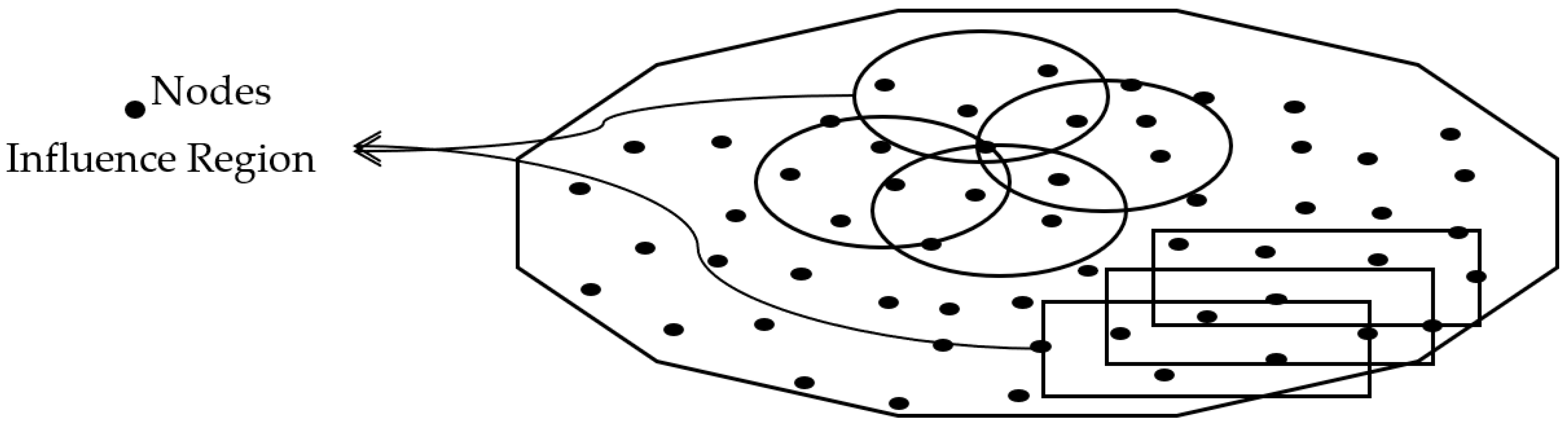
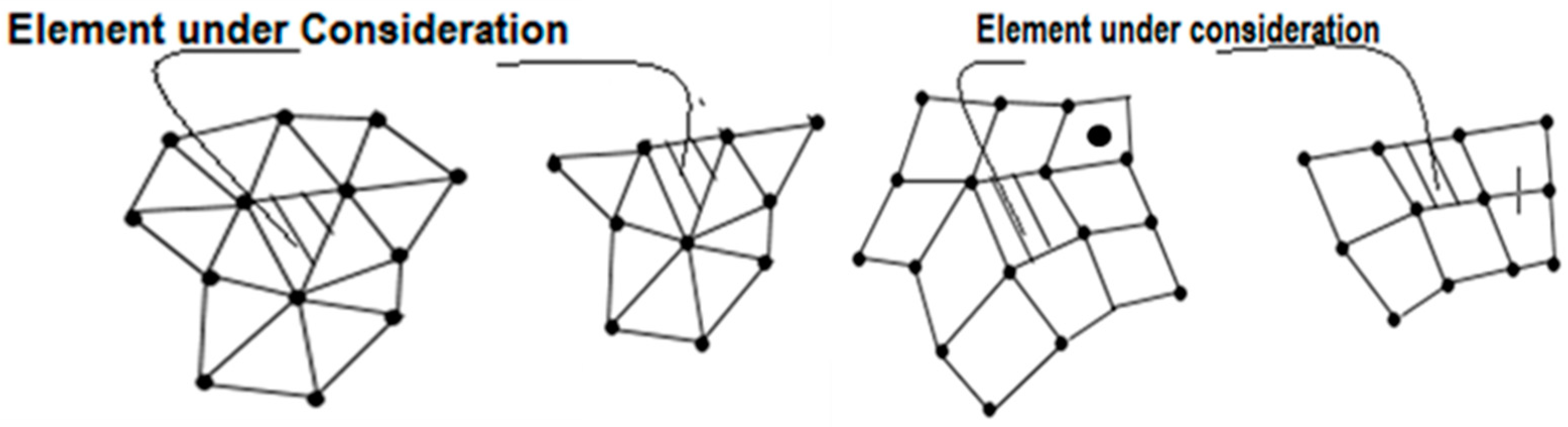
3.1. Influence Region Shapes in Moving Least Squares (MLS) Interpolation

The degree of precision of MLS approximation for the node of interest is dictated by the influence region shape (Figure 1). The circular shape of node influence regions is constructed using the distance $\overline{d}=x-x_i/d_m$. The distance (x − x_i) represents the node x to point x_i distance, and dm denotes the influence region dimension of node x_i. The influence region dimension for the ith node, d_mi, is determined as “d_mi = d_max c_i, where d_max represents the dilation index, and distance c_i is assessed by probing for adequate distances to neighboring nodes. For the formation of the node’s rectangular influence regions, the cartesian direction distances are found as $r_x=\Vert x-x_i\Vert /d_{mx}$ and $r_y=\Vert x-y_i\Vert /d_{my}$, in which d_mx = d_max c_xi and d_my = d_max c_yi. In the case of irregularly dispersed nodes, c_i can be considered the nodal spacing (average) within the influence region of x_i, whereas for regularly dispersed nodes, c_i is merely the adjacent node’s distance.

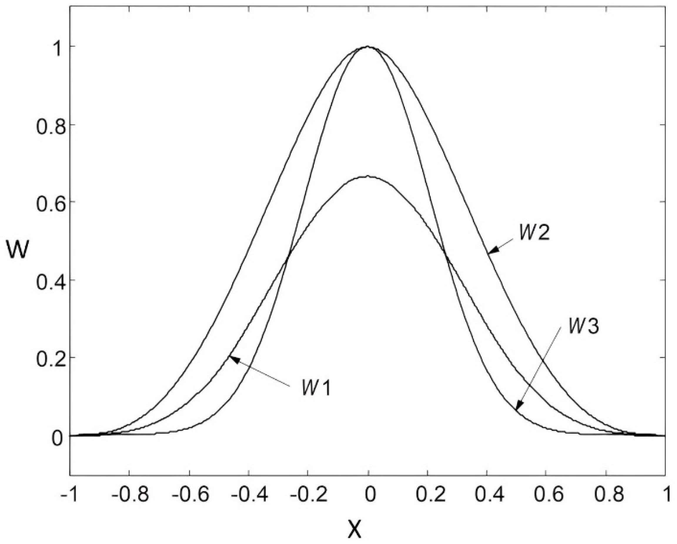
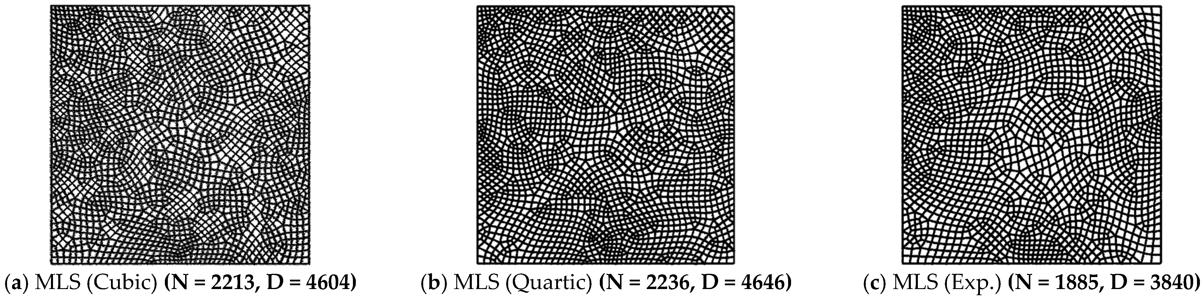
3.2. Weight Functions in Meshless MLS Interpolation

The weight function contributes significantly to the meshless MLS method performance. The meshless approaches allow for the use of various weight functions. The weights assume a value adjacent to the node as a unit where the function and its derivatives are to be computed and diminish beyond the subdomain area Ω_i neighboring the node x_i. The parametric study takes into account the following weight functions.

• Cubic Spline Functions (W1):

$$w\left(\overline{d}\right)=\left\{\begin{array}{cc}{\displaystyle \frac{2}{3}}-4{\overline{d}}^2+4{\overline{d}}^3& \mathrm{for} \overline{d} \le {\displaystyle \frac{1}{2}}\\ {\displaystyle \frac{4}{3}}-4\overline{d}+4{\overline{d}}^2-{\displaystyle \frac{4}{3}}{\overline{d}}^3& \mathrm{for} 1\le \overline{d} \le {\displaystyle \frac{1}{2}}\\ 0& \mathrm{for} \overline{d}>1\end{array}\right\},$$

(16)

• Quartic Spline Functions (W2):

$$w\left(\overline{d}\right)=\left\{\begin{array}{cc}1-6{\overline{d}}^2+8{\overline{d}}^3-3{\overline{d}}^4& \mathrm{for} \overline{d}\le 1\\ 0& \mathrm{for} \overline{d}>1\end{array}\right\},$$

(17)

• Exponential Functions (W3):

$$w\left(\overline{d}\right)=\left\{\begin{array}{cc}{e}^{-{({\displaystyle \frac{\overline{d}}{\alpha }})}^2}& \mathrm{for} \overline{d}\le 1\\ 0& \mathrm{for} \overline{d}>1\end{array}\right\},$$

(18)

Higher weights are given to node x_i that are near to x, and lower weights are given to nodes that are far from x. For optimal performance, the value of α is taken as 0.4. Figure 2 illustrates the variation of considered weight functions within the influence region.

4. Least Squares Interpolation for Displacement Recovery

Employing higher-order polynomial and mesh-based-node patches, the least square (LS) interpolation method is used to recover the displacement errors from the computed nodal displacement (Figure 3) [40].

$$u^h\left(x\right)={{\displaystyle \sum }}_{I=1}^n{{\displaystyle \sum }}_{j=1}^m{p}_j\left(x\right)A^{-1}\left(x\right)B{\left(x\right)}_{jI}{u}_I,$$

(19)

By minimizing the following functional, the least squares approximation of u^h across the mesh-dependent patches of a node can be found in the following manner,

$$u^h\left(x\right)={{\displaystyle \sum }}_{I=1}^n{{\displaystyle \sum }}_{j=1}^m{p}_j\left(x\right)A^{-1}\left(x\right)B{\left(x\right)}_{jI}{u}_I,$$

(20)

The solution to Equation (20) for unknown parameter ‘a’ provides the following equation.

$$\mathit{A} \mathit{a}=\mathit{b},$$

(21)

where $\mathit{A}={{\displaystyle \sum }}_{i=1}^n{P}_i^T\left(x_i,y_i\right)P_i\left(x_i,y_i\right), \mathit{b}={{\displaystyle \sum }}_{i=1}^{np}{P}_i^T\left(x_i,y_i\right)u_i^h\left(x_i,y_i\right)$.

5. Finite Element Analysis Accuracy and Effectivity

The finite element (FE) solution error is the field variable or gradients obtained by FE analysis that differ from the projected field variable or gradients a posteriori results (or exact results). The errors in the FE solution are represented in norms such as energy or L₂-norms and may be defined as follows.

$${\Vert e\Vert }_E={\left[{{\displaystyle \int }}_{\Omega }{e}_{\sigma }^{*T}{D}^{-1}{e}_{\sigma }^{*}\mathrm{d}\Omega \right]}^{{\displaystyle \frac{1}{2}}},$$

(22)

$${\Vert e\Vert }_{L_2}={\left[{\displaystyle \int }{e}_{\sigma }^{*T}{e}_{\sigma }^{*}\mathrm{d}\Omega \right]}^{1/2},$$

(23)

Effectivity (θ), (=computed error/exact error), is a factor and refers to a criterion or measure used to assess if the precision of a solution improves as the mesh is refined. The finite element solution accuracy ($\eta$) is given by relation $\eta ={\displaystyle \frac{\Vert {\mathit{e}}^{\mathbf{*}}\Vert }{\Vert {\mathit{\sigma }}^{\mathbf{*}}\Vert }}$ in which ${\Vert {\sigma }^{*}\Vert }^2={\Vert {\sigma }^h\Vert }^2+{{\Vert e\Vert }_E}^2$. If the computational results accuracy falls short of the intended (permissible) level, the mesh can be updated optimally, focusing only on regions where errors exceed the intended threshold to minimize solution error. Techniques such as evenly distributing the solution error or its square across the mesh can be employed to update the mesh and achieve the desired accuracy level.

The permissible global error is found as follows.

$${\Vert e\Vert }_{permissible}={\eta }_{permissible}\Vert e\Vert /k,$$

(24)

where the value of k is between 1.0 and 1.5 to prevent oscillation [41].

For the square of the solution error for the evenly distributed strategy, the permissible error in the ith element can be found as follows.

$${\Vert e\Vert }_{permissible\left(i\right)}={\eta }_{permissible}{\left({\displaystyle \frac{{\Omega }_i}{\Omega }}\right)}^{1/3},$$

(25)

The mesh modification in the primary mesh is required when the refinement parameter, ${\mathsf{\xi }}_i$, ($={\displaystyle \frac{{\Vert e\Vert }_{permissible}}{{\Vert e\Vert }_{permissible\left(i\right)}}}$) is greater than one. If the old mesh size is kept, then the new mesh size (h_new) can be calculated by employing the following relation.

$$h_{new}={\displaystyle \frac{h_{new}}{{\mathsf{\xi }}_i^{1/m}}},$$

(26)

The methodology following the above-mentioned formulations for meshless error recovery incorporating an adaptive analysis of incompressible elastic problems is presented in a flow chart (Figure 4) and implemented in Fortran-based software (Figure 5).

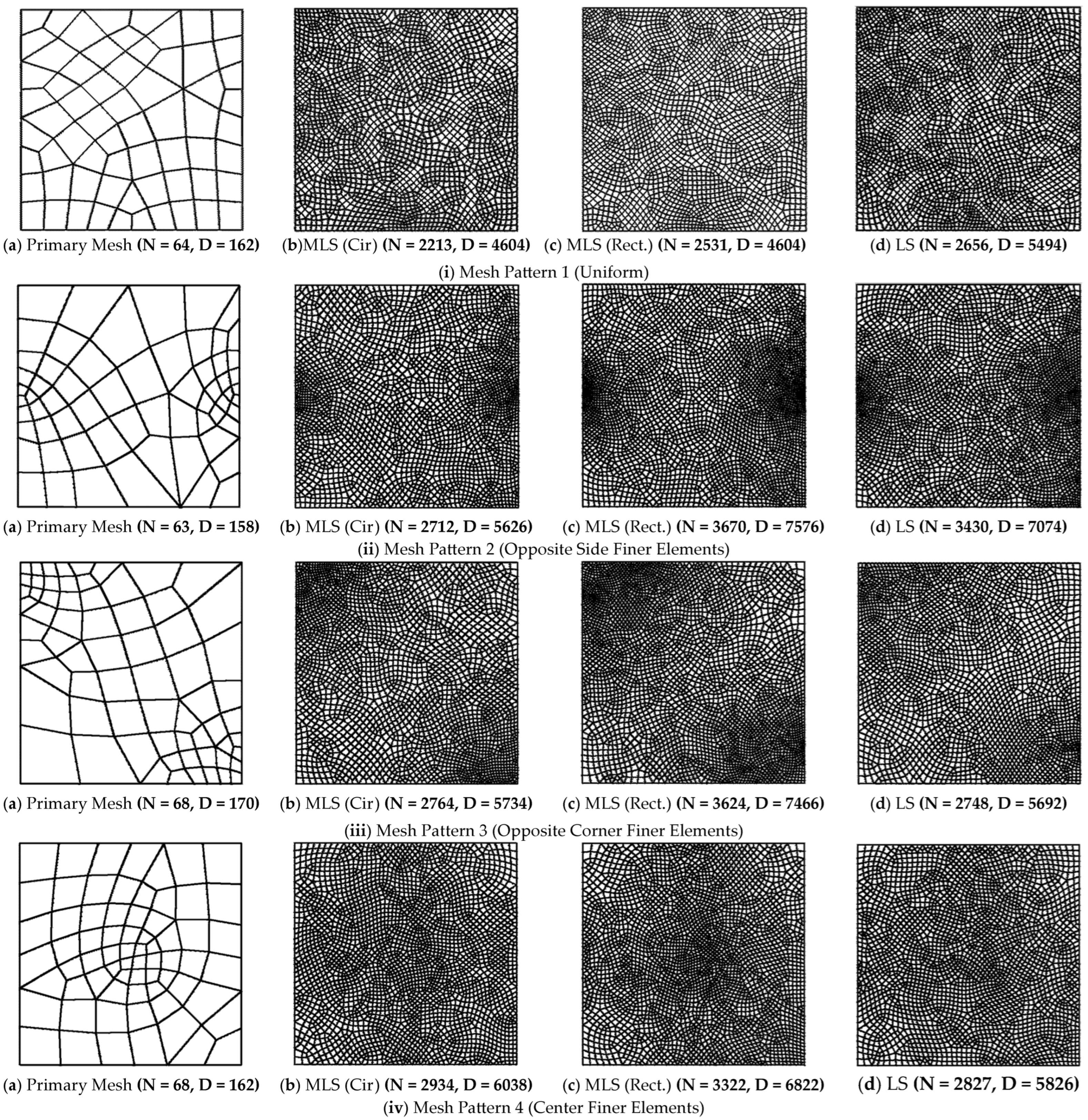
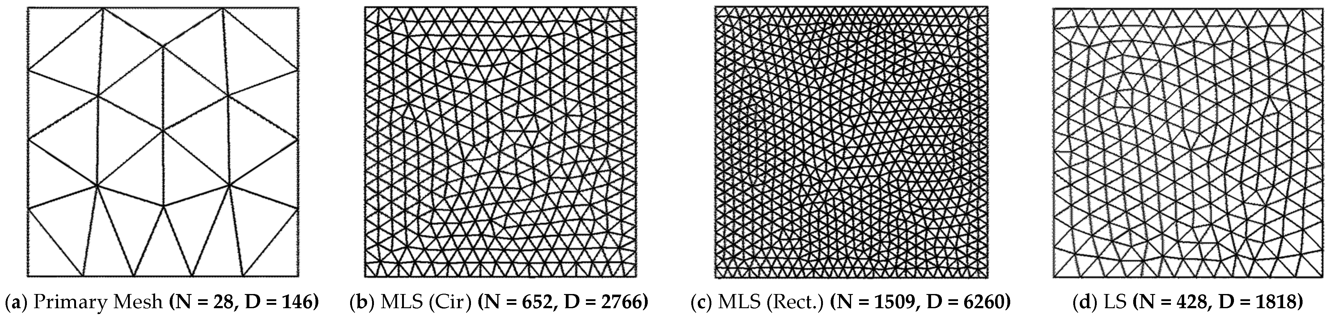
6. Parametric Investigation of Meshless Error Recovery Procedures

An analysis of incompressible elastic benchmark plate problems is conducted to explore recovery parameters influencing error evaluation, including effectivity, error convergence rate, and updated domain discretization. The incompressibility of the problem is dealt with mixed finite formulation and reduced integration for volumetric strain terms, considering one-point reduced integration with quadrilateral elements (4-node) and two-point reduced integration with triangular elements (6-node) for volumetric strain terms. The incompressible elasticity plates are discretized utilizing the four-node quadrilaterals and six-node triangular meshes. The computational errors (local and global) are computed in terms of energy and L₂-norm. The quality of interpolation-type error recovery procedures is studied by varying recovery factors such as types of interpolation schemes, size/configuration of the patch for interpolation, error norm, meshing schemes, mesh patterns, and weight function. The circular/rectangular configuration influence regions are employed in the meshless MLS interpolation approach. The element-based patch of a node is employed for the LS interpolation approach. This study considers cubic spline, quartic spline, as well as exponential weight functions in order to extract the solution errors employing quadrilateral and triangular meshing, respectively.

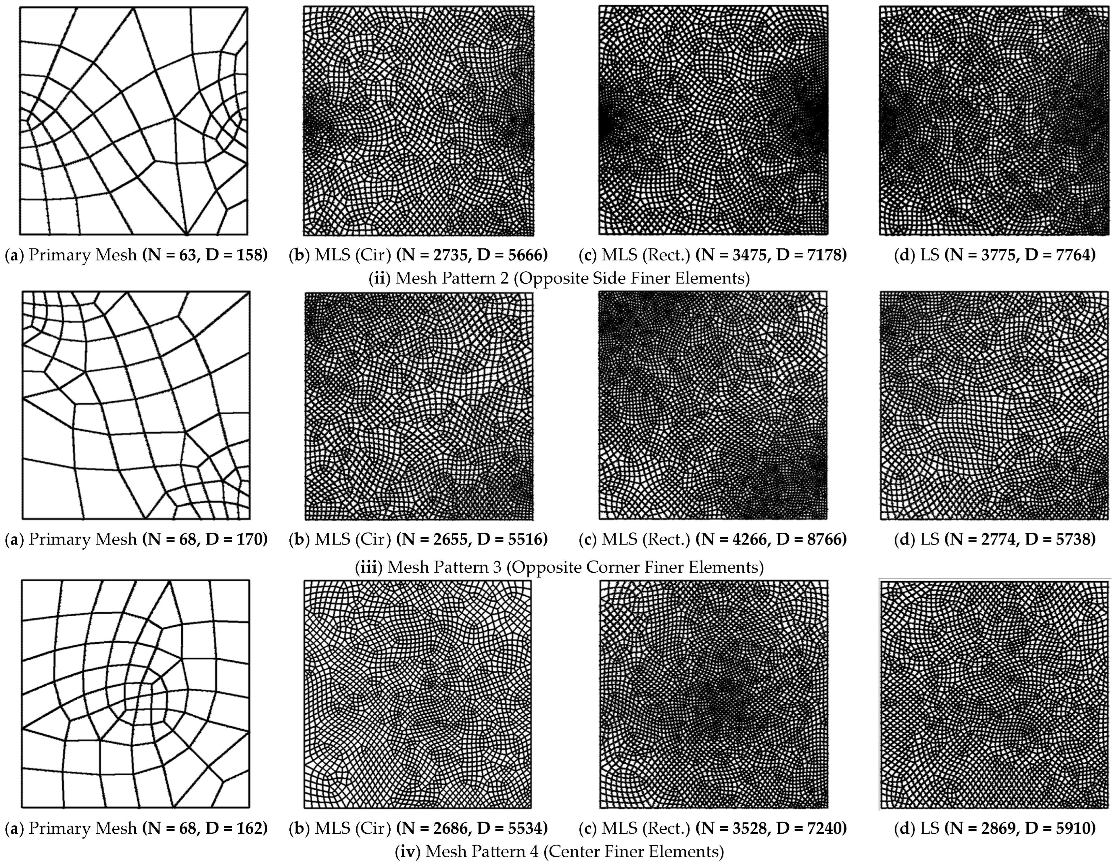
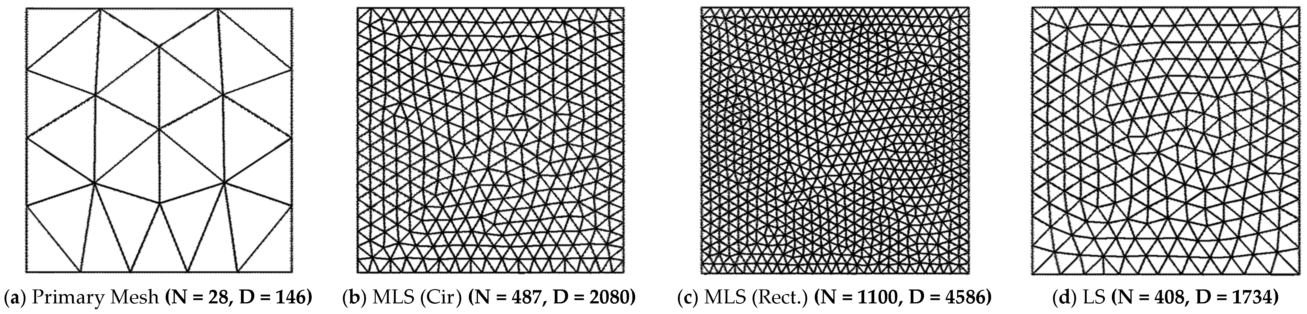
6.1. Finite Element Method-Based Analysis of Incompressible Elastic Plate

The analysis of the illustrative example of a plate, under the influence of body forces (b_x, b_y) (Equations (33)–(34)) and under the constraints of incompressible elasticity assesses the impact of recovery factors on error estimation through the finite element technique. The plate body forces are stated in terms of polynomials. The analytical displacements (u, v) and strains (ε_x, ε_y, ε_xy) from the application of body forces are given in Equations (27)–(33) [37]. The problem domain with quadrilateral and triangular meshing is shown in Figure 6.

• Problem Domain = Ω [0 × 0] × [1 × 1], u = v = 0 on Γ
• Exact solution for Displacements

$$u=2x^{2}y{\left(1-x\right)}^2\left(1-y\right)\left(1-2y\right),$$

(27)

$$v=-2x y^2\left(1-x\right)\left(1-2x\right) {\left(1-y\right)}^2,$$

(28)

• Exact solution for Strains

$${\epsilon }_x=\mathrm{y}\left(1-y\right)\left(1-2y\right)\left(4x+8x^3-12x^2\right),$$

(29)

$${\epsilon }_y=-x\left(1-x\right)\left(1-2x\right)\left(4y+8y^3-12y^2\right),$$

(30)

$${\epsilon }_{xy}=2x^2{\left(1-x\right)}^2 \left(1-6y+6y^2\right)+2y^2{\left(1-y\right)}^2 \left(-1+6x-6x^2\right),$$

(31)

• Body Forces

$$w_x=4y \left(1-6x+6x^2\right)\left(1-3y+2y^2\right)+12x^2\left(1-2x+x^2\right)\left(-1+2y\right)-2x,$$

(32)

$$w_y=-4x\left(1-6y+6y^2\right)\left(1-3x+2x^2\right)+12y^2\left(1-2y+y^2\right)\left(-1+2x\right)+2y,$$

(33)

Recovery Parameters: Interpolation Procedure Type, Mesh Pattern, Patch/Influence Region Configuration, Weight Functions and Error Norms

This study determines the impact of error recovery parameters on the effectivity and efficiency of the MLS interpolation by varying the size and arrangement of influence regions, weight functions and error norms. The MLS interpolation technique uses circular and rectangular shapes for the influence region, as formed in Figure 1. The patch of nodes for LS interpolation involves nodes of all the elements that surround the element being considered, as shown in Figure 3. The influence of interpolation formulation on error recovery results is explored while maintaining a dilation index of 3.0 for quadrilateral elements and the circular/rectangular shape influence region, while for quadratic triangular elements, the dilation index is 7.5 for the circular shape influence region and 5.0 for the rectangular shape influence region. The polynomial order of basis function is set to six for linear quadrilateral elements and nine for quadratic triangular elements.

Table 1. Recovered displacement errors (Energy Norm) and effectivity (θ) for plate problem with interpolation-type procedures utilizing linear quadrilateral element.

(a) Structured Mesh
Mesh Size (1/h)		Exact Error (×10−2)	MLS-Based Recovered Error [dmax= 3.0, m = 6]								LS-Based Recovered Error
			Cubic Spline				Quartic Spline		Exponential
			Circular Influence Region		Rectangular Influence Region		Circular Influence Region		Circular Influence Region		Element-Based Patch
			Error (×10−2)	θ	Error (×10−2)	θ	Error (×10−2)	θ	Error (×10−2)	θ	Error (×10−2)	θ
1/4		29.444	22.733	0.8210	40.169	1.1796	17.907	0.8263	17.708	0.5927	19.800	0.9173
1/8		15.256	4.635	0.9034	12.753	1.0836	3.512	0.9332	5.439	0.8273	7.036	0.9917
1/16		7.693	0.934	0.9703	2.555	0.9857	0.729	0.9806	1.472	0.9424	2.131	1.0019
1/32		3.855	0.197	0.9917	0.483	0.9910	0.159	0.9946	0.387	0.9835	0.589	1.0013
Conv. Rate		0.9777	2.2847		2.1261		2.2681		1.8389		1.6900
(b) Unstructured Mesh
Irregular Mesh Detail		Exact Error (×10−2)	MLS-Based Recovered Error [Cubic Spline, dmax = 3.0, m = 6]								LS-Based Recovered Error
			Cubic Spline				Quartic Spline		Exponential
			Circular Influence Region		Rectangular Influence Region		Circular Influence Region		Circular Influence Region		Element-Based Patch
Element Numbers	Degree of Freedom		Error (×10−2)	θ	Error (×10−2)	θ	Error (×10−2)	θ	Error (×10−2)	θ	Error (×10−2)	θ
16	50	29.449	15.853	0.8187	33.670	0.9813	18.101	0.8353	18.204	0.4925	19.795	0.9173
64 a	162	17.999	8.837	0.8727	8. 999	0.9311	9.512	0.9442	10.543	0.7511	11.469	0.9695
63 b	158	26.627	24.793	1.0273	16.475	1.0272	-	-	-	-	17.991	0.9252
68 c	170	23.107	27.896	1.4885	16.659	1.0007	-	-	-	-	13.314	0.9942
68 d	162	22.445	14.165	0.7617	19.181	0.8410	-	-	-	-	15.884	0.8571
282	630	8.463	2.264	0.9525	2.312	0.9677	3.729	0.9701	5.273	0.8926	3.063	0.9907
1212	2566	3.673	0.726	0.9825	0.544	0.9883	0.859	0.9812	0.995	0.9137	0.723	1.0025

^a Mesh pattern 1 (uniform); ^b mesh pattern 2 (plate opposite side finer elements); ^c mesh pattern 3 (plate opposite corner finer elements); ^d mesh pattern 4 (plate center finer elements).

,

Table 2. Recovered displacement errors (energy norm) and effectivity (θ) for plate problem with interpolation-type procedures utilizing quadratic triangular element.

(a) Structured Mesh
Mesh Size (1/h)		Exact Error (×10−2)	MLS-Based Recovered Error [m = 9]								LS-Based Recovered Error
			Cubic Spline				Quartic Spline		Exponential
			Circular Influence Region [dmax = 7.5]		Rectangular Influence Region [dmax = 5]		Circular Influence Region [dmax = 7.5]		Circular Influence Region [dmax = 7.5]		Element-Based Patch
			Error (×10−2)	θ	Error (×10−2)	θ	Error (×10−2)	θ	Error (×10−2)	θ	Error (×10−2)	θ
1/4		40.201	23.896	1.0136	30.462	1.0768	25.733	1.0351	33.437	0.6657	19.073	0.9328
1/12		14.110	2.280	0.9879	3.038	0.9994	2.429	0.9902	11.556	0.7101	2.258	0.9663
1/24		7.025	0.568	0.9929	0.652	0.9952	0.584	0.9938	788.54	112.236	0.683	0.9720
Conv. Rate		0.9736	2.0869		2.1452		2.1128		1.7639		1.8578
(b) Unstructured Mesh
Irregular Mesh Detail		Exact Error (×10−2)	MLS-Based Recovered Error [Cubic Spline, m = 9]								LS-Based Recovered Error
			Cubic Spline				Quartic Spline		Exponential
			Circular Influence Region [dmax = 7.5]		Rectangular Influence Region [dmax = 5]		Circular Influence Region [dmax = 7.5]		Circular Influence Region [dmax = 7.5]		Element-Based Patch
Element Numbers	Degree of Freedom		Error (×10−2)	θ	Error (×10−2)	θ	Error (×10−2)	θ	Error (×10−2)	θ	Error (×10−2)	θ
28	146	35.233	29.014	0.4241	33.854	0.6655	26.644	0.9821	35.354	0.7358	28.856	0.5690
291	1264	7.085	2.085	0.9455	2.583	0.9418	5.617	0.9876	13.556	0.8001	3.264	0.8541
1149	4792	2.805	0.628	0.9529	0.719	0.9380	0.846	0.9912	-	-	1.110	0.8838

,

Table 3. Recovered displacement errors (L₂-norm of stress) and effectivity (θ) for plate problem with interpolation-type procedures utilizing linear quadrilateral element.

(a) Structured Mesh
Mesh Size (1/h)		Exact Error (×10−2)	MLS-Based Recovered Error [Cubic Spline, dmax = 3.0, m = 6]				LS-Based Recovered Error
			Circular Influence Region		Rectangular Influence Region		Element-Based Patch
			Error (×10−2)	θ	Error (×10−2)	θ	Error (×10−2)	θ
1/4		32.216	29.485	0.8335	49.214	1.2418	26.653	0.9312
1/8		16.525	5.725	0.8887	16.448	1.1467	9.668	0.9950
1/16		8.315	1.135	0.9667	3.183	0.9869	2.918	1.0026
1/32		4.164	0.242	0.9909	0.592	0.9900	0.805	1.0015
Conv. Rate		0.9838	2.3092		2.1258		1.6829
(b) Unstructured Mesh
Irregular Mesh Detail		Exact Error (×10−2)	MLS-Based Recovered Error [Cubic Spline, dmax = 3.0, m = 6]				LS-Based Recovered Error
			Circular Influence Region		Rectangular Influence Region		Element-Based Patch
Element Numbers	Degree of Freedom		Error (×10−2)	θ	Error (×10−2)	θ	Error (×10−2)	θ
16	50	32.219	20.592	0.7850	41.020	1.0132	26.647	0.9312
64 a	162	21.671	10.796	0.8864	11.327	0.9471	15.365	0.9966
63 b	158	32.080	29.993	1.0440	20.331	0.9071	23.042	0.9318
68 c	170	26.699	37.512	1.6384	20.977	1.0402	17.933	1.0151
68 d	162	25.639	16.879	0.7708	22.867	0.8531	20.828	0.8736
282	630	10.147	2.792	0.9593	2.861	0.9747	4.136	0.9996
1212	2566	4.159	0.892	0.9800	0.672	0.9862	0.956	1.0011

^a Mesh pattern 1 (uniform); ^b mesh pattern 2 (plate opposite side finer elements); ^c mesh pattern 3 (plate opposite corner finer elements); ^d mesh pattern 4 (plate center finer elements).

and

Table 4. Recovered displacement errors (L₂-norm of stress) and effectivity (θ) for plate problem with interpolation-type procedures utilizing quadratic triangular element.

(a) Structured Mesh
Mesh Size (1/h)		Exact Error (×10−2)	MLS-Based Recovered Error [Cubic Spline, m = 9]				LS-Based Recovered Error
			Circular Influence Region [dmax = 7.5]		Rectangular Influence Region [dmax = 5.0]		Element-Based Patch
			Error (×10−2)	θ	Error (×10−2)	θ	Error (×10−2)	θ
¼		46.782	29.667	1.0381	36.656	1.1024	23.437	0.9420
1/16		16.128	2.817	0.9904	3.833	1.0058	2.642	0.9647
1/24		8.056	0.693	0.9930	0.814	0.9963	0.795	0.9707
Conv. Rate		0.9818	2.0964		2.1244		1.8885
(b) Unstructured Mesh
Irregular Mesh Detail		Exact Error (×10−2)	MLS-Based Recovered Error [Cubic Spline, m = 9]				LS-Based Recovered Error
			Circular Influence Region [dmax = 7.5]		Rectangular Influence Region [dmax = 5.0]		Element-Based Patch
Element Numbers	Degree of Freedom		Error (×10−2)	θ	Error (×10−2)	θ	Error (×10−2)	θ
28	146	39.720	23.854	0.6655	28.604	0.7096	33.072	0.6024
291	1264	7.721	2.685	0.9671	3.303	0.9680	3.444	0.8639
1149	4792	3.109	0.715	0.9611	0.790	0.9466	1.172	0.8913

present the computational results, including error convergence (energy and L₂-norms) and global effectivity, obtained using LS and meshless MLS interpolation-based error extraction techniques with three weight functions for quadrilateral/triangular elements with structured/non-structured domain discretization, respectively. The results also include the finite element analysis errors and effectivity of errors with four different mesh patterns, namely, uniform mesh in plate, finer element mesh on opposite sides of plate, finer element mesh on opposite corner of plate and finer element mesh at plate center (Table 1b and Table 3b). Additionally, the local (element) effectivity frequency within the discretized elements in the plate domain is presented for recovery factors. Plots of local (element) effectivity frequency obtained when the problem is meshed utilizing linear quadrilateral/quadratic triangular elements, considering the circular/rectangular influence region used in meshless MLS interpolation-based and least square interpolation recovery techniques at a maximum mesh density, are given in Figure 7, Figure 8 and Figure 9 for energy and L₂-norms, respectively. The adaptive analysis in which initial meshes are improved for intended accuracy, with varying recovery parameters and with feedback from the error estimation, is also carried out. The improved meshes with an intended accuracy of 2% in energy norm and L₂-norm utilizing interpolation-based error assessments are depicted in Figure 10, Figure 11, Figure 12, Figure 13, Figure 14 and Figure 15 for quadrilateral and triangular meshing elements (N) and DOF (D) in improved meshes.

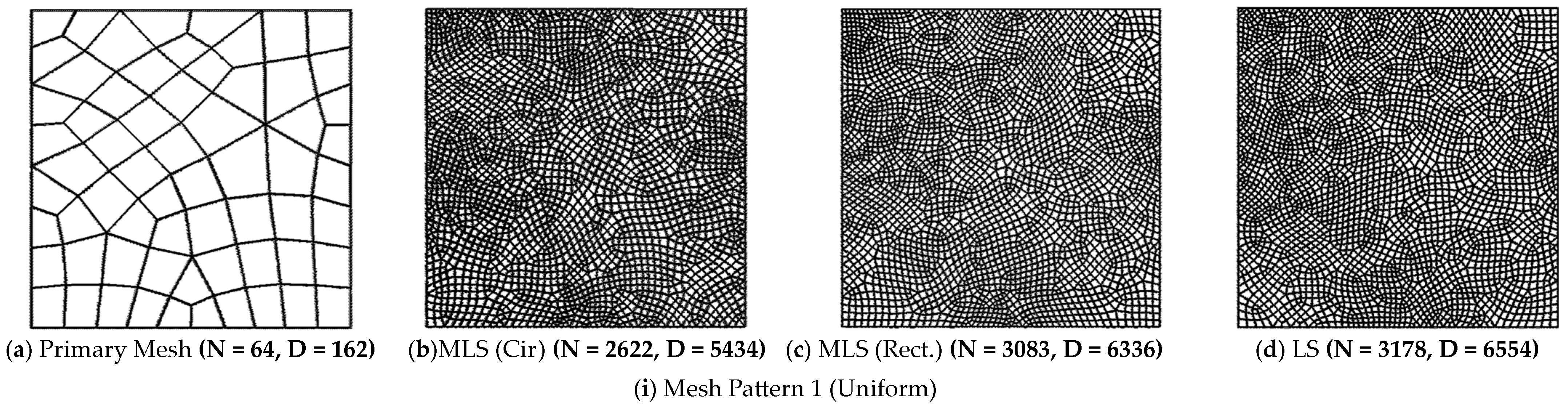
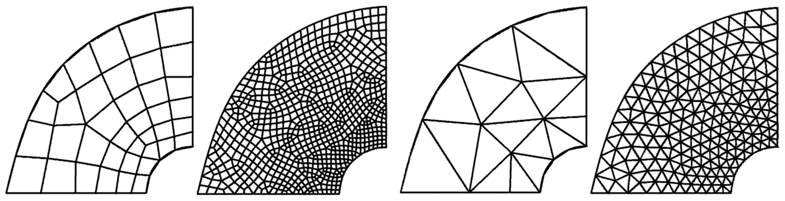
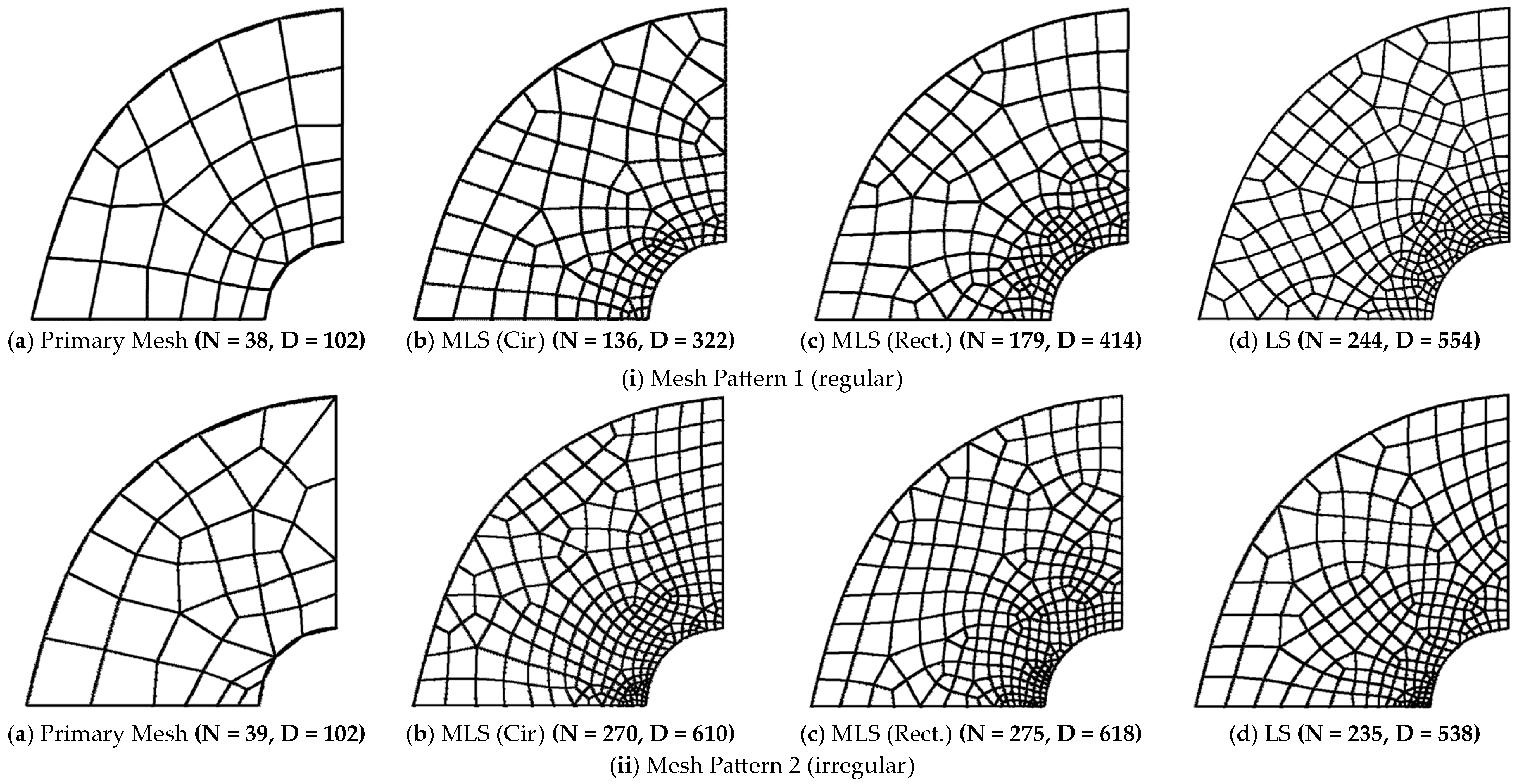
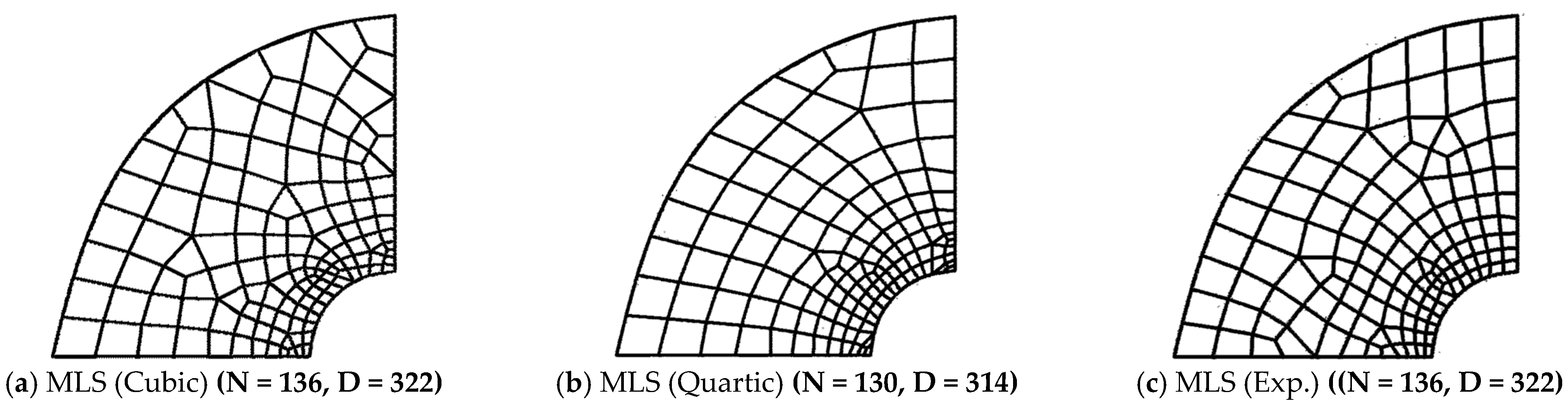
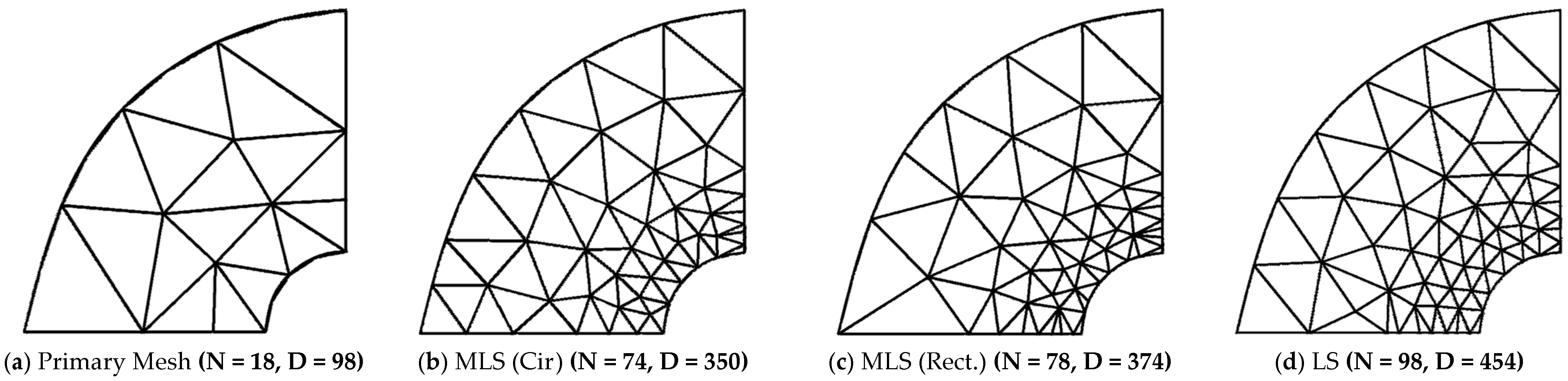
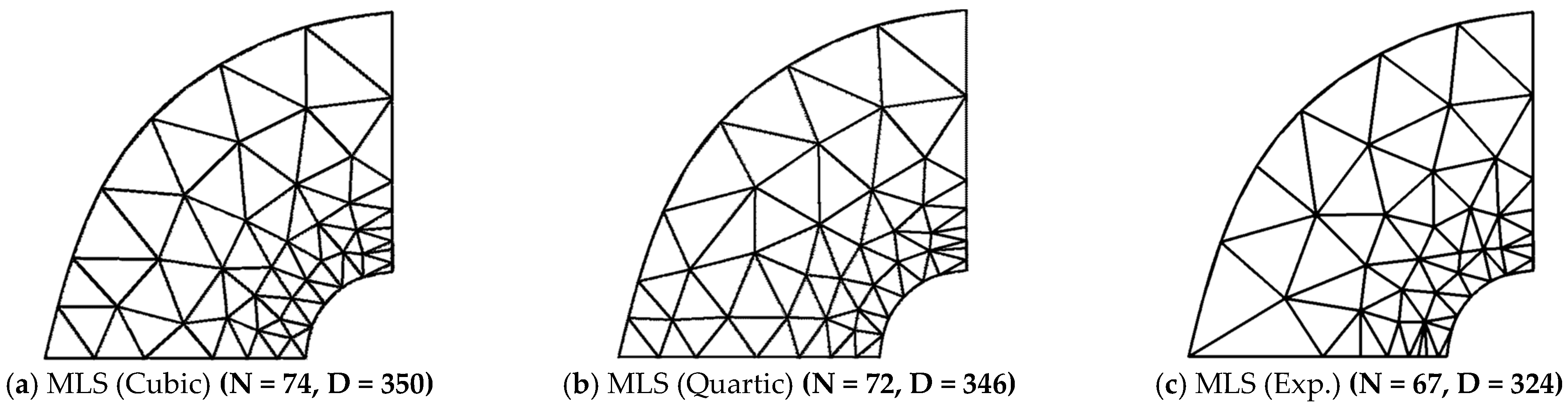
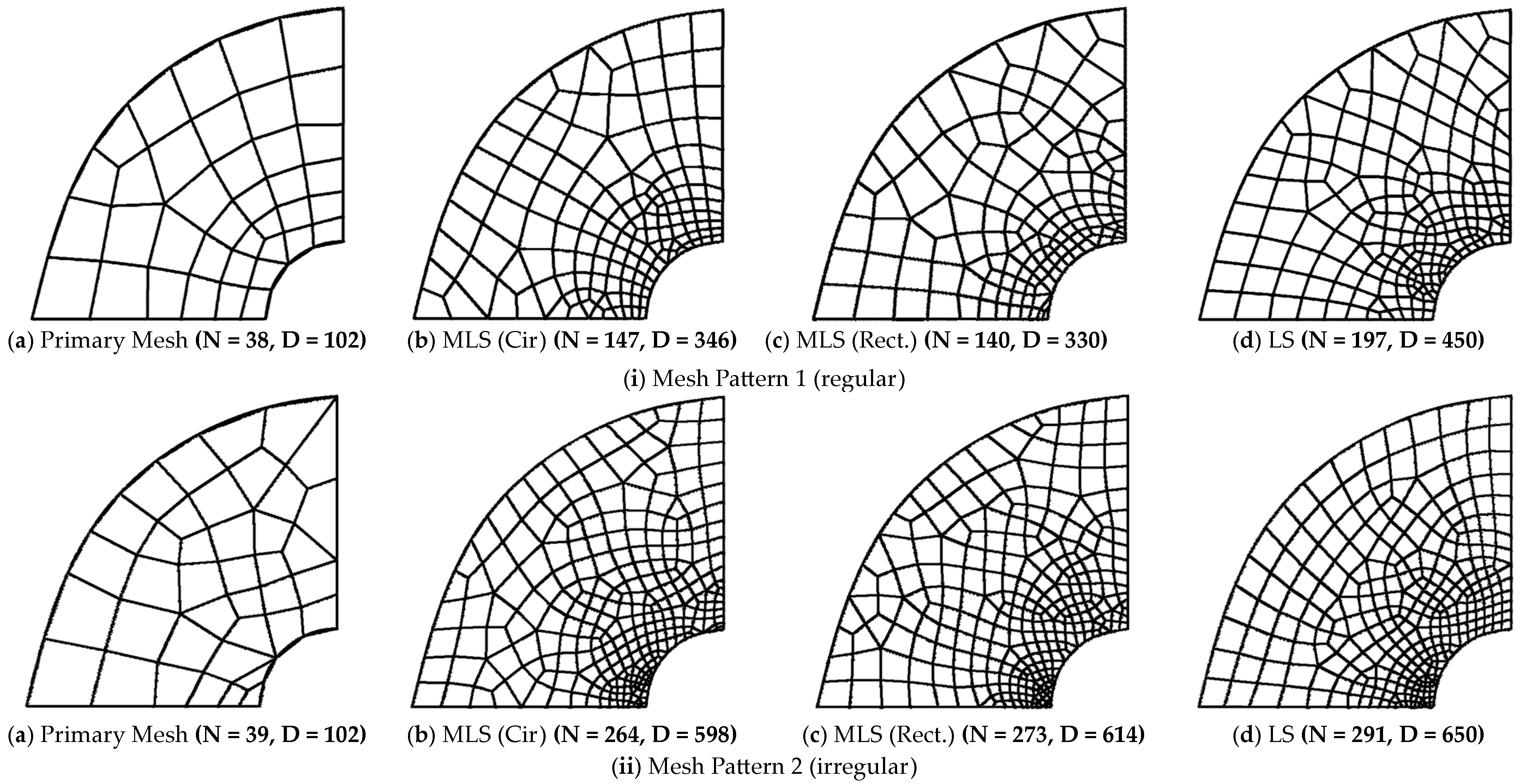
6.2. Finite Element Method-Based Analysis of Incompressible Elastic Cylinder Problem

The benchmark thick-walled cylinder problem is examined, evaluating error recovery properties using mesh-free MLS interpolation and LS interpolation error recovery techniques [42]. The cylinder is made of incompressible elastic material and assumes an in-plane strain condition. The inner radius and outer radius of the cylinder are r_i, and r_o, and the cylinder is subjected to internal pressure, p_i, and external pressure, p_o. The closed-form solution for exact displacements and stresses in the x and y directions is given by

$$u_x=\left({\displaystyle \frac{3}{2Er}}\right){(r_i r_o)}^2\left({\displaystyle \frac{p_i-p_o}{{r_o}^2-{r_i}^2}}\right)cos\theta ,$$

(34)

$$u_y=\left({\displaystyle \frac{3}{2Er}}\right){(r_i r_o)}^2\left({\displaystyle \frac{p_i-p_o}{{r_o}^2-{r_i}^2}}\right)sin\theta ,$$

(35)

$${\sigma }_{rr}={\displaystyle \frac{{( r_i r_o)}^2}{r^2}}\left({\displaystyle \frac{p_i-p_o}{{r_o}^2-{r_i}^2}}\right)+\left({\displaystyle \frac{p_{i }{r_i}^2-p_o{r_o}^2}{{r_o}^2-{r_i}^2}}\right),$$

(36)

$${\sigma }_{\theta \theta }=-{\displaystyle \frac{{( r_i r_o)}^2}{r^2}}\left({\displaystyle \frac{p_i-p_o}{{r_o}^2-{r_i}^2}}\right)+{\displaystyle \frac{p_{i }{r_i}^2-p_o{r_o}^2}{{r_o}^2-{r_i}^2}},$$

(37)

$${\sigma }_{r\theta }=0,$$

(38)

$${\sigma }_{xx}={\sigma }_{rr} co{s}^2\theta +{\sigma }_{\theta \theta } si{n}^2\theta ,$$

(39)

$${\sigma }_{yy}={\sigma }_{rr} si{n}^2\theta +{\sigma }_{\theta \theta } co{s}^2\theta ,$$

(40)

$${\sigma }_{xy}=\left({\sigma }_{\theta \theta }-{\sigma }_{rr}\right) cos\theta sin\theta ,$$

(41)

The cylinder problem considers outer radius (r_o) and inner radius (r_i) as 0.5 and 2 units. The cylinder is under an outer pressure (p_o) of 1 kN/mm² and internal pressure (p_i) of 2 kN/mm². The cylinder domains (quarter parts due to symmetry) are meshed with linear quadrilateral and quadratic triangular elements, as depicted in Figure 16.

Recovery Parameters: Interpolation Procedure Type, Mesh Pattern, Patch/Influence Region Configuration, Weight Functions and Error Norms

To recover the field variable error, the effects of the influence region of the shape/nodes patch on meshless MLS and on least square (LS) interpolation are evaluated. The meshless MLS interpolation technique uses a circular influence region, as formed in Figure 1, while Figure 3 shows the node patch used in the least square interpolation. The dilation index with a value of 3.0 is used in the construction of the influence region. This study considers the term number in the polynomial expansion of the basis function as six for linear quadrilateral elements, while the term number in polynomial expansion is considered nine for quadratic triangular elements.

Table 5. Recovered displacement errors (energy norm) and effectivity (θ) for cylinder problem using various interpolation-type procedures and influence regions.

(a) Linear Quadrilateral Element
Irregular Mesh Detail		Exact Error (×10−2)	MLS-Based Recovered Error [m = 6]								LS-Based Recovered Error
			Cubic Spline				Quartic Spline		Exponential
			Circular Influence Region [dmax = 3.25]		Rectangular Influence Region [dmax = 2]		Circular Influence Region [dmax = 3.25]		Circular Influence Region [dmax = 3.25]		Element-based Patch
Element Numbers	Degree of Freedom		Error (×10−2)	θ	Error (×10−2)	θ	Error (×10−2)	θ	Error (×10−2)	θ	Error (×10−2)	θ
38 a	102	1.015	0.464	0.9258	0.612	0.9317	0.507	0.9296	0.566	0.7535	0.724	1.0015
39 b	102	1.338	0.784	1.0390	0.937	0.9533	-	-	-	-	1.160	1.0767
176	402	0.505	0.209	0.9325	0.216	0.9434	0.209	0.9419	0.220	0.8546	0.220	0.9704
766	1632	0.291	0.147	0.8915	0.174	0.8576	0.160	0.8386	0.191	0.8240	0.177	0.8850
(b) Quadratic Triangular Element
Irregular Mesh Detail		Exact Error (×10−2)	MLS-Based Recovered Error [m = 9]								LS-Based Recovered Error
			Cubic Spline				Quartic Spline		Exponential
			Circular Influence Region [dmax = 3.25]		Rectangular Influence Region [dmax = 2]		Circular Influence Region [dmax = 3.25]		Circular Influence Region [dmax = 3.25]		Element-Based Patch
Element Numbers	Degree of Freedom		Error (×10−2)	θ	Error (×10−2)	θ	Error (×10−2)	θ	Error (×10−2)	θ	Error (×10−2)	θ
18	98	0.840	0.740	1.1419	1.019	1.4419	0.601	1.0257	0.646	1.0661	1.059	1.5397
80	370	0.304	0.182	0.8379	0.210	0.9965	0.181	0.8587	0.243	0.8560	0.241	1.0241
357	1528	0.180	0.147	0.5910	0.155	0.4989	0.147	0.6133	0.171	0.4658	0.151	0.5532

^a mesh pattern 1 (regular); ^b mesh pattern 2 (irregular).

and

Table 6. Recovered displacement errors (L₂-norm of stress) and effectivity (θ) for cylinder problem with interpolation-type procedures utilizing quadratic triangular element.

(a) Linear Quadrilateral Element
Irregular Mesh Detail		Exact Error (×10−2)	MLS-Based Recovered Error [Cubic Spline, m = 6]				LS-Based Recovered Error
			Circular Influence Region [dmax = 3.0]		Rectangular Influence Region [dmax = 2.0]		Element-Based Patch
Element Numbers	Degree of Freedom		Error (×10−2)	θ	Error (×10−2)	θ	Error (×10−2)	θ
38 a	102	68.368	33.126	0.9541	41.137	0.9401	54.199	1.0568
39 b	102	88.855	54.112	1.0487	62.241	0.9719	70.458	1.0539
64	162	35.872	14.354	0.9372	15.434	0.9417	19.845	1.0126
1212	2566	20.326	10.750	0.8786	10.798	0.9862	11.774	0.8710
(b) Quadratic Triangular Element
Irregular Mesh Detail		Exact Error (×10−2)	MLS-Based Recovered Error [Cubic Spline, m = 9]				LS-Based Recovered Error
			Circular Influence Region [dmax = 3.15]		Rectangular Influence Region [dmax = 1.65]		Element-Based Patch
Element Numbers	Degree of Freedom		Error (×10−2)	θ	Error (×10−2)	θ	Error (×10−2)	θ
18	98	58.818	35.570	0.9931	50.773	1.1076	66.952	1.4173
80	370	21.981	13.278	0.8906	14.602	0.9348	16.109	0.9732
357	1528	12.909	10.654	0.5926	10.752	0.6139	10.426	0.6694

^a mesh pattern 1 (regular); ^b mesh pattern 2 (irregular).

present the computational outcome, effectivity (global) and rate of error convergence (energy norms and L2-norm) obtained utilizing LS, as well as meshless MLS interpolation-based error extraction for quadrilateral and triangular elements, respectively. The results also include the finite element analysis errors and effectivity of errors with two mesh patterns, namely regular and irregular mesh in a cylinder. The adaptive analysis through the error recovery feedback using a 2% intended accuracy is also carried out. Figure 17, Figure 18, Figure 19, Figure 20, Figure 21 and Figure 22 illustrate the results of adaptive analysis, showing the improved mesh details [total elements in mesh (N) and degrees of freedom (D)] for achieving accuracy in energy and L₂-norm of stress with linear quadrilateral and quadratic triangular mesh.

7. Discussion

This study presents a parametric evaluation of meshless displacement error extraction techniques in a finite element solution under incompressibility conditions. Various error recovery parameters, including interpolation scheme types, patch size/influence region configuration for interpolation, weight functions, dilation index, error norm, meshing schemes and mesh pattern are considered. The assessment involves evaluating the effectivity (both local and global) of error evaluation, the recovered error convergence rate with increasing mesh density in energy norm and L₂-norm, and the use of adaptively refined meshes to achieve intended accuracy. The computational results for two incompressible elasticity benchmark problems (incompressible elastic plate and cylinder) are obtained using adaptive finite element analysis considering meshless MLS/LS interpolation technique-based error estimation and presented in Table 1, Table 2, Table 3, Table 4, Table 5 and Table 6 and Figure 7, Figure 8, Figure 9, Figure 10, Figure 11, Figure 12, Figure 13, Figure 14, Figure 15, Figure 17, Figure 18, Figure 19, Figure 20, Figure 21 and Figure 22. The results also include the finite element analysis errors and effectivity of errors with four different mesh patterns, namely uniform mesh in plate, finer element mesh on opposite sides of plate, finer element mesh on opposite corner of plate and finer element mesh at plate center, and regular and irregular mesh in cylinder (Table 1, Table 2, Table 3, Table 5 and Table 6).

From Table 1, Table 2, Table 3 and Table 4, which show the results for error convergence and effectivity considering energy norm and L₂-norm with MLS (circular/rectangular influence region)/LS interpolation and linear quadrilateral/quadratic triangular meshing, it is observed that recovery factors, interpolation approaches, and patch/influence region construction has a noticeable effect on the performance of error recovery and error estimation feedback-adaptive analysis. The tables show that the error values achieved using the recovery technique are significantly smaller than the finite element solution error, and the rate of error convergence is also substantially greater than the FEM solution error as mesh density increases. The order of error is greater with the rectangular influence region and when the error is quantified in L₂-norm. The tables show that meshless MLS interpolation error recovery outperforms LS interpolation error recovery, with higher error convergence rates and effectivity that approaches one. When comparing the recovery parameters of meshless MLS interpolation error recovery, i.e., meshing scheme, influence region shapes and error norms, the appreciable difference is not observed in convergence rates and global effectivity with the use of linear quadrilateral or quadratic triangular meshing, circular or rectangular influence regions and energy norm or L₂-norm. The local effectivity frequency for quadrilateral/quadratic triangular meshing in the energy/L₂-norm used in mesh-free MLS interpolation-based recovery techniques with circular/rectangular influence region shapes is plotted in Figure 7, Figure 8 and Figure 13 at the maximum mesh density considered. The figures show that in comparison to lower-order elements, higher-order elements and unstructured discretization are more sensitive to the influence-region shape type. It is evident from the error recovery results with various mesh patterns, as shown in Table 1, Table 3, Table 5 and Table 6, that the performance of error recovery is very much affected by the mesh patterns (distribution of elements in domains), and the MLS interpolation approach with the rectangular influence region is the most sensitive to the mesh pattern. It is also observed that error recovery performance is similar to the least squares and MLS interpolation approach at low mesh density.

Adaptive computational results for LS interpolation error recovery and meshless MLS interpolation error recovery (circular/rectangular influence regions) and various weight functions for the plate problem are depicted in Figure 9, Figure 10, Figure 11 and Figure 12, Figure 14 and Figure 15, respectively, utilizing quadrilateral/quadratic triangular meshing for domain discretization. These figures present the total elements in mesh (N) and degrees of freedom (DOF) in improved meshes necessary to maintain the intended accuracy of 2% in energy/L₂-norm. The error variation in the problem domain is also indicated, with more mesh density locations corresponding to more solution errors. The total number of elements generated in improved meshes using specific error techniques reflects the efficiency of the adaptive analysis. Compared to LS interpolation-based error assessment with quadrilateral element discretization, meshless MLS interpolation-based error assessment requires fewer elements in the improved mesh to maintain the intended accuracy. However, using quadratic triangular element discretization in meshless MLS interpolation-based error estimation employing a rectangular influence and LS interpolation-based error assessment, the number of elements in improved meshes is higher. In conclusion, meshless MLS interpolation-based error estimation employing a circular influence region for interpolation demonstrates greater efficiency and a more faithful recovery of errors in the problem domain, regardless of domain discretization, error norms and mesh patterns.

It is also observed from the tables and figures that error order in the energy norm found in the finite element analysis using a linear quadrilateral element is lowest when employing an exponential weight function. However, the lowest error convergence and effectiveness away from unity are obtained with a quadratic triangular element and exponential weight function. The optimized mesh for an intended accuracy limit of 2% is obtained with an exponential weight function. The results conclude that the quality of the meshless MLS interpolation extraction technique is more effective and efficient with a cubic spline weight function in the incompressible elasticity problem.

To recover the errors in displacement, the effects of the influence region shape/node patches, mesh patterns and weight functions on the meshless MLS interpolation technique and LS interpolation are evaluated by analyzing incompressible elastic cylinders through the error-recovery coupled finite element technique. The error variation pattern in the problem domain is studied with the updated mesh for intended accuracy, consisting of different element densities at different locations of the cylinder domain. It is observed that the circular influencing region, the cubic spline weight function and a polynomial expansion are one order greater than that of the background meshing element, with the energy norm providing better performance than the MLS interpolation-based error recovery technique. The computational results obtained are more or less similar to the results of the incompressible elastic plate. It can be observed from the study that meshless MLS interpolation-based error estimation employing a circular influence region for interpolation, irrespective of domain discretization, mesh patterns and error norms, is more efficient and recovers errors in the problem domain more faithfully. The conclusion of the investigation is that for reducing finite element analysis errors, the structured mesh pattern with suitable discretization schemes is preferred. The study also concludes that a lower dilation index value with a rectangular influence region is preferred in regular meshes, and a higher dilation index value with a radial influence region is preferable to relatively irregular meshes of lower-order elements for improved MLS-based meshless error-estimator performance.

Recommendations for Future Study

Even though, meshless error recovery techniques are particularly well-suited for the finite element method due to their flexibility and ability to handle complex geometries, fracture conditions, and large deformations, meshless error recovery techniques have concerns, including applicability to nonlinear problems and time-dependent applications. For highly nonlinear and dynamic problems, meshless error recovery techniques require careful selection of shape functions for convergence and stability. Further study should focus on the challenges of nonlinear and time-dependent applications along with their computational expense for such problems. Based on the experience gained from the above meshless error estimation study, it is recommended that a thorough error and convergence analysis for specific applications should be conducted to address the specific challenges of meshless error recovery techniques in specific applications, and standard benchmark problems should be developed to evaluate the performance of meshless error recovery techniques.

8. Conclusions

This study conducts a parametric assessment of meshless displacement extraction techniques in the finite element analysis of incompressible elasticity problems. The effects of various solution error recovery parameters, such as types of interpolation schemes, patch size/configuration for interpolation, dilation index, weight functions, error norm and meshing schemes, are included in the study. It assesses error-recovery effectivity (local and global), convergence rates with refinement order in energy norm and L₂-norm, and adaptive mesh improvement for intended accuracy. The meshless moving least squares (MLS) interpolation procedure using rectangular/circular support regions and the least square interpolation procedure using element-based node patch are employed for finite element displacement solution error recovery. The benchmark two-dimensional plate and cylinder problems with incompressible conditions are analyzed using linear quadrilateral/quadratic triangular elements to investigate the influence of various recovery parameters. It can be observed from the study that meshless MLS interpolation-based error estimation employing circular influence regions for interpolation, irrespective of domain discretization, mesh patterns and error norms, is more efficient and recovers errors in the problem domain more faithfully. The conclusion of the investigation is that to reduce finite element analysis errors, a structured mesh pattern with suitable discretization schemes and an MLS weight function is preferred. The study also concludes that a lower dilation index value with a rectangular influence region is preferred in regular meshes, and a higher dilation index value with a radial influence region is preferable to relatively irregular meshes of lower-order elements for improved MLS-based meshless error estimator performance.

References

1. Dow, J.O. A Uniform Approach to the Finite Element Method and Error Analysis Procedures; Academic Press: Cambridge, MA, USA, 1999. [Google Scholar]
2. Cen, S.; Wu, C.J.; Li, Z.; Shang, Y.; Li, C. Some advances in high-performance finite element methods. Eng. Comput. 2019, 36, 2811–2823. [Google Scholar] [CrossRef]
3. Zeng, W.; Liu, G.R. Smoothed Finite Element Methods (S-FEM): An Overview and Recent Developments. Arch. Comput. Methods Eng. 2018, 25, 397–435. [Google Scholar] [CrossRef]
4. Farrell, P.E.; Gaticay, L.F.; Lamichhanez, B.; Oyarzúa, R.; Ruiz-Baier, R. Mixed Kirchhof stress-displacement—Pressure formulations for incompressible hyper elasticity. Comput. Methods Appl. Mech. Eng. 2021, 374, 113562. [Google Scholar] [CrossRef]
5. Boffi, D.; Stenberg, R. A remark on finite element schemes for nearly incompressible elasticity. Comput. Math. Appl. 2017, 74, 2047–2048. [Google Scholar] [CrossRef]
6. Rulff, P.; Buntin, L.M.; Kalscheuer, T. Efficient goal-oriented mesh refinement in 3-D finite-element modelling adapted for controlled source electromagnetic surveys. Geophys. J. Int. 2021, 227, 1624–1645. [Google Scholar] [CrossRef]
7. Nemer, R.; Larcher, A.; Coupez, T.; Hachem, E. Stabilized finite element method for incompressible solid dynamics using an updated Lagrangian formulation. Comput. Methods Appl. Mech. Eng. 2021, 384, 113923. [Google Scholar] [CrossRef]
8. Gültekin, O.; Dal, H.; Holzapfel, G.A. On the quasi-incompressible finite element analysis of anisotropic hyperelastic materials. Comput. Mech. 2019, 63, 443–453. [Google Scholar] [CrossRef]
9. Jiang, W.; Gao, X. Review of collocation methods and applications in solving science and engineering problems. Comput. Model. Eng. Sci. 2024, 140, 41–76. [Google Scholar] [CrossRef]
10. Lee, C.-K.; Mihai, L.A.; Hale, J.S.; Kerfriden, P.; Bordas, S.P.A. Strain smoothing for compressible and nearly-incompressible finite elasticity. Comput. Struct. 2017, 182, 540–555. [Google Scholar] [CrossRef]
11. Khan, A.; Powell, C.E.; Silvester, D.J. Robust a-posteriori error estimator for mixed approximation of nearly incompressible elasticity. Int. J. Numer. Methods Eng. 2019, 119, 18–19. [Google Scholar] [CrossRef]
12. Nikravesh, S.; Afshar, M.H.; Faraji, S. RPIM and RPIM-MLS-based MDLSM method for the solution to elasticity problems. Sci. Iran. Trans. A Civ. Eng. 2016, 23, 2458–2468. [Google Scholar] [CrossRef]
13. Ma, X.; Zhou, B.; Li, Y.; Xue, S. A Hermite interpolation element-free Galerkin method for elasticity problems. J. Mech. Mater. Struct. 2022, 17, 75–95. [Google Scholar] [CrossRef]
14. Ferro, N.; Perotto, S.; Cangiani, A. An Anisotropic Recovery-Based Error Estimator for Adaptive Discontinuous Galerkin Methods. J. Sci. Comput. 2022, 90, 45. [Google Scholar] [CrossRef]
15. Pagani, A.; Chiaia, P.; Filippi, M.; Cinefra, M. Unified three-dimensional finite elements for large strain analysis of compressible and nearly incompressible solids. Mech. Adv. Mater. Struct. 2024, 31, 117–137. [Google Scholar] [CrossRef]
16. Babuska, I.; Rheinboldt, W.C. A posteriori Error Estimator in Finite Element Method. Int. J. Numer. Methods Eng. 1978, 12, 1597–1615. [Google Scholar] [CrossRef]
17. Eriksson, K.; Johnson, C. An Adaptive Finite Element Method for Linear Elliptic Problems. Math. Comput. 1988, 50, 361–383. [Google Scholar] [CrossRef]
18. Zienkiewicz, O.C.; Zhu, J.Z. Simple error estimator and adaptive procedure for practical engineering analysis. Int. J. Numer. Methods Eng. 1987, 24, 337–357. [Google Scholar] [CrossRef]
19. Bramble, J.H.; Schatz, A.H. Higher Order Local Accuracy by Averaging in Finite Element Method. Math. Comput. 1977, 31, 94–111. [Google Scholar] [CrossRef]
20. Hinton, E.; Campbell, J.S. Local and Global Smoothing of Discontinuous Finite Element Functions using a Least Square Methods. Int. J. Numer. Methods Eng. 1974, 8, 61–80. [Google Scholar] [CrossRef]
21. Zienkiewicz, O.C.; Zhu, J.Z. The Super convergent Patch Recovery and a-posteriori Error Estimates, Part I, The Error Recovery Technique. Int. J. Numer. Methods Eng. 1992, 33, 1331–1364. [Google Scholar] [CrossRef]
22. Zienkiewicz, O.C.; Zhu, J.Z. The Super convergent Patch Recovery and a-posteriori Error Estimates. Part II: Error Estimates and Adaptivity. Int. J. Numer. Methods Eng. 1992, 33, 1365–1382. [Google Scholar] [CrossRef]
23. Rank, E.; Zienkiewicz, O.C. A Simple Error Estimator in The Finite Element Method. Commun. Appl. Numer. Methods 1987, 3, 243–249. [Google Scholar] [CrossRef]
24. Mirzaei, D. Analysis of Moving Least Squares Approximation Revisited. J. Comput. Appl. Math. 2015, 282, 237–250. [Google Scholar] [CrossRef]
25. Parret-Fréaud, A.; Rey, V.; Gosselet, P.; Rey, C. Improved recovery of admissible stress in domain decomposition methods—Application to heterogeneous structures and new error bounds for FETI-DP. Int. J. Numer. Methods Eng. 2016, 111, 69–87. [Google Scholar] [CrossRef]
26. Becker, R.; Gantner, G.; Innerberger, M.; Praetorius, D. Goal-oriented adaptive finite element methods with optimal computational complexity. Numer. Math. 2023, 153, 111–129. [Google Scholar] [CrossRef]
27. Pereira, J.T.; da Silva, J. Anisotropic Mesh Refinement Considering a Recovery-Based Error Estimator and Metric Tensors. Arab. J. Sci. Eng. 2019, 44, 5613–5630. [Google Scholar] [CrossRef]
28. Nie, Y.F.; Atluri, S.N.; Zuo, C.W. The Optimal Radius of the Support of Radial Weights Used in Moving Least Squares Approximation. Comput. Model. Eng. Sci. 2006, 12, 137–147. [Google Scholar]
29. Kahla, N.B.; AlQadhi, S.; Ahmed, M. Mesh-Free MLS-Based Error-Recovery Technique for Finite Element Incompressible Elastic Computations. Appl. Sci. 2023, 13, 6890. [Google Scholar] [CrossRef]
30. Perko, J.; Šarler, B. Weight Function Shape Parameter Optimization in Meshless Methods for Non-uniform Grids. Comput. Model. Eng. Sci. 2007, 19, 55–68. [Google Scholar]
31. Wang, J.G.; Liu, G.R. On the Optimal Shape Parameters of Radial Basis Functions used for 2-D Meshless Methods. Comput. Methods Appl. Mech. Eng. 2002, 191, 2611–2630. [Google Scholar] [CrossRef]
32. Kanber, B.; Bozkurt, O.Y.; Erklig, A. Investigation of RPIM Shape Parameter Effects on the Solution Accuracy of 2D Elastoplastic Problems. Int. J. Comput. Methods Eng. Sci. Mech. 2013, 14, 354–366. [Google Scholar] [CrossRef]
33. Hong, Y.; Ko, S.; Lee, J. Error analysis for finite element operator learning methods for solving parametric second-order elliptic PDEs. arXiv 2024, arXiv:2404.17868. [Google Scholar] [CrossRef]
34. Ahmed, M.; Singh, D.; Qadhi, S.A.; Thanh, N.V. Moving least squares interpolation-based a-posteriori error technique in finite element elastic analysis. Comput. Model. Eng. Sci. 2021, 129, 167–189. [Google Scholar] [CrossRef]
35. Mehraban, A.; Tufo, H.; Sture, S.; Regueiro, R. Matrix-free higher-order finite element method for parallel simulation of compressible and nearly-incompressible linear elasticity on unstructured meshes. Comput. Model. Eng. Sci. 2021, 129, 1283–1303. [Google Scholar] [CrossRef]
36. Lee, C.; Natarajan, S.; Hale, J.S.; Taylor, Z.A.; Yee, J.J.; Bordas, S. Bubble-enriched smoothed finite element methods for nearly-incompressible solids. Comput. Model. Eng. Sci. 2021, 127, 411–436. [Google Scholar] [CrossRef]
37. Zienkiewicz, O.C.; Lui, Y.C.; Huang, G.C. Error estimates and convergence rate for various incompressible elements. Int. J. Numer. Methods Eng. 1989, 28, 2192–2202. [Google Scholar] [CrossRef]
38. Onate, E.; Perazzo, F.; Miquel, J. A finite point method for elasticity problems. Comput. Struct. 2001, 79, 2151–2163. [Google Scholar] [CrossRef]
39. Liu, G.R.; Liu, M.B. Smoothed Particle Hydrodynamics—A Meshfree Particle Method; World Scientific Publishing Co. Pvt. Ltd.: Singapore, 2003. [Google Scholar] [CrossRef]
40. Ahmed, M. Techniques for Mesh Independent Displacement Recovery in Elastic Finite Element Solutions. Trans. Famena 2021, 45, 260308. [Google Scholar] [CrossRef]
41. Li, X.D.; Wiberg, N.E. A Posteriori Error Estimate by Element Patch Post-processing, Adaptive Analysis in Energy and L2 Norms. Comput. Struct. 1994, 53, 907–912. [Google Scholar] [CrossRef]
42. Coley, L.M.; Dolovich, A.T. Finite Element Calculations for incompressible Materials using a Modified LU Decomposition. Trans. Can. Soc. Mech. Eng. 2006, 30, 315–320. [Google Scholar] [CrossRef]
Figure 1. Influence region configuration for meshless MLS interpolation.
Mca 29 00087 g001
Figure 2. Weight Functions Variation in Influence Region [39].
Mca 29 00087 g002
Figure 3. Node patches (element connectivity) for LS interpolation.
Mca 29 00087 g003
Figure 4. Flow chart h-adaptive finite element procedure.
Mca 29 00087 g004
Figure 5. Partial source code.
Mca 29 00087 g005aMca 29 00087 g005b
Figure 6. Quadrilateral and triangular meshing in plate problem (structured and unstructured).
Mca 29 00087 g006
Figure 7. Frequency of element local effectivity (energy norm) in total No. of elements utilizing various influence region shapes in meshless MLS interpolation and LS recovery analysis.
Mca 29 00087 g007
Figure 8. Frequency of element local effectivity (energy norm) in total no. of elements utilizing various weight functions in meshless MLS interpolation and LS recovery analysis.
Mca 29 00087 g008
Figure 9. Frequency of element local effectivity (L2-norm of stress) in total no. of elements for plate problem (incompressible elastic) utilizing various configurations of influence region in mesh-free MLS interpolation recovery analysis.
Mca 29 00087 g009
Figure 10. Improved mesh detail for plate utilizing different configurations of influence region and primary mesh pattern [quadrilateral mesh, 2% intended accuracy, energy norm].
Mca 29 00087 g010
Figure 11. Improved mesh detail for plate utilizing different weight functions [quadrilateral uniform primary mesh (N = 64, D = 162), circular influence region, 2% intended accuracy, energy norm].
Mca 29 00087 g011
Figure 12. Primary mesh and improved mesh detail for plate utilizing different configurations of influence region [triangular mesh, 2% intended accuracy, energy norm].
Mca 29 00087 g012
Figure 13. Improved mesh detail for plate utilizing different weight functions [triangular uniform primary mesh (N = 28, D = 146), circular influence region, 2% intended accuracy, energy norm].
Mca 29 00087 g013
Figure 14. Improved mesh detail for Square Plate using various configurations of influence region and primary mesh pattern [quadrilateral mesh, 2% intended accuracy, L2-norm of stress].
Mca 29 00087 g014aMca 29 00087 g014b
Figure 15. Primary mesh and improved mesh detail for square plate using various configurations of influence region [triangular mesh, 2% intended accuracy, L2-norm of stress].
Mca 29 00087 g015
Figure 16. Quadrilateral and triangular meshing in cylinder problem.
Mca 29 00087 g016
Figure 17. Improved mesh detail for cylinder problem utilizing various configurations of influence region and primary mesh pattern [quadrilateral mesh, 2% intended accuracy, energy norm].
Mca 29 00087 g017
Figure 18. Improved mesh detail for plate utilizing different weight functions [quadrilateral uniform primary mesh (N = 38, D = 102), circular influence region, 2% intended accuracy, energy norm].
Mca 29 00087 g018
Figure 19. Primary mesh and improved mesh detail for cylinder problem utilizing various configurations of influence region [triangular mesh, 2% intended accuracy, energy norm].
Mca 29 00087 g019
Figure 20. Improved mesh detail for plate utilizing different weight functions [triangular uniform primary mesh (N = 18, D = 98), circular influence region, 2% intended accuracy, energy norm].
Mca 29 00087 g020
Figure 21. Improved mesh detail for cylinder problem utilizing various configurations of influence region and primary mesh pattern [quadrilateral mesh, 2% intended accuracy, L2-norm of stress].
Mca 29 00087 g021
Figure 22. Primary mesh and improved mesh detail for cylinder problem utilizing various configurations of influence region [triangular mesh, 2% intended accuracy, L2-norm of stress].
Mca 29 00087 g022