Abstract
The velocity and trajectory of particles moving along the corrugated (rough) surface under the action of gravity is obtained by a modified Method of Fundamental Solutions (MFS). This physical situation is found often in biological systems and microfluidic devices. The Stokes equations with no-slip boundary conditions are solved using the Green’s function for Stokeslets. In the present study, the velocity of a moving particle under the action of the gravity force is not known and becomes a part of the MFS solution. This requires an adjustment of the matrix of the MFS linear system to include the unknown particle velocity and incorporate in the MFS the balance of hydrodynamic and gravity forces acting on the particle. The study explores the combination of the regularization of Stokeslets and placement of Stokeslets outside the flow domain to ensure the accuracy and stability of computations for particles moving in proximity to the wall. The MFS results are compared to prior published approximate analytical and experimental results to verify the effectiveness of this methodology to predict the trajectory of particles, including their deviation from the vertical trajectory, and select the optimal set of computational parameters. The developed MFS methodology is then applied to the sedimentation of a pair of two spherical particles in proximity to the corrugated wall, in which case, the analytical solution is not available. The MFS results show that particles in the pair deviate from the trajectory of a single particle: the particle located below moves farther away from vertical wall, and the particle located above shifts closer to the wall.
1. Introduction
The flow field with a low value of Reynolds number, Re << 1, involving motion of a particle or a micro-swimmer in proximity to the corrugated (rough) surface is often found in biological systems and microfluidic devices [1,2,3]. In the current study, the particle is moving under the action of the gravity force acting in the vertical direction. To ensure that the sum of hydrodynamic Stokes forces (shear stress and pressure) and gravity force exerted on the particle is equal to zero, the particle must have a non-zero component of velocity perpendicular to the corrugated wall. That is, the particle could be either attracted or repelled by the rough wall along which it moves. In addition, the particle undergoes lateral displacement away from its vertical trajectory when corrugations are tilted relative to the gravitational force. Prior experiments (see Ref. [3] and references therein) revealed oscillatory 3D particle dynamics with an overall drift along the surface corrugations.
Interactions between particles and nearby boundaries make possible a variety of processes to achieve optimal sorting, mixing, and focusing of complex particulate suspensions in microfluidic devices [3]. Corrugated surfaces have proved to be a powerful tool to manipulate particle motion for a variety of applications.
The MFS has substantial advantages over traditional finite volume (FV) and finite difference (FD) mesh-based methods in computational fluid dynamics, because it does not require cumbersome 3D domain meshing. Instead, the MFS requires the placement of fundamental solutions (singularities) only near the boundaries of the considered geometry. This feature of the MFS becomes especially critical for problems involving Stokes flows where the geometry of the domain is complex, including the computation of the flow field about arbitrary-shaped particles or ensembles of particles in the vicinity of a rough surface. To model the flow field, the linear MFS system is modified in the present study to account for particles are moving under the action of the gravity force. Using the MFS, an arbitrary distance between particle and wall, arbitrary shapes of wall corrugation and the shape of a particle (or multiple particles), can be handled.
In recent years, boundary element methods (BEMs), including the MFS, have validated and proven their efficiency in numerous fields of computational physics. Numerical experiments have shown that, in contrast to other boundary element methods [4,5], the MFS [6] requires relatively few boundary points and singularities to produce accurate results [7]. The main idea of the MFS consists in representing the solution of the problem as a linear combination of fundamental solutions with respect to source points located outside the domain and particular boundary conditions at collocation points. Then, the initial problem is reduced to the determination of unknown coefficients of the linear combination [8]. As a fundamental solution automatically satisfies the governing equation, only the boundary conditions need to be satisfied [9].
Micro- and nanoscale Stokes flows in channels, near particles, around fibers and their ensembles were considered in prior studies of the author [10,11,12,13], while gravity was not accounted for. As opposed to a regular MFS problem set-up explored in the above cited papers, the velocity of a moving particle is unknown in the present study and is a part of the MFS solution. This requires the adjustment of the matrix of the MFS linear system to include the unknown particle velocity and incorporate zero balance of the forces acting on the particle.
In Ref. [14], the no-slip boundary condition is imposed on the inclusions; however, neither traction nor velocity values are known on the particle boundary. The regular BEM formulation requires imposition of a boundary condition on the boundary of the solution domain. For the sake of simplicity, the authors [14] assumed particles are buoyant in the buffer solution, and hence, the only force acting on the particles is the hydrodynamic force, neglecting the gravity force that will drive particles in the present study.
The problem considered is challenging and represents a broader class of Stokes problems involving flow fields between surfaces in proximity. When the sphere and the wall surface are close together, the collocation points located near one surface can adversely affect the integral taken over the Stokeslets at the other nearby surface [15], and therefore, the set-up of the MFS must be carefully selected. The MFS still suffers from issues related to the non-invertible or ill-conditioned matrix problem [16]; therefore, it is important to maintain moderate values of the condition number. For this purpose, a combination of the regularization of singularities and placement of singularities outside of the flow domain will be explored in the present study.
The analytical solution [1,3,17] of steady Stokes equations, to which the MFS results are compared in this study, is based on the first approximation of the flow field by considering the sedimentation of a sphere near a planar wall using a bi-spherical coordinate representation. Such an approach can be used for a single spherical particle but not for particles of non-spherical shape or ensembles of particles in proximity. The linear expansion about the first approximation is considered for small surface roughness amplitude with the effective slip velocity along the planar wall to mimic a corrugated surface via a domain perturbation approach. As opposed to the MFS, the approach is limited to small distances between the particle and wall and small magnitudes of wall corrugations compared to the size of a particle.
In Ref. [17], the authors studied the hydrodynamic coupling between particles and solid, rough boundaries characterized by random surface textures. They compared results by the approximate analytical solution of the Stokes equations (see above) to those obtained by the Boundary Integral Method (BIM). In particular, the analytical predictions for the translational velocity showed good agreement with the numerical solutions. The rotational velocity showed some deviations from the numerical results, which could be, amongst other factors, due to the accuracy of the method, as the latter velocity components were one order in magnitude smaller than the former ones and thus more difficult to resolve. Although the BIM used in Ref. [17] is different from the MFS used in the current study, one can expect that the difference between the analytical solution and the MFS approximation observed in the present study can be caused by underlying assumptions of the analytical method, as well as the number and location of Stokeslets.
The goal of this paper is to extend the MFS to model the flow field of the representative particle-to-corrugated wall combination, where the particle is moving under the action of gravity. This will be done by solving the Stokes equations with no-slip boundary conditions using the Green’s function for the Stokeslet (single point force). Comparisons will be made to prior experimental and analytical results to verify the effectiveness of this methodology, including the prediction of lateral displacement of a single particle by a flow field near the corrugation.
Using the developed and validated MFS methodology, the sedimentation of two particles near a corrugated wall is modeled to extend the MFS to cases in which the above-mentioned analytical solution for the Stokes equations is not available. The objective is to show how trajectories of particle ensembles in proximity deviate from the trajectory of a single particle where the first particle in the pair is moving differently from the second particle, which is located on top of the first particle.
In Section 2, the geometric model, governing equations, and modified MFS are introduced to account for the force of gravity. The regularization of singularities and selection of their location are introduced in this section. In Section 3, a comparison of the MFS solution with prior analytical solutions for a particle at a fixed location with respect to a corrugation wall is conducted, and a set of computational parameters is selected to ensure numerical accuracy. Other methods of reduction in the condition number of the MFS, which represents limitations to this numerical framework, are introduced briefly in this section and will be tested in future research. In Section 4, the MFS is extended to a moving particle along the corrugated wall. In this section, the corrugations are located at 45 degrees to the direction of gravity to compare the particle velocity and trajectory to the available experimental and analytical results [3]. In Section 5, the developed MFS is applied to the sedimentation of two spherical particles in proximity to a corrugated surface in a case where the analytical solution is not readily available.
2. The Geometric Model and Numerical Methodology
The considered geometric set-up includes a spherical particle in proximity to a corrugated vertical wall (Figure 1). For the corrugated wall, the roughness is represented as
where x is the vertical direction along the wall, z is the normal direction to the un-corrugated wall into the flow domain, as shown in Figure 1a, d is the distance between the sphere and the smooth wall, zm is the magnitude of the wall roughness, and w is the wavelength of the periodical wall roughness. The variables are normalized by the radius of the particle. The value of determines the local height of the roughness.
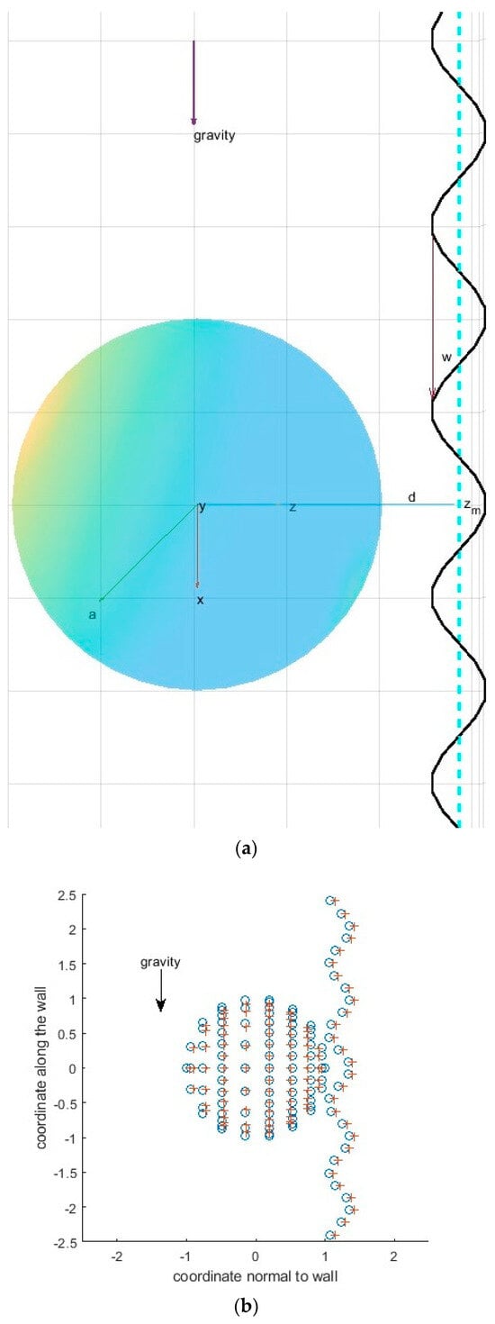
Figure 1.
Spherical particle moving under the action of gravity near a corrugated vertical wall: (a) domain set-up and (b) collocation points (o) and location of Stokeslets (+). Here, coordinate x is vertical along the action of the gravity force, coordinate z is directed normally to the wall, and coordinate y is perpendicular to the figure plane.
A viscous steady flow with Re < 1, which is caused by a moving particle under the action of gravity at the terminal state, is represented by the Stokes equations, which can be written as follows:
where (x,y,z) is the velocity vector field, p′(x,y,z) = p(x,y,z) − ρgx is the modified static pressure that accounts for the gravity term, and is the viscosity. The modified static pressure appears from the pressure and gravity forces in the original Stokes equations: ∂p/∂x − ρg = ∂(p − ρgx)/∂x. The stationary (fixed) particle is considered in Section 2 and Section 3, while the unsteady (moving) particle is considered in Section 4.
In experiments [3] using tweezers, a particle is placed nearby the corrugated surface and then released. Similar to Ref. [3], the flow field around the individual particle is tracked at the limit of low concentration of the particles. The viscosity of the fluid as opposed to the apparent macro-viscosity of a fluid with suspended particles, which will be dependent on the concentration of the particles, is assumed to be constant, as in analytical computations [3].
The boundary conditions are no-slip and no-penetrating at the wall and at the particle(s) surface. Therefore, the fluid velocity at the particle(s) surface is equal to the velocity of the particle.
The MFS involves two steps in its application: first, the substitution of the velocity, generated by the total NT Stokeslets with an unknown strength into the proper boundary conditions to construct a desired linear algebraic system of equations and the solution of this system; second, the use of the obtained strength of the Stokeslets to compute the velocity and pressure distributions for the entire domain. Three-dimensional velocity of the flow and the pressure induced by a point force (the Stokeslet) are given by [18]
and
where is the strength of an individual Stokeslet, is the distance between the location of the Stokeslet and the collocation point, and the superscripts and denote the components of the vectors and . The Einstein summation rule is used in the above equations.
The collocation points, in which the no-slip and no-penetration boundary conditions should be satisfied, are located at the surface of the particle and at the vertical wall (see Figure 1b). A uniform distribution of collocation points [10] is adopted in this study. This distribution assumes an approximately equal distance between collocation points over the spherical surface of the particle (Figure 1b).
To avoid a high condition number, c, of the linear systems to be solved, singularities (Stokeslets) are located outside of the computational domain, as shown in Figure 1b. The Stokeslets are submerged underneath the wall surface and the sphere surface. This way, the pole of the Green’s function moves away from the boundary onto a surface exterior to the flow [18,19,20,21]. The submergence of singularities for Stokes equations and the optimum depth of submergence were discussed in [10] and the references therein. The optimum depth of submergence is needed, because the condition number becomes large when the Stokeslets are moved excessively towards the sphere center. In Figure 2, the angle β, which is between the vectors directed from a collocation point to the locations of neighboring Stokeslets, tends to be zero when the Stokeslets are located farther away from the particle surface; therefore, the vectors directed from a collocation point to neighboring Stokeslets become nearly parallel to each other. As a result, the system matrix becomes ill-conditioned, because it contains nearly equal columns originating from the neighboring Stokeslets. A similar situation occurs when the number of Stokeslets and collocation points become large: the vectors directed from a collocation point to neighboring Stokeslets, which are located close to each other, become nearly parallel to each other. It should be mentioned here that the MFS suffers from an ill-conditioned matrix issue noticed by prior studies (see Ref. [22] and references therein). This linear algebra drawback can lead to inaccurate Stokeslets strengths and, consequently, inaccuracies in the induced flow field. It requires the selection of an optimal number of collocation points and Stokeslets that will be addressed in the next section.
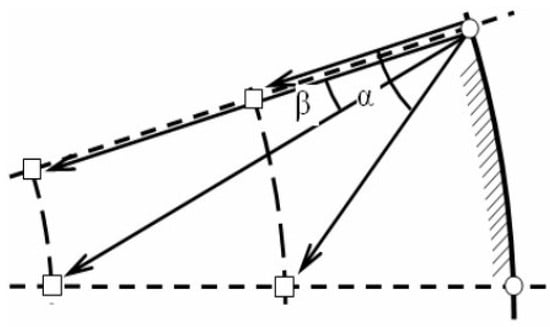
Figure 2.
Submergence of Stokeslets: vectors directed from a collocation point to two neighboring Stokeslets. Here, squared and circular symbols refer to the Stokeslets and collocation point positions, respectively, and α and β are the angles between vectors, where the angle β corresponds to a larger distance between collocation points and locations of Stokeslets.
As another way to improve the accuracy of the MFS and reduce the condition number, we can use the Stokeslets’ regularization technique presented in [23,24]. This technique was introduced to avoid singularity at the boundaries. The accuracy of the MFS with submerged and/or regularized singularities depends on the placement of singularities and on the value of the regularization parameter. The regularization is introduced using a so-called blob function with its regularization parameter, ε [23,24], replacing the Dirac delta function for Stokeslets, which shows the singularity at the center of the Stokeslet. The spatially smoothed approximation by the blob function to the singular 3D Dirac delta function is plot in [24] for a few representative values of ε. The authors [23] showed theoretically (see [23], Equation (21)) the order of discretization errors as a function of the regularization parameter, ε. Also, they presented the error obtained by numerical computations as a function of this parameter. The value of ε = Δs/4, where Δs is the distance between Stokeslets, was introduced first in Ref. [24], Section 3.1, by numerical experimentation. The authors (see [24], Section 3.2) stated that the MFS solution is not very sensitive to the coefficient of proportionality between ε and Δs as soon as the coefficient is smaller than one. By more extensive analysis [23], the value of ε = Δs/4 corresponds to the area of the minimum of the discretization error (see [23], Figure 2), and therefore, this value is selected in the present study.
The equations for the velocity for the Stokeslets with the regularized singularities are as follows:
where .
As will be shown in the next section, the most accurate MFS results are obtained by a combination of the submergence of Stokeslets and their regularization.
The above system (3) or its regularized version (5) can be expressed in the matrix form for an arbitrary 3D Stokes flow as follows:
where is a velocity vector at the collocation points (boundary conditions), is a Stokes force vector with 3NT unknowns, and M is the 3NT × 3NT matrix of the above system. The Stokes force vector has the structure of. Since the pressure is modified (see explanation after Equation (2)) the normal force exerted on the particle includes the buoyance force exerted by the fluid. For the past implementation of the MFS [10,13] for the flow field determined by far field velocity, the velocity vector at the collocation points is set up as equal to zero for no-slip and no-penetrating boundary conditions, while the known non-zero constant velocity is selected at the far field. In the current study, the velocity vector, includes the unknown velocities at the particle surface, ux, uy, and uz. As soon as the particle is non-deformable and non-rotating, its velocity components, ux, uy, and uz, are the same for all collocation points. It is assumed that the particle has reached its terminal velocity.
Ref. [25] and the references therein compared the Stokes force calculated by Faxen, who solved Oseen’s equation allowing the sphere to rotate, and by O’Neill, who solved the Stokes equation using bipolar coordinates without rotation. In Ref. [25], in Figure 1, the authors concluded that the obtained Stokes force for non-rotating computations by O’Neill and rotating computations by Faxen were close to each other and close to the experimental results [25] as soon as the parameter determining the proximity of the particle to the wall, e, was between 0.04 and 0.4. In the present study, the value of e is within this range (see Section 3). Therefore, the rotation of particles is neglected in the present study and will be considered in future research.
Note that, if the rotational velocity needs to be accounted for, the no-slip boundary conditions at the particle surface are extended, u = Ω ∧ r, where u = (ux, uy, uz), Ω is the instantaneous rotational velocity of the sphere, and r is the radius vector from the center of the sphere to the sphere surface. The torque, MΩ, needs to be calculated to obtain Ω [17].
Because of the presence of the three new unknowns, ux, uy, and uz, in the vector , the system (6) requires the addition of three equations representing the terminal (sedimentation) state of the particle motion with no acceleration:
where N is the number of Stokeslets per particle, and W is the weight force directed in the x direction and equal to one in the normalized variables.
The above equations represent the condition that the resultant force is equal to the sum of Stokeslets at the terminal state of the particle motion, where the gravity force is directed along coordinate x. After the addition of three equations (7) and three unknown velocities to the system (6), its size becomes (3NT + 3) × (3NT + 3). The numerical solution of the above linear system (6) is performed using the MATLAB backslash linear algebraic operation, F = U\M [26].
Once the above linear system is solved, the velocity at any point of the flow field can be calculated by substituting the Stokeslets, which are obtained by solving (6), either into (3) or into its regularized version, (5).
3. Computational Parameters of the MFS and Comparison of the Numerical Results with an Approximate Analytical Solution
In this section, the particle is located at a fixed location with respect to corrugation (Figure 1a). The corrugations are horizontal, and the number of corrugations is unlimited. The MFS solution is compared to the prior approximate analytical solution of the flow field around the sedimented particle near the corrugated wall [1,3,17]. The set of MFS computational parameters is selected to ensure numerical accuracy and computational efficiency.
The geometric parameters listed below are normalized by the radius of the particle. The center of particle is located at the origin. The given amplitude of corrugation, zm, is equal to 0.15, and the corrugation wavelength, w, is equal to one. The distance between the sphere and the corrugation-free wall in the z direction, d, is equal to 0.2, so the minimum distance between the particle’s surface and the wall is 0.05, and the distance between the wall and the center of the particle is 1.2. The ratio of distance to the wall to the particle radius is e = 0.2/1 = 0.2. The location of the center of particle with respect to a neutral level of corrugation is determined by the parameter :
For φ at its limit values, 0 or 1, the particle is facing the corrugated wall corresponding to the zero value of the sinus; that is, the distance from particle to wall is z = d. The values of φ = 0.25 and φ = 0.75 correspond to the maximum, and minimum, distance between particle and wall; that is, the maximum and minimum of the sin function in Equation (8). At the mid-values of the phase parameter, φ~0.5, the particle is facing a neutral level of corrugation; however, the gravity force is acting toward the corrugation in this case, whereas, for φ at 0 or 1, the gravity force is acting toward the fluid. For the MFS computations presented in Figure 3 and Figure 4, the interval 0 ≤ φ ≤ 1 is divided into 36 equal cells, from 0 or 1, and the MFS system of Equations (2)–(7) is solved for each value of φ. The corrugations are non-tilted (horizontal) with respect to gravity, and therefore, they do not create a velocity component in the y direction.
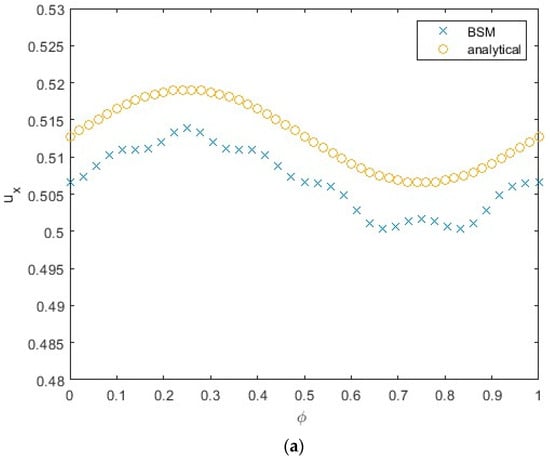
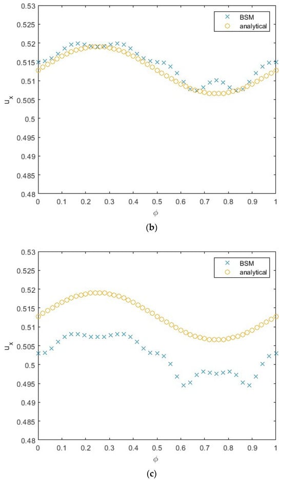
Figure 3.
Velocity component ux parallel to the un-corrugated wall (along gravity) as a function of the parameter φ (phase of sin-type corrugation, see Equation (8)), and analytical solution (Ref. [3], p. 7) of the Stokes equations near the corrugated wall. The number of Stokeslets and number of collocation points per spherical particle: (a) N = 100, (b) N = 150, and (c) N = 200.
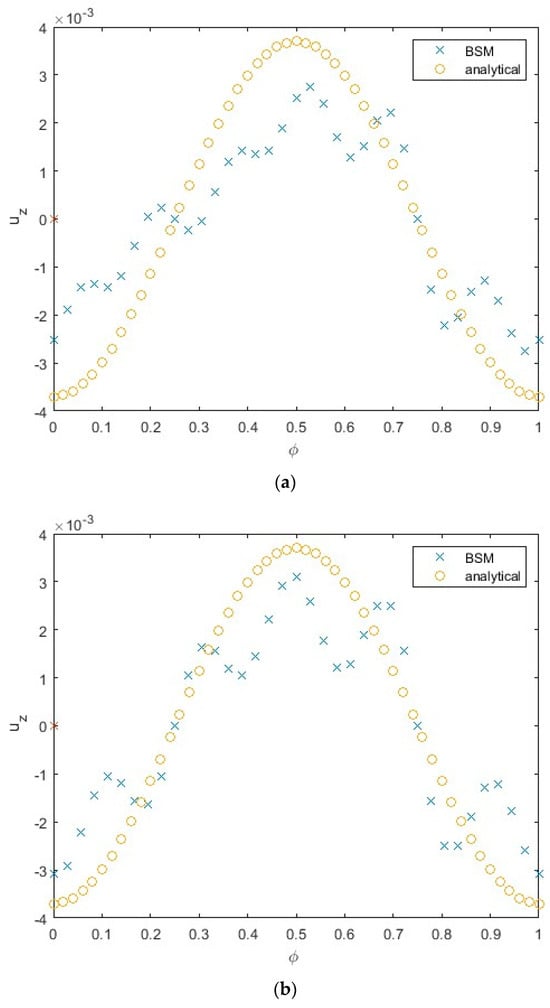
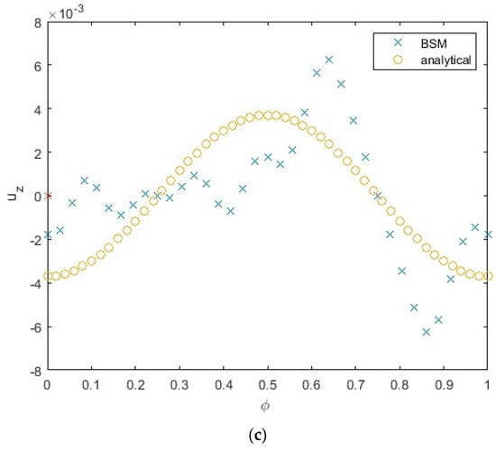
Figure 4.
Velocity normal to the wall for (a) N = 100, (b) N = 150, and (c) N = 200 as a function of the parameter φ. Velocity obtained by the MFS is compared to the analytical solution (Ref. [3], p. 7).
The most accurate MFS results are obtained by regularized submerged Stokeslets for a submergence depth for the Stokeslets of 0.05 for the spherical particle and 0.075 for the wall. The approximate distance between collocation points on the sphere is
where a is the radius of the sphere, and N is the number of submerged Stokeslets and the number of collocation points on the sphere surface. The locations of the Stokeslets and collocation points are steady with respect to the center of the particle.
The Stokeslets located along the wall are placed half the distance between the neighboring Stokeslets in the x and z directions, , where Δ is defined by Equation (9). The MFS solution with N = 150 for the velocity component parallel to the wall coincides fairly with the analytical solution [1,3] of the Stokes equations near the corrugated wall (Figure 3b). The results in terms of vertical velocity for N = 100 (Figure 3a) deviate from the analytical solution by 2%, whereas the results for N = 200 (Figure 3c) deviate from the analytical solution by 2.4%. The larger deviation from the analytical solution is explained by the insufficient number of Stokeslets for N = 100 and the large condition number of the matrix, M, for N = 200 (see the discussion below). In Table 1, the MFS results are also presented for a smooth vertical wall located at the same distance from the particle for comparison to the ux results (Figure 3). The velocity for a smooth vertical wall in Table 1 can be compared to that obtained by O’Neill, who solved the Stokes equation using bipolar coordinates without rotation [25]. For this purpose, the velocity is obtained from the expression for the normalized vertical Stokes force depicted in Figure 1, Ref. [25]. The obtained value of the velocity for a particle near the smooth wall is ~0.5, which corresponds fairly well to the MFS results presented in the rightmost column in Table 1.

Table 1.
The elapsed computational time of the presented numerical simulations.
The velocity component normal to the wall differs from the analytical solution of the Stokes equations developed in Refs. [1,3] for some values of φ (Figure 4), especially those corresponding to the particle facing the depth of the sin profile of roughness—that is, for mid-values of the phase parameter. The magnitude of the normal component of the velocity is O(10−3) (Figure 4), while the magnitude of the component of the velocity parallel to the wall is O(1) (Figure 3); therefore, the relative error of the velocity normal to the wall, uz, is larger than that for the velocity in the direction of gravity, ux, while the absolute error is larger for the component ux.
The results obtained by using a 10 × 10 x-y domain are very close to those obtained by a 15 × 15 domain, therefore, the results in Figure 4 are presented for a 10 × 10 domain. In Figure 4, the MFS results are presented for the following numbers of Stokeslets per sphere: N = 100 (Figure 4a), N = 150 (Figure 4b), and N = 200 (Figure 4c). The results for N = 150 are closer to the analytical solution compared to those for N = 100 (compare Figure 4a to Figure 4b). The results for N = 200 show the deviation from the analytic values with the increase in magnitude of the velocity, uz, for some values of φ. This can be explained by the dramatic increase in the condition number, c ~ 107, for N = 200. This value of the condition number is much larger than that for N = 100 (c ~ 650) and for N = 150 (c ~ 2300).
The convergence study with respect to the number of Stokeslets, N, should be conducted until the increase in condition number by an order of magnitude that negatively affects the accuracy of the MFS.
In Table 1, the computational cost (in terms of elapsed computational time) for a single value of the parameter φ is presented for the range of numbers of Stokeslets at the sphere: N = 100, 150, and 200. The computer used is a PC OptiPlex 9020 manufactured by Dell, Round Rock, Texas USA, with a processor Intel(R) Core(TM) i7-4790 CPU @ 3.60 GHz, with 4 Cores. MATLAB reads the internal time at the execution of the toc function and displays the elapsed time since the most recent call to the tic function without an output. The elapsed time is expressed in seconds.
The computational time includes the solution of the linear algebraic system (6), F = U\M, using MATLAB’s linear algebraic backslash operation. The total elapsed time includes the solution of the linear system by Equations (6) and (7) and the setting up of matrix M by Equations (2.3) and (2.5). The computational cost of the solution of the linear MFS system is O(Nγ), where the exponent γ satisfies 2 < γ < 3. The construction of matrix M before the solution of the linear MFS system is O(N2), where N2 is the number of elements of M. By computing a linear regression of the logarithm of the computer time for the backslash operation with log N (see Table 1), we obtain the slope of regression line γ = 2.9.
The fraction of the total computer time to compute the matrix M drops from 24.6% for N = 100 to 15.8% for N = 200. Assuming the total computer time ~O(Nδ), by a linear regression of the logarithm of the total computer time with log N (see Table 1), we obtain δ = 2.74.
As shown above in this section, the MFS suffers from an ill-conditioned matrix issue associated with finding the Stokeslets’ strengths, which can lead to inaccurate Stokeslet strengths and, consequently, inaccuracies in the computed flow field (see Ref. [22] and references therein). The authors [22] used Tikhonov regularization to solve ill-conditioned linear systems of equations. Their algorithm is based on introducing a regularization parameter into the original MFS matrix. This approach could be tested in future research.
Recently, a localized MFS (LMFS) was developed (see [27] and references therein). The LMFS combines the concept of localization and the MFS. The resultant system of linear algebraic equations in the LMFS is sparse and banded and, thus, could reduce the condition number, storage, and computational burden of the MFS. The LMFS will be verified and adopted for the considered set-up in future research.
4. MFS Computations for a Particle Moving near the Corrugations Tilted with Respect to Gravity
In this section, the results of the MFS computations are presented to determine the trajectory of the particle near the corrugated wall with tilted corrugations with respect to gravity. The computational parameters are the same as those obtained in previous sections, unless otherwise stated. The N = 150 Stokeslets per spherical particle will be used in this section, as this number of Stokeslets corresponds to the most accurate solution for the ux (Figure 3) and uz (Figure 4) velocity components in the past section. While the locations of Stokeslets and collocation points at the particle are steady with respect to the center of the particle, their locations move with the moving particle.
The author compared the theoretical and experimental results (see Figure 3 in Ref. [3]) against the MFS computations. The derivation of the approximate analytical solution of the Stokes equations for prediction of the roughness-induced velocity is presented in Ref. [3], p. 7. The experimental methodology of imaging of the trajectory of the particle involved in sedimentation near a 3D-printed corrugated surface is presented in Ref. [3], p. 6. In these experiments using tweezers, a particle is placed nearby the corrugated surface and then released. To minimize the effect of the initial release/unsteadiness, the particle is allowed to sediment ~10 times its radius before recording its trajectory [3]. The two 3D-printed corrugations of sinusoidal shape, Equation (1), are tilted at an angle of 45 degrees to the vertical gravity force. The tilted corrugation wavelength λ = 6 mm. The particle’s radius is 1.6 mm, and the initial distance between the particle surface and the smooth wall is 0.2 mm.
The length of the domain along the vertical coordinate, x, is L = 3.5λ, centered at x = 0. A particle starts at 0.75λ upstream of the first corrugation, and the trajectory ends at 0.75λ downstream of the second corrugation. Initially, the particle distance to the wall is equal to 0.2 mm, as specified above. The size of the wall surface domain where the collocation points are located—that is, in the y and x directions—is 10a × 10a, where a is the particle radius. The computational domain is centered at the current particle location and moves together with the moving particle after each time step. Varying the domain size from 8a × 8a to 15a × 15a does not affect the obtained particle trajectory. Note that there is no need to define the domain in the z direction, within the fluid domain, as the Stokeslets and collocation points are not located in the z direction. A total of 200 equal time steps of length Δt is taken to follow the particle’s motion along the vertical x coordinate over two corrugations.
At each time step, the flow field around the particle is assumed to become relaxed to the steady-state Stokes Equation (2). The new values of velocity, ux, uy, and uz, are found by the solution of the linear system (6). After computing the new velocity, the new coordinates of the particle are found by the following relations:
where are the new coordinates of the particle after the time step Δt, are the old coordinates of the particle, and Δt is the time step.
For each time step, the linear system (6) representing the MFS must be formed and solved [28].
The results presented in Figure 5 compare MFS computations against published experimental and analytical results (see Figure 3B [3]). From Figure 5, the distance in the normal direction from the smooth wall is normalized by the corrugation wavelength, z/λ, and presented as a function of the vertical coordinate along the wall, x/λ. As depicted in Figure 5, the results of the MFS computations are located closer to the experimental data points compared to the results obtained by the analytical method in areas near the minimum of z/λ. For areas near the maximum of z/λ, the analytical and MFS computations are closer to each other compared to the areas of the minimum. From Figure 5, the amplitude of the sin-type oscillations, z/λ, computed by the MFS is smaller than that computed by the analytical method.
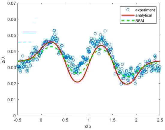
Figure 5.
Comparison of the distance to the wall obtained by the MFS to the published analytical and experimental results [3] for particle moving by the action of gravity along tilted corrugations, where x/λ is the normalized distance along the wall and z/λ is the normalized distance normal to the wall.
The results in Figure 6 compare the lateral displacements obtained by the MFS computations against the published experimental and analytical results (see Figure 3C [3] for sinusoidal corrugation). In Figure 6, the lateral horizontal displacement along the wall, y, is normalized by the corrugation wavelength, y/λ, and presented as a function of the normalized coordinate along the wall, x/λ. The results in Figure 6 show that the obtained MFS maxima of the magnitude of the lateral displacement, in terms of y/λ, are not as prominent as the maxima obtained analytically and experimentally [3], but they still coincide in terms of their locations, x/λ, and distance between the maxima. The correspondence of the locations of the extrema for the analytical and MFS solutions in Figure 5 and Figure 6 is explained by the fact that the difference between the analytical and computed values of the vertical velocity, ux, is within 1% for N = 150 (Figure 3b).
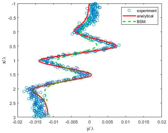
Figure 6.
Comparison of the normalized lateral displacement of the particle, y/λ, obtained by the MFS to the published analytical and experimental results [3].
5. MFS Modeling of the Motion of Two Particles near the Corrugated Wall
The discussion in this section aims at monitoring the difference between the motion of a single particle discussed in the previous section and the tandem of particles and investigating the role of the computational parameters, such as the number of Stokeslets per spherical particle.
Each of the two particles is assumed to be non-deformable and non-rotating; therefore, their velocity components, ux, uy, and uz, are the same for all collocation points belonging to the same particle. The rotation of the particles will be considered in the future research, as outlined in Section 2. It is assumed that each particle has reached its individual terminal velocity. The presence of six new unknowns, ux,1, uy,1, uz,1, and ux,2, uy,2, and uz,2, in the vector requires the addition of six equations to the system (6). These equations represent the condition for the resultant force to become equal to zero at the terminal state of each particle motion (see the similar Equation (7) for a single particle). The sum of the Stokeslets strengths in the y and z directions is therefore equal to zero. The particle’s weight is equal to the sum of the Stokeslets in the x direction.
The set-up of two particles near the corrugated wall and the distribution of static pressure computed by Equation (4) with the modification for regularized Stokeslets [24] is shown in Figure 7. Initially, the particles were in the same proximity to the vertical wall. The initial distance between the centers of the particles in the vertical direction, x, is equal to 5a, where a is the radius of the particle. The first particle is initially located at 0.75λ up the first corrugation (the same location as the single particle in the previous section). The second particle is located at 5a up the first particle. Initially, the particles’ distance to the wall in the z direction is equal to 0.2 mm, as specified in Section 4. When particles move, each of them appears at a different distance z from the wall, as shown in Figure 8a.
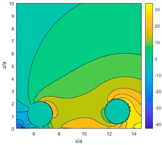
Figure 7.
Set-up of two particles located near the corrugated wall with a computed distribution of the static pressure. The coordinate x is centered at the mid-point between particles and extends 5a upstream and downstream.
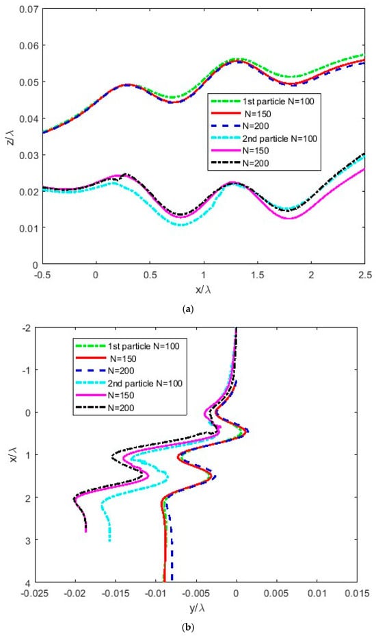
Figure 8.
Trajectories of two particles undergoing sedimentation along a rough wall, x/λ, computed by the MFS: (a) deviation from the vertical trajectory in terms of the normal direction to the wall, z/λ, and (b) deviation in the horizontal direction along the wall, y/λ. The MFS computations are presented for the number of Stokeslets per spherical particle: N = 100, 150, and 200. Particles move along the x axis from left to right in (a) and up–down in (b).
In Figure 8, the trajectories of the two particles moving along the corrugated wall under the action of gravity are depicted. To obtain the trajectories, MFS computations for 200 time steps are conducted for the number of Stokeslets per spherical particle: N = 100, 150, and 200. In Figure 8a, the deviation from the vertical trajectory in terms of the normal direction to the wall, z/λ, is shown. Recall that the initial value of z/λ = 0.2 mm/6 mm = 0.033 for both particles. In Figure 8b, the deviation in the horizontal direction along the wall, y/λ, is depicted.
In Figure 8a, the first (located down the wall) particle is pushed away from the wall by the moving second (located up the wall) particle in its wake, whereas the second particle is moving in closer proximity to the wall compared to its initial distance from the wall. In Figure 8b, the first particle follows a path that is qualitatively like that of a single particle in Figure 6. However, its deviation from the vertical trajectory, y/λ, is less prominent compared to that for a single particle (Figure 6), as its distance from the surface roughness is larger. On the contrary, the deviation of the second particle in the y direction is more than doubled compared to that of a single particle (Figure 6), as the second particle passes closer to the wall roughness.
The vertical, z/λ, displacements are qualitatively similar for a varying number of Stokeslets, from N = 100 to N = 200, as shown in Figure 8a. As shown in Figure 8a, the trajectories converge when the number of Stokeslets per spherical particle increases from N = 100 to N = 200 because of the cancellation of the MFS errors in the computed velocity when the velocity is integrated in time by Equation (10). The horizontal, y/λ, displacement for the second particle shows some oscillations (see Figure 8b). For the smallest number of Stokeslets, N = 100, the deviation of the second particle from the vertical direction is less prominent compared to that for the larger number of Stokeslets, N = 150 and 200.
6. Conclusions
The Method of Fundamental Solutions (MFS) is developed and applied to a particle(s) moving along a corrugated wall under the action of gravity to obtain the particles’ local velocity and trajectory. The MFS linear system is modified to compute the unknown particles’ velocity and account for the gravity force as a driver for the particles’ motion. The combination of regularization and submergence of Stokeslets is implemented to maintain a moderate value of the condition number of the MFS matrix to ensure the accuracy of the solved linear system for the challenging case of closed proximity between the particle and the wall. The obtained trajectory of a particle, including its lateral displacement, does correspond to published experimental data and approximate analytical solutions of the Stokes equations.
Using the obtained set of MFS parameters, the method is extended to the case of two moving particles in proximity to the corrugated wall in a case where an analytical solution for the Stokes equations is not available. The results show that the particles deviate from the trajectory of a single particle, where the forward (down) particle moves farther away from vertical wall in the z direction and the back (up) particle shifts closer to the wall. As a result, the horizontal deviation along the wall of the forward particle, y, is smaller, whereas the horizontal deviation of the back particle is larger compared to that for a single particle.
In future research, the MFS will be extended to more complex situations of sedimentation in which an analytical solution is not available, such as stochastic non-periodical wall roughness and clusters of particles shaped as either multiple spheres or Cassini ovals.
Funding
The author would like to thank the Visitors Program of Max Planck Institute for the Physics of Complex Systems (MPI) in Dresden, Germany, where this study started, to enable his research visit in Fall 2022 during his sabbatical leave from the University of Akron.
Data Availability Statement
The original contributions presented in the study are included in the article, further inquiries can be directed to the corresponding author.
Acknowledgments
The author acknowledges Christina Kurzthaler, Research Group Leader, MPI, for the discussion and for pointing the author to her published analytical results for the Stokes equations for comparison to the presented MFS computations. MATLAB version R2022b is used in the current study.
Conflicts of Interest
The author declares no conflicts of interest.
List of Symbols
| a | Radius of spherical particle |
| c | Condition number of matrix M |
| d | Distance between the sphere and the smooth wall |
| Strength of Stokeslet | |
| M | Matrix of MFS system |
| N | Number of Stokeslets and collocation points per spherical particle |
| p | Static pressure in the flow field |
| p′ = p − ρgx | Modified static pressure that accounts for gravity term |
| Distance between the location of the Stokeslet and the collocation point | |
| Velocity vector at collocation points | |
| Fluid velocity vector | |
| ux, uy and uz | Particle velocity components |
| W | Weight force exerted on particle in the x direction |
| w | Wavelength of periodical wall roughness |
| x | Up–down coordinate along the wall |
| Coordinates of particle at the end of time interval | |
| Coordinates of particle at the beginning of time interval | |
| y | Horizontal coordinate along the wall |
| z | Normal direction to the wall |
| zm | Magnitude of the wall roughness. |
| β | Power in the estimate of the computational cost of the solution of the linear MFS system, O(Nβ) |
| λ | Tilted corrugation wavelength |
| δ | Power in the estimate of the total elapsed computer time, O(Nδ) |
| Distance between collocation points at sphere surface | |
| Δs | Distance between Stokeslets |
| Δt | Time step to compute the new location of a particle |
| ε | Value of the regularization parameter |
| Viscosity | |
| Phase parameter of wavelength corrugation | |
| and | Superscripts that denote components of the vectors and |
References
- Kurzthaler, C.; Stone, H.A. Microswimmers near corrugated, periodic surfaces. Soft Matter 2021, 17, 3322. [Google Scholar] [CrossRef] [PubMed]
- Lauga, E.; Powers, T.R. The hydrodynamics of swimming microorganisms. Rep. Prog. Phys. 2009, 72, 096601. [Google Scholar] [CrossRef]
- Chase, D.L.; Kurzthaler, C.; Stone, H.A. Hydrodynamically Induced Helical Particle Drift due to Patterned Surfaces. Proc. Natl. Acad. Sci. USA 2022, 119, e2202082119. [Google Scholar] [CrossRef] [PubMed]
- Yao, Z.; Wang, H. Some benchmark problems and basic ideas on the accuracy of boundary element analysis. Eng. Anal. Bound. Elem. 2013, 37, 1674–1692. [Google Scholar] [CrossRef]
- Mukherjee, S.; Liu, Y. The Boundary element method. Int. J. Comput. Methods 2013, 10, 1350037. [Google Scholar] [CrossRef]
- Liu, Y. Fast Multipole Boundary Element Method; Cambridge University Press: Cambridge, MA, USA, 2010. [Google Scholar]
- Fairweather, G.; Karageorghis, A. The method of fundamental solutions for elliptic boundary value problems. Adv. Comput. Math. 1998, 9, 69–95. [Google Scholar] [CrossRef]
- Askour, O.; Tri, A.; Braikat, B.; Zahrouni, H.; Potier-Ferry, M. Method of fundamental solutions and high order algorithm to solve nonlinear elastic problems. Eng. Anal. Bound. Elem. 2018, 89, 25–35. [Google Scholar] [CrossRef]
- Cheng, A.; Hong, Y. An overview of the method of fundamental solutions—Solvability, uniqueness, convergence, and stability. Eng. Anal. Bound. Elem. 2020, 120, 118–152. [Google Scholar] [CrossRef]
- Mikhaylenko, M.; Povitsky, A. Optimal Allocation of Boundary Singularities for Stokes Flows about Pairs of Particles. Eng. Anal. Bound. Elem. (EABE) 2014, 41, 122–138. [Google Scholar] [CrossRef]
- Zhao, S.; Povitsky, A. Three-dimensional boundary singularity method for partial slip flows. Eng. Anal. Bound. Elem. 2011, 35, 114–122. [Google Scholar] [CrossRef]
- Zhao, S.; Povitsky, A. Boundary Singularity Method for Partial Slip Flows. Int. J. Numer. Methods Fluids 2009, 61, 255–274. [Google Scholar] [CrossRef]
- Mikhaylenko, M.; Povitsky, A. Combined boundary singularity method and finite volume method with application to viscous deformation of polymer film in synthesis of sub-micron fibers. Eng. Anal. Bound. Elem. 2017, 83, 265–274. [Google Scholar] [CrossRef]
- Topuz, A.; Baranoğlu, B.; Çetin, B. A multi-domain direct boundary element formulation for particulate flow in microchannels. Eng. Anal. Bound. Elem. 2021, 132, 221–230. [Google Scholar] [CrossRef]
- Sun, Q.; Klaseboer, E.; Khoo, B.C.; Chan, D.Y. Boundary regularized integral equation formulation of Stokes flow. Phys. Fluids 2015, 27, 023102. [Google Scholar] [CrossRef]
- Aboelkassem, Y.; Staples, A.E. Stokeslets-meshfree computations and theory for flow in a collapsible microchannel. Theor. Comput. Fluid Dyn. 2013, 27, 681–700. [Google Scholar] [CrossRef]
- Kurzthaler, C.; Zhu, L.; Pahlavan, A.A.; Stone, H.A. Particle motion nearby rough surfaces. Phys Rev. Fluids 2020, 5, 082101. [Google Scholar] [CrossRef]
- Pozrikidis, C. Boundary Integral and Singularity Methods for Linearized Viscous Flow; Cambridge University Press: Cambridge, MA, USA, 1992. [Google Scholar]
- Gonzalez, O. On stable, complete and singularity-free boundary integral formulations of exterior Stokes flow. Soc. Ind. Appl. Math. (SIAM) J. Appl. Math. 2009, 69, 933–958. [Google Scholar] [CrossRef]
- Hebeker, F.K. A boundary element method for Stokes equations in 3-D exterior domains. In The Mathematics of Finite Elements and Applications; Whiteman, J.R., Ed.; Academic Press: London, UK, 1985; pp. 257–263. [Google Scholar]
- Koens, L.; Lauga, E. The boundary integral formulation of Stokes flows includes slender-body theory. J. Fluid Mech. 2018, 850, R1. [Google Scholar] [CrossRef]
- Aboelkassem, Y.; Staples, A.E. A three-dimensional model for flow pumping in a microchannel inspired by insect respiration. Acta Mech. 2014, 225, 493–507. [Google Scholar] [CrossRef]
- Cortez, R.; Fauci, L.; Medovikov, A. The method of regularized Stokeslets in three dimensions: Analysis, validation, and application to helical swimming. Phys. Fluids 2005, 17, 031504. [Google Scholar] [CrossRef]
- Cortez, R. The method of regularized Stokeslets. SIAM J. Sci. Comput. 2001, 23, 1204–1225. [Google Scholar] [CrossRef]
- Ambari, A.; Manuel, B.G.; Guyon, E. Effect of a plane wall on a sphere moving parallel to it. J. Phys. Lett. 1983, 44, 143–146. [Google Scholar] [CrossRef]
- Chapra, S.C. Applied Numerical Methods with MATLAB, 3rd ed.; McGraw Hill: New York, NY, USA, 2012; p. 588. [Google Scholar]
- Qu, W.; Fan, C.-M.; Li, X. Analysis of an augmented moving least squares approximation and the associated localized method of fundamental solutions. Comput. Math. Appl. 2020, 80, 13–30. [Google Scholar] [CrossRef]
- Mitchell, W.H.; Spagnolie, S.E. Sedimentation of spheroidal bodies near walls in viscous fluids: Glancing, reversing, tumbling, and sliding. J. Fluid Mech. 2015, 772, 600–629. [Google Scholar] [CrossRef]
Disclaimer/Publisher’s Note: The statements, opinions and data contained in all publications are solely those of the individual author(s) and contributor(s) and not of MDPI and/or the editor(s). MDPI and/or the editor(s) disclaim responsibility for any injury to people or property resulting from any ideas, methods, instructions or products referred to in the content. |
© 2024 by the author. Licensee MDPI, Basel, Switzerland. This article is an open access article distributed under the terms and conditions of the Creative Commons Attribution (CC BY) license (https://creativecommons.org/licenses/by/4.0/).