Accuracy of Holographic Real-Time Mode Decomposition Methods Used for Multimode Fiber Laser Emission

Abstract

Mode decomposition is a powerful tool for analyzing the modal content of optical multimode radiation. There are several basic principles on which this tool can be implemented, including near-field intensity analysis, machine learning, and spatial correlation filtering (SCF). The latter is meant to be applied to a spatial light modulator and allows one to obtain information on the mode amplitudes and phases of temporally stable beams by only analyzing experimental data. As a matter of fact, techniques based on SCF have already been successfully used in several studies, e.g., for investigating the Kerr beam self-cleaning effect and determining the modal content of Raman fiber lasers. Still, such techniques have a major drawback, i.e., they require acquisition times as long as several minutes, thus being unfit for the investigation of fast mode distribution dynamics. In this paper, we numerically study three types of digital holograms, which permits us to determine, at the same time, the parameters of a set of modes of multimode beams. Because all modes are simultaneously characterized, the processing speed of these real-time mode decomposition methods in experimental realizations will be limited only by the acquisition rate of imaging devices, e.g., state-of-the-art CCD camera performance may provide decomposing rates above 1 kHz. Here, we compare the accuracy of conjugate symmetric extension (CSE), double-phase holograms (DPH), and phase correlation filtering (PCF) methods in retrieving the mode amplitudes of optical beams composed of either three, six, or ten modes. In order to provide a statistical analysis of the outcomes of these three methods, we propose a novel algorithm for the effective enumeration of mode parameters, which covers all possible beam modal compositions. Our results show that the best accuracy is achieved when the amplitude-phase mode distribution associated with multiple frequency PCF techniques is encoded by Jacobi–Anger expansion.

1. Introduction

Recently, the optics and photonics community has been witnessing a renewed interest in multimode (MM) optical platforms [1]. This has pushed researchers to take a broader look at systems like telecommunication links and mode-locked and Raman fiber lasers (RFL), for which single-mode fibers have been historically preferred. In particular, MM RFLs have attracted a great deal of interest owing to their extreme flexibility in terms of operating wavelengths [2] and to the high efficiency in the conversion of multimode pump light into high-quality Stokes emission. As a matter of fact, recent studies have reported on the effect of brightness enhancement of the Stokes beam in graded-index (GRIN) MM RFLs [3,4]. Generally speaking, a proper investigation of the dynamics of optical beams in MM platforms has required the development of novel measurement techniques, like those of mode decomposition (MD). MD methods can be based on several approaches, like genetic algorithms [5], phase modulation via spatial light modulators (SLM) [6], and deep learning [7,8]. Remarkably, when applied to few-mode beams, the decomposing rate of the latter may be as high as a few hundred Hz, the speed-limiting factors being the camera performance and the computing resources. On the other hand, the SLM-based technique, which is known as the spatial correlation filtering (SCF) method, may require a much longer measurement time, during which the beam has to be stable. Still, SCF has a great advantage, i.e., its applicability is not limited by the number of modes. For this reason, SCF turned out to be extremely powerful in fundamental science. For instance, phase-only SLM devices were used for the MD of MM RFL beams, as well as for investigating the so-called Kerr beam self-cleaning effect [9,10,11], and validating its description in the framework of optical thermodynamics [12].

In spite of these successful examples, there is still room for improving MD methods in terms of speed, accuracy, and flexibility, e.g., using special mode bases. For instance, as it was used in [11], the SCF method requires an acquisition time as long as several minutes, thus being unfit for the investigation of real-time mode distribution dynamics. As a matter of fact, real-time MD remains an urgent task, especially in the context of the investigation of transverse mode instability phenomena in high-power fiber lasers and amplifiers [13,14,15,16,17]. In these cases, in fact, the correct interpretation of the mode distribution can only be achieved in an experimental way. In this regard, possible ways of MD multiplexing were proposed by different research groups. The general idea is to create a diffraction element that is able to split correlation signals for different modes in space; in this way, the amplitude and phase of more than one mode can be measured simultaneously. For example, it was shown that one can resolve eight modes at once by using specifically manufactured amplitude-phase mode analyzing elements [18]. Since most SLMs are phase-only devices, the SCF method cannot be applied directly. However, it is well-known that by grouping pixels of SLM and forming so-called double-phase holograms (DPH), one can imitate amplitude modulation even with phase-only devices [19]. In this regard, it has to be mentioned that a method developed directly for phase-only SLM was reported by Zhao et al. in 2019 [20]. This is based on the encoding of a mode array into a hologram using a conjugate symmetric extension (CSE) method. In addition, the original SCF technique can also be multiplexed, as described in [18]. Such a multiplexing method was successfully applied, for the first time, by Flamm et al. in 2012 to a beam composed of three modes [6]. It should be noted that all aforementioned methods do not require larger computational resources and are limited only by the camera performance, so that, in principle, the decomposing rate can exceed 1 kHz for modern high-speed devices, regardless of the multiplexed mode number. But the more modes one would like to measure in parallel, the more complex a hologram should be encoded. To the best of our knowledge, limitations on the number of modes depending on the type of hologram have never been investigated.

In this work, we used numerical models to compare the above methods in terms of the accuracy of modal amplitude retrieval in a set of well-defined multimode beams. In order to make a representative sample of beams with a variety of modal content, a special algorithm of amplitude combination enumeration was developed. Compared to the case of a randomly generated set of amplitudes, which is used, for example, to prepare datasets in machine learning methods, our algorithm allows us to compare the accuracy of different MD methods in absolutely identical initial conditions and covers the space of all possible amplitude combinations uniformly. In particular, we considered the cases of three, six, and ten modes multiplexed in one hologram, allowing real-time measurements. These cases correspond to the previous investigations based on deep learning techniques [7,8] and to the number of modes for the firsts three principal quantum numbers for a GRIN fiber (namely, PQN $=1,2,3$). Our results indicate that, among the SCF-based routines we tested, the most effective in terms of MD accuracy is the one based on a phase spatial correlation filter with the use of the Jacobi–Anger expansion.

2. Algorithm of Mode Combination Enumeration

First of all, we present an algorithm that allows us to obtain a reproducible set of mode amplitudes and cover the space of all possible combinations uniformly. Let us dub $v_m$ the intensity of the p-th mode with $m=1,\dots ,M$, being M the number of modes. Now, let us consider that each mode intensity may assume a value that belongs to a discrete set of values (levels of intensity). For the sake of simplicity, let us consider the following n levels of intensity $\{i_1,i_2,\dots ,i_n\}$:

$$i_p=\frac{1}{n-1}(p-1),p=1\dots n,$$

(1)

Finally, let us neglect the phase associated with each mode, i.e., we suppose that all the modes have the same phase equal to zero. We make this assumption for several reasons: Not all methods considered here are able to retrieve phases, and to retrieve the phases it is necessary to retrieve the amplitudes first. To calculate inaccuracies we use the dot product between the initial and retrieved amplitude vectors, so that the phases do not contribute to the error in the result. With these conditions, we can define the set of admissible combinations of intensities $\mathrm{\Omega }$ for the M modes as

$$\mathrm{\Omega }=\{(v_1,\dots ,v_{M-1},v_M):\sum v_k=1\},$$

(2)

where the condition $v_1+v_2+\cdots +v_M=1$ must be fulfilled to ensure the intensity normalization to 1. The $\left\{v_m\right\}$ components are considered intensities of modes forming the laser beam. The total number of combinations is derived through the permutation of balls and bars [21]. The number of bars is taken as $M-1$ (to obtain M cells, which correspond to the number of modes to be considered). The number p is taken as the number of balls in a cell (between two neighboring bars) and corresponds to the minimal portion of the mode intensity, defined by Equation (1). At the same time, the total number of balls is constant and equal to $n-1$, since each ball corresponds to an addition to the intensity level of $1/(n-1)$. Consequently, to obtain the number of combinations of intensities, we need to divide the number of possible permutations of balls and bars by the number of permutations of identical elements. This gives

$$\left|\mathrm{\Omega }\right|=\frac{(n-1+M-1)!}{(n-1)!(M-1)!}.$$

(3)

As a matter of fact, the set $\mathrm{\Omega }$ consists of equally spaced points located on the hyperplane described by the equation $v_1+v_2+\cdots +v_M=1$. In order to sort (and thus enumerate) all those points, we consider a recursive algorithm. Let us consider the set P of points from the set $\mathrm{\Omega }$ projected along the vector $v_m$ onto the plane formed by the other vectors. To determine the points of $\mathrm{\Omega }$ lying on the hyperplane, we need to run through their projections and add another coordinate component to each point in the set P in such a way that $v_1+v_2+\cdots +v_M=1$, i.e.,

$$\mathrm{\Omega }(M,n)=\{(v_1,\dots ,v_{M-1},1-\sum _{k=1}^{M-1}{v}_k):\overrightarrow{v}\in P(M-1,n)\}.$$

(4)

Hence, the set of projection points P for a given M is defined recursively. This allows a simple realization of the enumeration.

As an example of the working principle of the algorithm, we illustrate two simple cases where there are only $n=5$ intensity levels. In the first case, which is depicted in Figure 1a, we consider $M=2$ modes. Here, the hyperplane with all possible combinations boils down to a straight line. However, in the second case, where we consider three modes ($M=3$), all combinations bounded by the line for $M=2$ and marked by the green points (see Figure 1b) have to be projected to the plane $z=1-x-y$ to obtain the set of amplitudes that satisfies the condition $\sum v_k=1$.

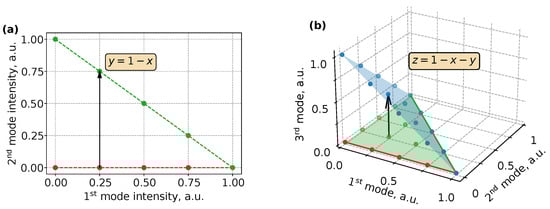
Figure 1. Schematic visualization of the mode enumeration algorithm for the case of two (a) and three (b) modes with five possible intensity levels.

In the general case of $M>2$, the set P is the points that have all coordinate components the same as the points in the set P associated with $M-1$ modes, but whose last coordinate component runs values from zero to maximal (as long as $v_1+v_2+\cdots +v_M\le 1$ is satisfied), i.e.,

$$P(M,n)=\{\{v_1,\dots ,v_{M-1},x\}:\overrightarrow{v}\in P(M-1,n),x\in (i_1,i_2,\dots ,1-\sum _{k=1}^{M-1}{v}_k)\}.$$

(5)

In the following, this algorithm will be used further to compare different mode decomposition methods in absolutely equal initial conditions.

3. Parallel Mode Decomposition Methods Principle

The typical MD setup consists of an SLM, a lens that acts as a Fourier processor, and a CCD camera for recording the output transverse intensity distribution [11]. Here, we simulate the beam from a set of amplitudes, multiply it to a phase transmission function, and compute the two-dimensional Fourier transform to take the intensity distribution in a camera plane. Next, we apply a retrieval procedure and compare the results and initial values.

The propagating laser beam $U\left(\overrightarrow{r}\right)$ at the output of a multimode fiber can be represented as a sum of orthogonal normalized modes ${\psi }_m$ with some complex coefficients $c_m$ (complex amplitudes):

$$U=\sum _m{c}_m{\psi }_m,$$

(6)

where $c_m={\rho }_m{e}^{i{\varphi }_m}$. Due to orthonormalization, the mode amplitude $c_m$ is equal to a simple scalar product:

$$c_m=⟨U\left(\overrightarrow{r}\right)|\psi \left(\overrightarrow{r}\right)⟩.$$

(7)

For a mode decomposition to be possible, it is crucial that this operation can be carried out in a fully optical way. Moreover, there are several algorithms to do this simultaneously for a set of modes using an SLM, which represent a diffraction optical element (DOE). The laser beam $U\left(\overrightarrow{r}\right)$ falls on a DOE with a transmission function $T\left(\overrightarrow{r}\right)$ recorded in it. In the general case, the field E immediately after the DOE will have the following form:

$$E\left(\overrightarrow{r}\right)=U\left(\overrightarrow{r}\right)T\left(\overrightarrow{r}\right).$$

(8)

The field $E\left(\overrightarrow{r}\right)$ passes through the lens and is focused in the focal plane. It is a well-known fact that the field in the focal plane will be proportional to the Fourier image $E_f$ of the original field E:

$$E_f\left(\overrightarrow{r_f}\right)\propto \mathcal{F}\left[E\left(\overrightarrow{r}\right)\right]\left(\overrightarrow{v}\left(\overrightarrow{r_f}\right)\right),$$

(9)

where $\overrightarrow{v}$ is the coordinates in the frequency space (transverse component of wave vectors) and $\overrightarrow{r_f}$ is the coordinates in the focal plane. The coordinates in the focal plane $\overrightarrow{r_f}$ and the coordinates in the frequency space $\overrightarrow{v}$ are geometrically uniquely related, namely:

$$\overrightarrow{r_f}=f\frac{\overrightarrow{v}}{\sqrt{k^2-v^2}},$$

(10)

where f is the focal distance of the lens and $k=2\pi \lambda$ is the modulus of the wave vector. Therefore, only the coordinates in the frequency space $\overrightarrow{v}$ are used below for convenience.

$$E_f\left(\overrightarrow{v}\right)=A_0\mathcal{F}\left[E\left(\overrightarrow{r}\right)\right]\left(\overrightarrow{v}\right),$$

(11)

where $A_0$ is a constant.

Thus, the objective of the mode decomposition method is to obtain the result of expression (7) in a fully optical way by generating a hologram with an appropriate transmission function $T\left(\overrightarrow{r}\right)$. Next, we will briefly describe three different approaches.

3.1. Conjugate Symmetric Extension

The CSE method [20] is based on the conjugate symmetric extension property [22]. The method starts from a block mode matrix that is compiled for several modes ${\psi }_m$. For example, the symmetric conjugate extension $M_{CSE}$ of a matrix M, made of three elements $A,B,C$, i.e.,

$$M=\left(\begin{array}{c}\begin{array}{|c|}\hline A\\ \hline\end{array}\\ \begin{array}{|c|}\hline B\\ \hline\end{array}\\ \begin{array}{|c|}\hline C\\ \hline\end{array}\end{array}\right),$$

(12)

is constructed by attaching to the matrix M and its conjugate copy reflected along both axes, i.e.,

(13)

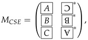where ‘${}^{*}$’ means conjugation.

The elements of the discrete Fourier transform of a matrix of this form $F=\mathcal{F}\left[M_{\mathrm{CSE}}\right]$ are real numbers. The trick is that F is written to the phase-only SLM, so that the transmission function in Equation (24) takes the form $T=exp\left(iH\right)$, where H is F scaled into the range $(-\pi ,\pi )$, as follows:

$$H=2\pi \frac{F-F_{\min }}{F_{\max }-F_{\min }}.$$

(14)

An example of such a phase mask is depicted in Figure 2a.

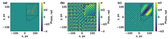
Figure 2. Phase masks for different mode decomposition methods (a) CSE, (b) DPH, (c) PCF to simultaneous measurement amplitudes of six modes.

Let us try to imagine the essence of the process of mode decomposition. The experimental setup consists of a 4f system with the SLM placed in the Fourier plane. When the initial field of a laser beam U is focused by the Fourier lens onto the modulator, the field immediately after reflection from the SLM will have the form:

$$E_{\mathrm{SLM}}=\mathcal{F}\left[U\right]F.$$

(15)

During further propagation, after passing through the Fourier lens, the field is expressed as follows:

$$E_{\mathrm{out}}={\mathcal{F}}^{-1}\left[E_{\mathrm{SLM}}\right]={\mathcal{F}}^{-1}\left[\mathcal{F}\left[U\right]F\right]=U\ast {\mathcal{F}}^{-1}\left[F\right],$$

(16)

where ‘∗’ means convolution. Thus, the intensity distribution in the camera plane (depicted in Figure 3a) can be expressed in the following way:

$$I(x,y)={\left|E_{\mathrm{out}}\right|}^2={\left|(U\ast M_{\mathrm{CSE}})(x,y)\right|}^2.$$

(17)

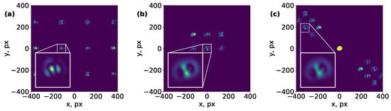
Figure 3. Calculated images in the camera plane for different mode decomposition methods (a) CSE, (b) DPH, (c) PCF to simultaneous measurement of six modes with nearly equal amplitudes.

This implies that the output field contains the convolutions of the original field with each block of the matrix $M_{\mathrm{CSE}}$. One of them is enlarged and presented as an inset in Figure 3a. Using the definition of convolution, it can be shown that at certain coordinates x and y the field $E_{\mathrm{out}}(x,y)$ will be equal to the scalar product of $U(x,y)$ and the mode $A(x,y)$. For other modes, the same will happen in other coordinates. Thus, by collecting the intensity in all those peculiar points, it is possible to obtain the amplitude of all modes simultaneously.

3.2. Double-Phase Hologram

As mentioned before, most of the MD tools rely on phase-only devices. Although these do not permit the direct modulation of the mode amplitude of a beam, it is possible to encode phase patterns to a multimode beam and still retrieve its amplitude-phase mode distribution [19,23]. To this goal, it is useful to define a macropixel as a 2 × 2 array of four real pixels of the SLM screen. In this case, the real transmittance function of a macropixel is the sum of the ideal amplitude-phase transmittance function $T_{nm}$ for this macropixel and a noise term, i.e.,

$$e^{i{\varphi }_{nm}^{1,2,3,4}}=T_{nm}+(e^{i{\varphi }_{nm}^{1,2,3,4}}-T_{nm}).$$

(18)

Note that here we are using a stepped form of the function T, where the transmittance of the macropixel with index $(n,m)$ is $T_{nm}$. The basic idea of the method is to reduce the contribution of the noise term to the zeroth order of diffraction (near the optical axis of the lens) with a proper selection of additive phases at each of the four pixels. The transmission function $T_{nm}$ of a macropixel is expressed as:

$$T_{nm}=\frac{1}{4}(e^{i{\varphi }_{nm}^1}+e^{i{\varphi }_{nm}^2}+e^{i{\varphi }_{nm}^3}+e^{i{\varphi }_{nm}^4}).$$

(19)

The phase shifts $\left\{\varphi \right\}$ are chosen symmetrically here because this results in a symmetric noise distribution about the axis and, as a consequence, in a high signal-to-noise ratio (SNR) in the zero-order diffraction region:

$${\varphi }_{nm}^1={\varphi }_{nm}^4={\varphi }_{nm}^{\left(a\right)},{\varphi }_{nm}^2={\varphi }_{nm}^3={\varphi }_{nm}^{\left(b\right)}.$$

(20)

From here, using the expression, one can obtain the final equations:

$$\begin{array}{c}\hfill {\varphi }_{nm}=arg\left(T_{nm}\right),\end{array}$$

(21)

$$\begin{array}{c}\hfill {\Delta }_{nm}={cos}^{-1}\left(\right|T_{nm}\left|\right),\end{array}$$

(22)

where ${\varphi }_{nm}$ is the average phase of the macropixel with index $(n,m)$ and ${\Delta }_{nm}$ is the phase deviation inside it. It can be shown that the following modification of expression (22) leads to a higher SNR [23]:

$${\Delta }_{nm}={(-1)}^{n+m}{cos}^{-1}\left(\right|T_{nm}\left|\right).$$

(23)

This happens because the sign of ${\Delta }_{nm}$ does not affect the signal component, but leads to the appearance of the phase multiplier $e^{i(n+m)\pi }$ in the noise term, which is equivalent to an additional high-periodic component of the hologram on which strong diffraction occurs.

The final hologram (see Figure 2b) is obtained from the amplitude-phase function $T_{nm}$ by applying Equations (20), (21), and (23). An example of a captured image is shown in Figure 3b together with an enlarged area for one mode presented in the inset.

It should be mentioned that, despite the obvious advantage of the method in the form of simulation of amplitude-phase modulation, there is still a significant disadvantage associated with a decrease in resolution by a factor of four. This is due to the fact that four physical pixels of the modulator are equivalent to one pixel of the encoded amplitude-phase mask.

3.3. Spatial Correlation Filter Based on Jacobi–Anger Expansion

In this last method, the amplitude-phase transmission function from [18] is written into a pure phase hologram, forming a phase correlation filter (PCF), as shown in [24]. As a result, in the first-order diffraction after the Fourier lens, one obtains the convolutions of the laser beam with the Fourier images of the modes of interest, separated by distances that are defined by introducing an addition of carrier frequencies.

MD of a multimode light beam is possible using the SCF method, where a diffraction element with an amplitude-phase transmission function is used for decomposition [18]. This function has the form:

$$T\left(\overrightarrow{r}\right)=\sum _m{\psi }_m^{*}{e}^{i\overrightarrow{V_m}\overrightarrow{r}}.$$

(24)

Using the convolution theorem and relation (8) we can rewrite Equation (11) as follows:

$$E_f\left(\overrightarrow{v}\right)=A_0(\mathcal{F}\left[U\right]\ast \mathcal{F}\left[T\right])\left(\overrightarrow{v}\right).$$

(25)

Due to the fact that the modes have been written with slightly different carrier frequencies $\overrightarrow{V_m}$ in the transmission function (24), the field $E_f$ will contain terms of the form:

$$K\left(\overrightarrow{v}\right)=[\mathcal{F}\left[U\right]\left(\overrightarrow{t}\right)\ast \mathcal{F}{\psi }_m^{*}(\overrightarrow{t}-\overrightarrow{V_m})]\left(\overrightarrow{v}\right).$$

(26)

The convolutions (26) at the correct choice of carrier frequencies $\overrightarrow{V_m}$ will not overlap with each other in the frequency space. In the center of each convolution (from the property of the Fourier transform) we obtain the following scalar product:

$$E_f\left(\overrightarrow{V_m}\right)=A_0⟨U\left(\overrightarrow{r}\right)|\psi \left(\overrightarrow{r}\right)⟩\propto c_m.$$

(27)

The transmission function $T\left(\overrightarrow{r}\right)$ described above can be written in pure phase form through the Jacobi–Anger expansion [24]. The function $T\left(\overrightarrow{r}\right)$ is then treated as a signal to be recorded in the hologram (depicted in Figure 2c). All convolutions defined by Equation (26) will shift by another common carrier frequency into the first order of diffraction. Thus, by measuring the field intensity at the center of the correlation signals $|K\left(\overrightarrow{v}\right){|}^2$ in the focal plane, one can determine $|c_m{|}^2$, which is the square of the amplitude of the m-th mode.

Then, in order to determine the mode phase ${\varphi }_m$, i.e., the argument of the coefficient $c_m$, it is necessary to add specially defined terms to the sum in Equation (24) [18]. Note that the mode phases are defined with respect to a reference value. Usually, this is taken in such a way that the fundamental mode (${\varphi }_0$) has zero phase. To determine the cosine of the phase shift ${\varphi }_m-{\varphi }_0$ of mode ${\psi }_m$ we need a term of the form:

$$T_m^{cos}\left(\overrightarrow{r}\right)=\frac{1}{\sqrt{2}}({\psi }_0^{*}+{\psi }_m^{*})e^{i{\overrightarrow{V}}_m^{cos}\overrightarrow{r}}.$$

(28)

Whereas the following term is needed to determine the sine of the same phase shift:

$$T_m^{sin}\left(\overrightarrow{r}\right)=\frac{1}{\sqrt{2}}({\psi }_0^{*}+i{\psi }_m^{*})e^{i{\overrightarrow{V}}_m^{sin}\overrightarrow{r}}.$$

(29)

The correlation signals corresponding to these terms will also be separated according to the selected carrier frequencies ${\overrightarrow{V}}_m^{cos}$ and ${\overrightarrow{V}}_m^{sin}$ (see Figure 3c).

4. Results

All methods were applied to beams made of either $M=3$, 6, or 10 modes. We computed the correlation between the set and the retrieved amplitudes for all possible mode combinations, as described in Section 2. In particular, for the case of three modes, we used $n=9$ intensity levels. According to Equation (3), $M=3$ and $n=9$ result in 45 combinations, henceforth frames. In contrast, in the cases of six and ten modes, we considered $n=12$ intensity levels, which led to 4368 and 167,960 frames, respectively. For each frame, the correlation was calculated as the dot product of the initial amplitude vector and retrieved amplitude vector. The results are shown in Figure 4, Figure 5 and Figure 6. As can be seen, the correlation values always stay on a relatively high level: the minimum value reached for the CSE method, is close to 96%, whereas PCF and DPH are associated with correlation values close to 100%. Interestingly, some outlier values of correlation arise in the CSE method when the beam consists primarily of one mode. In contrast, nearly monomode beams are not so critical for the other two methods.

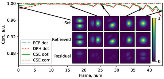
Figure 4. The simulated real-time MD results applied to $M=3$ mode beams considering $n=9$ intensity levels. The insets depict the intensities of the set (initial), retrieved, and residual beams of a few frames, which are indicated by arrows.

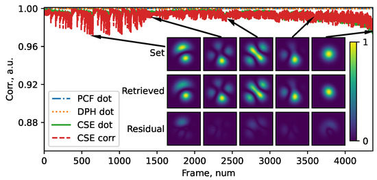
Figure 5. Same as Figure 4 with $M=6$ and $n=12$.

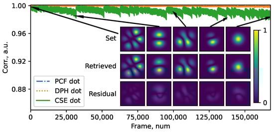
Figure 6. Same as Figure 4 with $M=10$ and $n=12$.

One may notice that, because the initial mode amplitude is unknown, in real experiments there is no opportunity to verify the correctness of the MD as described above. Therefore, for the sake of completeness, here we mimic the test of an experimental MD validity by calculating the cross-correlation parameter [25]. The latter, which allows us to compare two images (initial and reconstructed), is defined as

$$C=\frac{{\sum }_{mn}(A_{mn}-\overline{A})(B_{mn}-\overline{B})}{\sqrt{{\sum }_{mn}{(A_{mn}-\overline{A})}^2{\sum }_{kl}{(B_{kl}-\overline{B})}^2}},$$

(30)

where $\overline{A}$ and $\overline{B}$ are the mean values of the matrices A and B, respectively, whose elements are $A_{mn}$ and $B_{mn}$, respectively. Here, the matrices represent pixelated frames containing initial and reconstructed beams. The cross-correlation parameter was calculated for the CSE method in the case of three and six modes (red line in Figure 4 and Figure 5). As can be seen, we found a similar behavior to that of the amplitude correlation calculated via the dot product (green line). This agreement allowed us to conclude that the CSE method is less accurate than DPH and PCF. Still, it has to be underlined that the CSE’s accuracy remains comparable to that of methods based on neural networks [26].

Finally, in order to make a graphical comparison of the three methods used in this work, in Figure 7 we plot on a logarithmic scale the resulting mismatch for all cases reported in Figure 4, Figure 5 and Figure 6. Specifically, on the horizontal axis of the figure we put the standard deviation, which characterizes the scatter of values in the target intensity set: the smaller the standard deviation, the smaller the error.

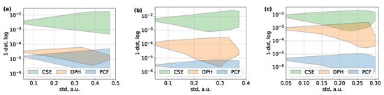
Figure 7. Comparison of inaccuracies for different mode decomposition methods to simultaneous measurement of (a) three, (b) six, (c) ten modes for all combinations of input amplitudes.

In addition to demonstrating once again that CSE is the least accurate of the three methods, the graphs allow us to conclude that, for all methods, the error increases as the number of modes grows larger. This is most noticeable for the DPH method, where the discrepancy increases by an order of magnitude when passing from $M=3$ to $M=10$. As mentioned above, this effect may be ascribed to the four-fold decrease in the resolution of DPH in comparison with other methods.

5. Conclusions

In this work, we performed a numerical comparison of different MD methods based on digital holography that allows real-time measurements for a set of modes. First, by means of an enumeration algorithm, we searched for all possible modal content combinations for a predefined number of modes and amplitude levels. To the best of our knowledge, such an approach has never been explored before. Three methods (CSE, DPH, and PCF) were numerically implemented and compared. Our results allowed us to conclude that, among the three, the CSE method is the least accurate, albeit comparable to the deep learning techniques; the DPH method also presented a major drawback: its resulting mismatch grows with the number of modes. Thus, the most useful method turned out to be that based on PCF with the use of the Jacobi–Anger expansion. We believe that the results of this research will be useful in the experimental investigation of fast mode dynamics and temporal instabilities in MM fiber lasers and amplifiers as well as for the demonstration of real-time MD devices, which are cutting-edge tools owing to the great attention given to the investigation of multimode fiber systems. Moreover, the MD methods considered in this work are independent of the carrier wavelength and can in principle be used in completely different ranges, e. g., for the analysis of terahertz radiation [27,28]. In addition, the development of a robust and reliable MD device will facilitate research using multimode fibers in areas such as optical rogue waves [29] and quantum multimode dynamics in a wide range of materials [30].

References

- Cristiani, I.; Lacava, C.; Rademacher, G.; Puttnam, B.J.; Luìs, R.S.; Antonelli, C.; Mecozzi, A.; Shtaif, M.; Cozzolino, D.; Bacco, D.; et al. Roadmap on multimode photonics. J. Opt. 2022, 24, 083001. [Google Scholar] [CrossRef]
- Dianov, E.M.; Prokhorov, A.M. Medium-power CW Raman fiber lasers. IEEE J. Sel. Top. Quantum Electron. 2000, 6, 1022–1028. [Google Scholar] [CrossRef]
- Yao, T.; Harish, A.V.; Sahu, J.K.; Nilsson, J. High-power continuous-wave directly-diode-pumped fiber Raman lasers. Appl. Sci. 2015, 5, 1323–1336. [Google Scholar] [CrossRef]
- Glick, Y.; Shamir, Y.; Sintov, Y.; Goldring, S.; Pearl, S. Brightness enhancement with Raman fiber lasers and amplifiers using multi-mode or multi-clad fibers. Opt. Fiber Technol. 2019, 52, 101955. [Google Scholar] [CrossRef]
- Li, L.; Leng, J.; Zhou, P.; Chen, J. Multimode fiber modal decomposition based on hybrid genetic global optimization algorithm. Opt. Express 2017, 25, 19680. [Google Scholar] [CrossRef] [PubMed]
- Flamm, D.; Naidoo, D.; Schulze, C.; Forbes, A.; Duparré, M. Mode analysis with a spatial light modulator as a correlation filter. Opt. Lett. 2012, 37, 2478. [Google Scholar] [CrossRef] [PubMed]
- An, Y.; Huang, L.; Li, J.; Leng, J.; Yang, L.; Zhou, P. Deep Learning-Based Real-Time Mode Decomposition for Multimode Fibers. IEEE J. Sel. Top. Quantum Electron. 2020, 26, 4400806. [Google Scholar] [CrossRef]
- Jiang, M.; An, Y.; Su, R.; Huang, L.; Li, J.; Ma, P.; Ma, Y.; Zhou, P. Deep Mode Decomposition: Real-Time Mode Decomposition of Multimode Fibers Based on Unsupervised Learning. IEEE J. Sel. Top. Quantum Electron. 2022, 28, 4400806. [Google Scholar] [CrossRef]
- Krupa, K.; Tonello, A.; Shalaby, B.M.; Fabert, M.; Barthelemy, A.; Millot, G.; Wabnitz, S.; Couderc, V. Spatial beam self-cleaning in multimode fibres. Nat. Photonics 2017, 11, 237–241. [Google Scholar] [CrossRef]
- Mangini, F.; Gervaziev, M.; Ferraro, M.; Kharenko, D.S.; Zitelli, M.; Sun, Y.; Couderc, V.; Podivilov, E.V.; Babin, S.A.; Wabnitz, S. Statistical mechanics of beam self-cleaning in GRIN multimode optical fibers. Opt. Express 2022, 30, 10850. [Google Scholar] [CrossRef]
- Gervaziev, M.; Ferraro, M.; Podivilov, E.V.; Mangini, F.; Sidelnikov, O.S.; Kharenko, D.S.; Zitelli, M.; Fedoruk, M.P.; Babin, S.A.; Wabnitz, S. Mode Decomposition Method for Investigating the Nonlinear Dynamics of a Multimode Beam. Optoelectron. Instrum. Data Process. 2023, 59, 51–61. [Google Scholar] [CrossRef]
- Ferraro, M.; Mangini, F.; Zitelli, M.; Wabnitz, S. On spatial beam self-cleaning from the perspective of optical wave thermalization in multimode graded-index fibers. Adv. Phys. X 2023, 8, 1–35. [Google Scholar] [CrossRef]
- Stutzki, F.; Otto, H.J.; Jansen, F.; Gaida, C.; Jauregui, C.; Limpert, J.; Tünnermann, A. High-speed modal decomposition of mode instabilities in high-power fiber lasers. Opt. Lett. 2011, 36, 4572. [Google Scholar] [CrossRef]
- Otto, H.J.; Stutzki, F.; Jansen, F.; Eidam, T.; Jauregui, C.; Limpert, J.; Tünnermann, A. Temporal dynamics of mode instabilities in high-power fiber lasers and amplifiers. Opt. Express 2012, 20, 15710. [Google Scholar] [CrossRef]
- Tao, R.; Wang, X.; Zhou, P. Comprehensive Theoretical Study of Mode Instability in High-Power Fiber Lasers by Employing a Universal Model and Its Implications. IEEE J. Sel. Top. Quantum Electron. 2018, 24, 0903319. [Google Scholar] [CrossRef]
- Jauregui, C.; Stihler, C.; Limpert, J. Transverse mode instability. Adv. Opt. Photonics 2020, 12, 429. [Google Scholar] [CrossRef]
- Distler, V.; Möller, F.; Yildiz, B.; Plötner, M.; Jauregui, C.; Walbaum, T.; Schreiber, T. Experimental analysis of Raman-induced transverse mode instability in a core-pumped Raman fiber amplifier. Opt. Express 2021, 29, 16175. [Google Scholar] [CrossRef] [PubMed]
- Kaiser, T.; Flamm, D.; Schröter, S.; Duparré, M. Complete modal decomposition for optical fibers using CGH-based correlation filters. Opt. Express 2009, 17, 9347. [Google Scholar] [CrossRef] [PubMed]
- Hsueh, C.K.; Sawchuk, A.A. Computer-generated double-phase holograms. Appl. Opt. 1978, 17, 3874. [Google Scholar] [CrossRef] [PubMed]
- Zhao, Y.; Huang, S.; Yan, C. Parallel measurement of multiple linear polarization modes in few-mode optical fibers using spatial light modulators. Opt. Eng. 2019, 58, 1. [Google Scholar] [CrossRef]
- Flajolet, P.; Sedgewick, R. Analytic Combinatorics; Cambridge University Press: Cambridge, UK, 2009. [Google Scholar]
- Huang, S.J.; Wang, S.Z.; Yu, Y.J. Computer generated holography based on Fourier transform using conjugate symmetric extension. Acta Phys. Sin. 2009, 58, 952–958. [Google Scholar] [CrossRef]
- Arrizón, V.; Sánchez-de-la Llave, D. Double-phase holograms implemented with phase-only spatial light modulators: Performance evaluation and improvement. Appl. Opt. 2002, 41, 3436. [Google Scholar] [CrossRef]
- Arrizón, V.; Ruiz, U.; Carrada, R.; González, L.A. Pixelated phase computer holograms for the accurate encoding of scalar complex fields. J. Opt. Soc. Am. A 2007, 24, 3500. [Google Scholar] [CrossRef]
- Schulze, C.; Schmidt, O.A.; Flamm, D.; Duparré, M.; Schröter, S. Modal analysis of beams emerging from a multi-core fiber using computer-generated holograms. Fiber Lasers VIII Technol. Syst. Appl. 2011, 7914, 79142H. [Google Scholar]
- An, Y.; Huang, L.; Li, J.; Leng, J.; Yang, L.; Zhou, P. Learning to decompose the modes in few-mode fibers with deep convolutional neural network. Opt. Express 2019, 27, 10127. [Google Scholar] [CrossRef]
- Jin, Q.; Yiwen, E.; Gao, S.; Zhang, X.C. Preference of subpicosecond laser pulses for terahertz wave generation from liquids. Adv. Photonics 2020, 2, 1–6. [Google Scholar] [CrossRef]
- Zhang, Z.; Zhang, J.; Chen, Y.; Xia, T.; Wang, L.; Han, B.; He, F.; Sheng, Z.; Zhang, J. Bessel Terahertz Pulses from Superluminal Laser Plasma Filaments. Ultrafast Sci. 2022, 2022, 9870325. [Google Scholar] [CrossRef]
- Song, Y.; Wang, Z.; Wang, C.; Panajotov, K.; Zhang, H. Recent progress on optical rogue waves in fiber lasers: Status, challenges, and perspectives. Adv. Photonics 2020, 2, 32–34. [Google Scholar] [CrossRef]
- Guan, M.; Chen, D.; Hu, S.; Zhao, H.; You, P.; Meng, S. Theoretical Insights into Ultrafast Dynamics in Quantum Materials. Ultrafast Sci. 2022, 2022, 9767251. [Google Scholar] [CrossRef]
Disclaimer/Publisher’s Note: The statements, opinions and data contained in all publications are solely those of the individual author(s) and contributor(s) and not of MDPI and/or the editor(s). MDPI and/or the editor(s) disclaim responsibility for any injury to people or property resulting from any ideas, methods, instructions or products referred to in the content. |
© 2023 by the authors. Licensee MDPI, Basel, Switzerland. This article is an open access article distributed under the terms and conditions of the Creative Commons Attribution (CC BY) license (https://creativecommons.org/licenses/by/4.0/).