Abstract
Atmospheric turbulence causes signal beam wavefront distortion at the receiving end of a coherent detection system, which decreases the system mixing efficiency. Based on the coherent detection theory, this study establishes a mathematical model of wavefront distortion with mixing efficiency and mixing gain. It also analyzes the improvement limits of wavefront correction on mixing efficiency and mixing gain under different atmospheric turbulence intensities and experimentally measures them. Simulation results show that the mixing efficiency can be improved to 51%, 55%, and 60% after correcting for tilt, defocus, and astigmatism terms, respectively, when turbulence intensity D/r0 is 2. The mixing gain with homodyne detection is 3 dB higher than heterodyne detection. Meanwhile, the wavefront correction orders required for optimal mixing efficiency are higher than the heterodyne correction order. In the experiment, Haso4 NIR + DM 40 was used, and the turbulence intensity D/r0 was 2. After the closed-loop control algorithm corrects the tilt, defocus, and astigmatism terms, the indoor experimental results showed that the mixing efficiency is improved to 36%, 47%, and 62%, respectively. The outdoor experimental results showed that the mixing efficiency improved to 36%, 51%, and 68%, respectively.
1. Introduction
Coherent detection is a key technology for improving the reception sensitivity of optical wireless coherent communication systems [1,2]. An optical wireless coherent communication system includes two detection methods: heterodyne and homodyne [3,4]. The distortion of the signal light wavefront caused by atmospheric turbulence and other factors destroys the spatial phase matching between the signal light and local oscillation light at the receiving end, leading to a decrease in the coherent detection efficiency at the receiving end [5]. This severely affects optical wireless coherent communication.
To suppress the effect of wavefront distortion caused by atmospheric turbulence and other factors on communication performance, Banakh et al. analyzed the feasibility of compensating for the wavefront distortion of a beam when using aperture detection for laser sources of different wavelengths. The results demonstrated that the maximum compensation time for wavefront distortion was achieved within 3 to 3.5 s with the help of a reflector-controlled signal beam [6]. Lejia et al. proposed a Shack–Hartmann wavefront sensor that detected high-order wavefront distortion. This wavefront sensor’s root mean square error was reduced by 40.54%, and the Strehl ratio was improved by 27.31% compared with a mode-based conventional wavefront sensor [7]. Zhang Zhentao et al. proposed a method of tilt measurement using only a plenoptic wavefront sensor and built an experimental platform to verify the tilt measurement accuracy and closed-loop wavefront correction performance. The experimental results show that the Strehl ratio after wavefront correction is increased by 40%, which proves the feasibility of using an all-optical wavefront sensor in a closed-loop adaptive optics (AO) system [8]. Rani N et al. proposed to combine homodyne detection with multi-beam technology to achieve the purpose of reducing the scintillation effect. The research results show that, under the condition of the transmission distance of 4.5 km, the multi-beam system using homodyne detection can detect the laser power at −3 dBm, and realize the detection of weak signals [9]. Yan Xu et al. proposed a system for dynamic detection of wavefront distortion using signal light nutation and performed wavefront compensation analysis. The simulation results show that when the atmospheric turbulence intensity D/r0 = 15, the wavefront root mean square (RMS) value drops to 0.0042 after wavefront correction, which has higher wavefront compensation accuracy [10]. Zhong ZQ et al. proposed a laser beam using a self-rotating wavefront to eliminate the degradation caused by turbulence and obtain a lower peak-to-valley (PV) [11]. Among them, the introduction of AO technology further improved the mixing efficiency at the receiver side of the system, becoming an effective method to suppress the atmospheric turbulence effect [12,13,14]. The AO system corrected by the Zernike mode method can effectively compensate for the wavefront distortion effect caused by atmospheric turbulence on the reception sensitivity of the optical wireless coherent communication system [15,16,17,18]. For the correction compensation of the wavefront distortion of the coherent detection system at the receiver side [19,20], the under-compensation of the wavefront distortion leads to a loss of the coherent detection system performance. In contrast, the over-compensation increases the system complexity and algorithm redundancy. Therefore, both under and over-correction compensation of wavefront distortion in coherent detection systems have limitations when exploring the wavefront distortion’s impact on the performance of coherent detection systems. In addition to analyzing the pattern of wavefront distortion, the effect of each wavefront distortion and its correction on the performance at the receiver are important factors in achieving optimal mixing. Furthermore, the performance limits of coherent detection systems place higher demands on the order of wavefront distortion correction.
Here, we consider the mixing efficiency and mixing gain of a coherent detection system as the evaluation index to establish a theoretical model of wavefront distortion caused by atmospheric turbulence. The wavefront distortion influence on the system’s mixing efficiency by classification was discussed. In addition, the improvement limit of wavefront correction on mixing efficiency, and gain were comprehensively considered. Finally, combined with theoretical simulations and experimental studies, theoretical and experimental bases were provided for applying the AO technology to a coherent detection system.
2. Theoretical Research
2.1. Coherent Detection Principle
The principle of the coherent detection system is illustrated in Figure 1 [21]. Based on the theory of atmospheric turbulence, the mixing efficiency was used as an evaluation index after the coherent detection of the signal light and local oscillation light at the receiver end of the system.

Figure 1.
Coherent detection principle diagram.
Let the optical fields of the signal light and local oscillation light be denoted as [22]:
In Equations (1) and (2), As, ωs, and φs are the signal light amplitude, angular frequency, and phase, respectively; Al, ωl, and φl are the local oscillation light amplitude, angular frequency, and phase, respectively. The incident light power of the system is expressed as [23]:
where k is a proportionality constant, S is the incident field area of the photodetector, and |*| denotes the modulo operation on *. By substituting Equations (1) and (2) into Equation (3), the incident optical power can be expressed as:
where Δω = ωs-ωl and Δφ = φs-φl, and the intermediate-frequency current iIF through the detector is expressed as [24]:
In Equation (5), R is the photodetector sensitivity, which can be expressed as:
where e is the unit electron charge, η is the quantum efficiency of the photodetector, h is Planck’s constant, and v is the carrier frequency. According to Equation (5), we obtain:
where ⟨ ⟩ denotes average system synthesis. For a coherent detection system, the scattered particle noise caused by the local oscillation light is much larger than other noises, and it can be assumed that the noise at the receiver side mainly originates from the local oscillation light [25]:
where Il is the local-oscillation photocurrent, B = 2Δf, Δf is the effective noise bandwidth, Pl is the power of the local-oscillation light. Then, according to Equations (7) and (8), the output signal-to-noise ratio (SNR) can be expressed as:
where Ps is the power of the signal light. Then, the mixing efficiency of the heterodyne detection can be expressed as:
When the mixing efficiency reaches the ideal extreme value, Then, Equation (9) can be simplified as:
Equation (11) is expressed as the theoretical detection limit of optical wireless coherent detection [5]. When the frequency of the local oscillation light is equal to the signal light frequency, it is called homodyne detection [26,27], and Equation (5) becomes:
Subsequently, the homodyne detection mixing efficiency is expressed as:
Combining Equations (10) and (13), the mixing gain is defined as:
The mixing gain can measure the mixing efficiency improvement times after wavefront correction (dB).
2.2. Phase Wavefront Distortion
The phase mismatch becomes increasingly severe owing to turbulence effects in the channel [28]. The wavefront distortion from the phase mismatch is described by the Zernike polynomial as follows [29]:
where (r,θ) is the polar coordinate in the circular domain; N is the number of Zernike terms; ai is the coefficient of the i-th Zernike polynomial. We refer to the mean square parameter associated with the wavefront coefficient as the distortion amplitude, and Zi is the i-th Zernike polynomial, which can be expressed as [30]:
In Equation (16), n is the order of the Zernike polynomial; m is the angular frequency; n and m are integers satisfying m ≤ n, n-|m| = even; Zodd·i corresponds to the mode term containing sinmθ; Zeven·i corresponds to the mode term containing cosmθ; and the radial polynomial containing (r) is expressed as:
The Zernike coefficients ai must be determined using a diagonalization algorithm that describes the process of simulating the wavefront distortion; ai can be solved from the covariance matrix. For the wavefront phase coefficient vector A = [a1, a2, …, an]T, the covariance matrix C can be written as [29]:
In the covariance matrix C, the covariance expressions for the Zernike polynomials Zi and Zj are:
where E(*) represents the covariance operator of the random variable, the ratio of receiving aperture D to the atmospheric coherence length r0 represents turbulence intensity D/r0, and the covariance cij is expressed as [30]:
where ni, mi, mj, and mj are the Zernike polynomial order and angular frequency numbers corresponding to ai and aj, respectively; q is the parameter of the Bessel integral function; Jn+1(*) is the first-class n + 1 order Bessel function, and x belongs to the set of real numbers. δmimj is the Kronecker function, expressed as:
In Equation (20), the Bessel indefinite integral function defined by Weber is solved to obtain [31]:
where Γ(*) denotes the gamma function. Substituting Equation (22) into Equation (20), cij can be expressed as:
According to Equation (18), the Zernike polynomials do not satisfy the statistical independence when the covariance array is not zero. Therefore, the Karhunen–Loeve polynomial was introduced to expand the wavefront and construct random quantities with specific variances [32]. Wavefront distortion is described by the Karhunen–Loeve polynomial as follows:
where bj is a statistically independent random coefficient, and Kj(r,θ) is a Karhunen–Loeve polynomial. Subsequently, the Zernike polynomial can be expanded by the Karhunen–Loeve polynomial as:
where Vij is the transition matrix. Therefore, according to Equations (24) and (25), the wavefront distortion can be described as:
Combining with Equation (15), the wavefront coefficient vector A is expressed as:
In Equation (27), vector B = [b1, b2, …, bn]T, V is the Karhunen–Loeve polynomial transformation matrix, and the Zernike coefficients describing the wavefront are obtained by substituting Equation (27) and Equation (15). The resulting wavefront coefficient vector A is multiplied by (D/r0)5/3 to obtain the exact covariance of the Zernike polynomial weights evaluated from the atmospheric spectrum to produce the desired wavefront distortion.
3. Numerical Simulation
3.1. Effect of Wavefront Distortion on Mixing Efficiency
The defocus-spherical distortion class of wavefront distortions includes defocus (Z4), spherical distortion (Z11), and higher-order spherical distortions. This type of wavefront distortion distribution, spatially uncorrelated with the polar angle θ, forms a circularly symmetric feature centered at the origin and is classified as such. Combined with Equation (15) when subjected to defocus-spherical distortion of wavefront class only, the simulation conditions are set to photodetector quantum efficiency η = 0.8, Planck’s constant of h = 6.63 × 10⁻³⁴ J·s, speed of light of c = 2.99 × 10⁸ m/s, a wavelength of λ = 1550 nm, effective noise bandwidth of Δf = 200 MHz, the signal optical power of Ps = 0.36 μW, local oscillation optical power of Pl = 0.36 mW conditions, distortion amplitude in the range of 0–10 λ, and heterodyne detection mixing efficiency with the variation of defocus-spherical distortion amplitude of class. The numerical simulation results are shown in Figure 2.
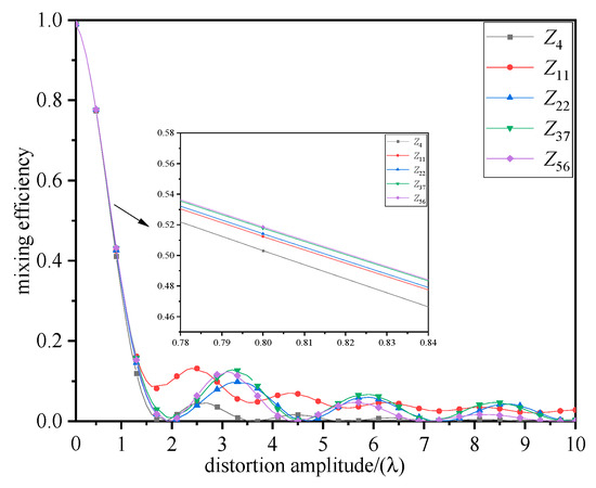
Figure 2.
Relationship between distortion amplitude of defocus-spherical distortion class and heterodyne detection mixing efficiency.
Figure 2 shows simulations to obtain such wavefront distortion, the heterodyne detection mixing efficiency curves show the same overall change trend. Figure 2 shows that when the distortion amplitude was less than 1 λ, the mixing efficiency was the same. With an increase in the distortion amplitude, the mixing efficiency showed different degrees of oscillation decrease. Moreover, because the proportion of the low-order distortion component in the entire wavefront distortion is much larger than that of the high-order distortion component, the wavefront distortion caused by the defocus component (Z4) has the greatest impact on the mixing efficiency, and the impact of the high-order distortion component on the mixing efficiency gradually decreases.
The tilt-coma distortion class of wavefront distortion includes tilt (Z2), coma (Z8), and its higher-order coma. The high-frequency portion of such distortion completely contains the wavefront polar axis r and polar angle θ components with lower spatial frequencies. Only the coefficients of each component are different, making such wavefront distortion superimposed on different levels of coma components based on the tilt term. By selecting the same simulation parameters as shown in Figure 2 and combining them with Equation (15) only subject to tilt-coma distortion class wavefront distortion, the distortion amplitude in the range of 0–10 λ, the variation curve of the heterodyne detection mixing efficiency with distortion amplitude are shown in Figure 3.
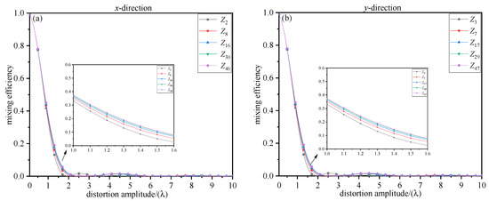
Figure 3.
Relationship between distortion amplitude of tilt-coma distortion class and heterodyne detection mixing efficiency: (a) effect of distortion amplitude in x-direction on mixing efficiency; (b) effect of distortion amplitude in y-direction on mixing efficiency.
Figure 3a shows the variation in the mixing efficiency with the distortion amplitude in x-direction heterodyne detection, and Figure 3b shows the variation in the mixing efficiency with the distortion amplitude in y-direction heterodyne detection. Because the tilt-coma distortion in the x-direction and y-direction only has directional differences, only Figure 3a is analyzed here. In Figure 3a, we observe that the mixing efficiency decays rapidly to 0.4 with increasing distortion amplitude up to 1 λ, and is almost zero when the distortion amplitude is higher than 2 λ. Moreover, because the high-frequency portion of such wavefront distortion completely contains distortion components of low spatial order, however, the coefficients of each component are different, therefore the impact of such wavefront distortion on the mixing efficiency is extremely comparable. In addition, the x-direction tilt distortion (Z2) and y-direction tilt distortion (Z3) had the highest impact on the mixing efficiency.
The astigmatism class wavefront distortion increases with the Zernike order; the polar axis r increases by a power exponent, and the polar angle θ increases by a factor. By selecting the same simulation parameters as those presented in Figure 2, the variation curves of the heterodyne detection mixing efficiency with the amplitude of the astigmatism class distortion in Equation (15) when subjected to only the astigmatism class wavefront distortion in the range of 0–10 λ are illustrated in Figure 4.
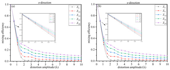
Figure 4.
Relationship between distortion amplitude of astigmatism class and heterodyne detection mixing efficiency: (a) effect of distortion amplitude in x-direction on mixing efficiency; (b) effect of distortion amplitude in y-direction on mixing efficiency.
Figure 4a shows the variation in the heterodyne detection mixing efficiency with the amplitude of the astigmatism class distortion in the x-direction. Figure 4b shows the variation in the heterodyne detection mixing efficiency with the amplitude of the astigmatism class distortion in the y-direction. Owing to the same influence on the trend, only Figure 4a is analyzed here. As shown in Figure 4a, an x-directional astigmatism amplitude of less than 1.3 λ has a greater effect on the decay of the mixing efficiency, and then the decay of the mixing efficiency gradually slows with the increase in the distortion amplitude. In addition, when the distortion amplitude was the same, the higher the order of the astigmatism wavefront distortion, the smaller the effect on the mixing efficiency. Among them, there is also a secondary (Z12, Z13) and high-order astigmatism class in the astigmatism class distortion, which similarly affects the mixing efficiency.
It is concluded that compared with other wavefront distortions, the defocus-spherical distortion class of wavefront distortions has different degrees of oscillation decrease in the mixing efficiency of heterodyne detection with the increase of the distortion amplitude, which is due to this type of wavefront distortion having circular symmetry. However, under the same amount of distortion amplitude, the attenuation of the mixing efficiency by tilt-coma distortion class of wavefront distortion is more obvious than that of other wavefront distortions. Among them, the tilt distortion has the most serious impact on the mixing efficiency, so it is necessary for the tilt distortion of the wavefront distortion to be corrected separately to improve mixing efficiency.
3.2. Evaluation of Mixing Efficiency and Mixing Gain
The influence of the wavefront distortion generated in the atmospheric turbulence on the coherent detection system decreases the mixing efficiency of the coherent detection system with the increase of the turbulence intensity. Therefore, we further analyzed the correction of wavefront distortion for the improvement of the mixing efficiency of the coherent detection system, and with the increase of turbulence intensity, we considered that a larger wavefront correction order is required to compensate for the phase wavefront distortion, to achieve the best compensation for the mixing efficiency and mixing gain of the coherent detection system at the receiving end.
Regarding the correction of wavefront distortion, Zernike polynomials are used to describe the initial wavefront distortion under each specific atmospheric turbulence intensity D/r0, and a 340-order distortion matrix is generated. Wherein, as the wavefront correction order increases, the wavefront distortion is iteratively corrected until the wavefront distortion phase is corrected to a theoretical value of 0, which is the end of the wavefront distortion correction. Then, the influence curve of the order of wavefront correction on the mixing efficiency of the coherent detection system is fitted using a polynomial curve. Figure 5 shows the iterative curve of wavefront distortion correction under a specific turbulence intensity.
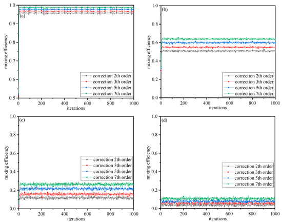
Figure 5.
Iterative curves of wavefront correction and mixing efficiency under different turbulence intensities: (a) D/r0 = 0.2; (b) D/r0 = 2; (c) D/r0 = 5; (d) D/r0 = 8.
Figure 5a–d show that under a certain atmospheric turbulence intensity, as the wavefront correction order increases, the mixing efficiency is improved; and as the atmospheric turbulence intensity increases, the mixing efficiency curve jitters more obviously. This is because the coefficient of wavefront distortion is related to the turbulence intensity D/r0. The greater the intensity of atmospheric turbulence, the more obvious the change of the wavefront distortion coefficient during the correction process, and the more jittery the mixing efficiency presented.
Next, we further discuss the optimal correction order of wavefront distortion required when the performance of the coherent detection system at the receiving end is determined, and the improvement limit of the mixing efficiency with the correction order of wavefront distortion.
When the bit error rate (BER) of the coherent detection system at the receiving end is determined, the simulation conditions are set as follows: receiving aperture D = 105 mm, corresponding to D/r0 is 0.2, 2, 5, and 8; quantum efficiency of the photodetector η = 0.8, Planck’ constant h = 6.63 × 10⁻³⁴ J·s, speed of light c = 2.99 × 10⁸ m/s, wavelength λ = 1550 nm, signal optical power Ps = 0.36 μW, local oscillation optical power Pl = 0.36 mW, and effective noise bandwidth Δf = 200 MHz. For the coherent detection system with specific performance indicators, the optimal wavefront correction order is calculated under different turbulence intensities, and the simulation results are shown in Figure 6.
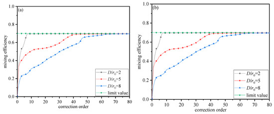
Figure 6.
When the performance of the coherent detection system is determined, the wavefront distortion correction order changes: (a) heterodyne detection; (b) homodyne detection.
When the BER of the coherent detection system at the receiving end is on the order of 10−9, the corresponding mixing efficiency is 0.7. To meet the system performance index, the optimal correction order required is shown in Figure 6. Among them, when observing Figure 6a, it can be concluded that when D/r0 is 2 in heterodyne detection, the correction 10th order mixing efficiency reaches the system requirements; when D/r0 is 5, the correction 59th order mixing efficiency reaches 0.7; when D/r0 is 8, the correction 69th order mixing efficiency is required to reach 0.7; Figure 6b shows the order relationship of wavefront correction to meet the requirements of the coherent detection system in homodyne detection. When D/r0 is 2, 5, and 8, the mixing efficiency of the wavefront correction at the 10th, 61st, and 72nd order reaches 0.7; When the minimum turbulence intensity D/r0 is 0.2, the mixing efficiency after wavefront distortion correction is greater than 0.7.
The simulation conditions were set as follows: receiving aperture D = 105 mm, corresponding to D/r0 of 0.2, 2, 5, and 8; quantum efficiency of the photodetector η = 0.8; Planck’s constant h = 6.63 × 10⁻³⁴ J·s; the speed of light c = 2.99 × 10⁸ m/s; wavelength λ = 1550 nm; signal optical power Ps = 0.36 μW, local oscillation optical power Pl = 0.36 mW, and effective noise bandwidth Δf = 200 MHz. When the wavefront correction order N in Equation (15) changes, the extreme values of the heterodyne detection mixing efficiency calculated using Equation (10) are obtained using numerical calculations. The simulation results are shown in Figure 7.
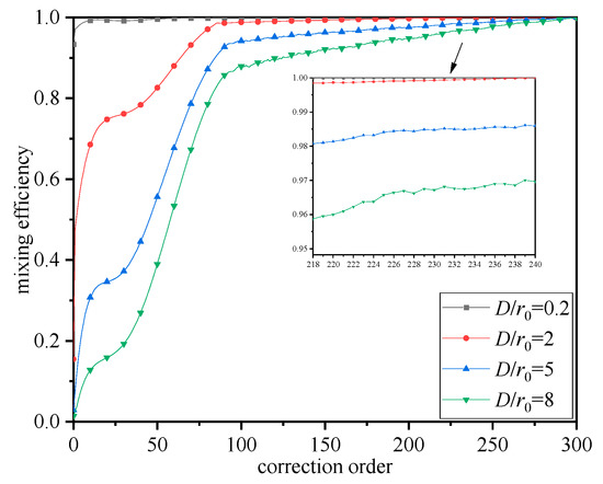
Figure 7.
Relationship between wavefront correction and mixing efficiency in heterodyne detection.
Figure 7 shows that the mixing efficiency is significantly improved for a certain number of wavefront correction orders. The mixing efficiency converges to a stable value by increasing the number of correction orders. Among them, the influence of low-order wavefront correction on the mixing efficiency is obvious. The corresponding mixing efficiency increases to 97%, 51%, 12%, and 4% when D/r0 is 0.2, 2, 5, and 8, respectively, and only the tilt term is corrected. Following the correction of the defocus term, the mixing efficiency increases to 98%, 55%, 16%, and 6%; following the correction of the astigmatism term, the mixing efficiency increases to 99%, 60%, 22%, and 8%. When D/r0 is 0.2 in the heterodyne detection, only the 5th-order wavefront correction is completed, and the mixing efficiency reaches the extreme value. When D/r0 is 2, the correction 85th order mixing efficiency reaches the extreme value. When D/r0 is 5, the mixing efficiency below 231 orders of wavefront correction can reach an extreme value. When D/r0 is 8, it is necessary to correct the mixing efficiency below 264 orders to reach the extreme value.
By selecting the same simulation parameters shown in Figure 7, the extreme values of the homodyne detection mixing efficiency in Equation (13) can be obtained by numerical calculations when the wavefront correction order N in Equation (15) varies. When D/r0 takes different values, the relationship curves of the mixing efficiency with the change in the wavefront correction order are shown in Figure 8.
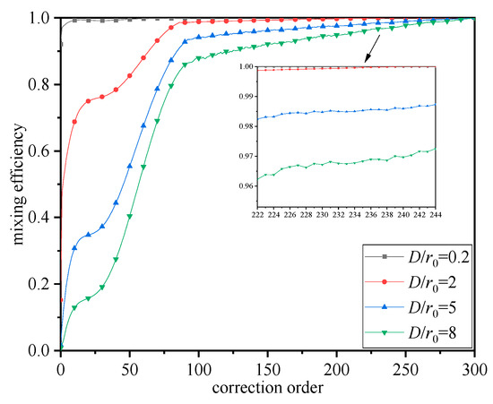
Figure 8.
Relationship between wavefront correction and mixing efficiency in homodyne detection.
Figure 8 shows that when D/r0 is 0.2, the wavefront correction is the same as that under heterodyne detection, and only the correction of 5th-order mixing efficiency converges to 1. When D/r0 is 2, the correction of the 87th-order mixing efficiency is required to reach the extreme value. When D/r0 is 5, the correction of the mixing efficiency below order 234 reaches the extreme value. When D/r0 is 8, it needs to correct the mixing efficiency below order 269 to converge to 1. It is concluded that the effect of the low-order wavefront correction on the mixing efficiency of the system receiving end in homodyne detection is the same as that in heterodyne detection. This is because the integral cosine term of the wavefront phase difference between the signal light and local oscillator light is much larger than the integral sine term, and the influence of low-order wavefront distortion on the mixing efficiency integral sine term is negligible.
Combining Figure 7 and Figure 8, we find that under the influence of atmospheric turbulence, the wavefront correction order required for homodyne detection to reach the wavefront distortion correction limit is higher than that required for heterodyne detection, owing to the higher requirement for spatial phase matching.
According to the trend of wavefront distortion correction with mixing efficiency, we found that when the atmospheric coherence length r0 is certain and the correction of wavefront distortion is of a specific order, there exists a theoretically optimal receiving aperture D that maximizes the mixing gain. Under the conditions of a wavelength of λ = 1550 nm, the signal optical power of Ps = 0.36 μW, local oscillation optical power of Pl = 0.36 mW, and atmospheric coherence length of r0 = 0.05 m, the mixing gain in heterodyne detection and homodyne detection calculated in Equation (14) can be obtained via simulation when the wavefront correction order N in Equation (15) varied. Among them, the simulation results of the curve mixing gain changing with the receiving aperture D in different detection methods are shown in Figure 9, and the optimal mixing gain results are shown in Figure 10.
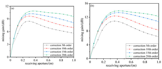
Figure 9.
When the order of wavefront correction is different, the mixing gain varies with the receiving aperture: (a) heterodyne detection; (b) homodyne detection.
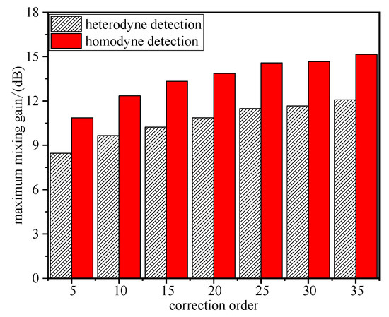
Figure 10.
Variation of wavefront correction order and optimal mixing gain at r0 = 0.05 m.
Figure 9 shows that as the order of wavefront correction increases, the mixing gain increases gradually; and as the receiving aperture D increases, the mixing gain reaches the maximum, and then shows a downward trend. Among them, comparing Figure 9a,b, it is found that the mixing gain obtained by homodyne detection is greater than that obtained by heterodyne detection because the detection sensitivity of homodyne detection itself is better than that of heterodyne detection.
Observing Figure 10 shows that when the D/r0 ratio is 7.6, the best heterodyne detection mixing gain is 8.5 dB, and the best homodyne detection mixing gain is 11.2 dB when correcting the wavefront distortion of the first five orders; the best heterodyne detection mixing gain is 10.3 dB and the best homodyne detection mixing gain is 13.3 dB when correcting the wavefront distortion of the first 15 orders. The mixing gain increase with the wavefront correction order. When the wavefront distortion correction is below the 35th order, the maximum heterodyne detection mixing gain rises to 12.1 dB, and the maximum homodyne detection mixing gain rises to 15.1 dB. The homodyne detection mixing gain is higher than the heterodyne detection mixing gain of about 3 dB.
When considering different detection methods, the same simulation parameters as those in Figure 9 were selected, and under the condition of atmospheric coherence length r0 = 0.01 m, the curves of the mixing gain changing with the receiving aperture D in heterodyne detection and homodyne detection are shown in Figure 11, and the optimal mixing gain results are shown in Figure 12.

Figure 11.
When the order of wavefront correction is different, the mixing gain varies with the receiving aperture: (a) heterodyne detection; (b) homodyne detection.
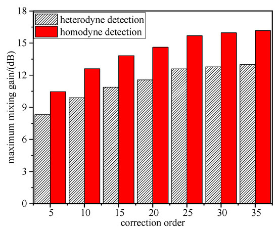
Figure 12.
Variation of wavefront correction order and optimal mixing gain at r0 = 0.01 m.
Figure 11 shows that as the order of wavefront correction increases, the mixing gain increases gradually; and as the receiving aperture D increases, the mixing gain reaches the maximum, and then the mixing gain showed an oscillation decrease. The oscillation mainly comes from the fact that with the increase of turbulence intensity, the energy of the main lobe of the wavefront distortion spreads to the side lobes, which leads to the decrease of the matching degree of the optical field at the receiving end and thus the oscillation phenomenon.
Figure 12 shows that the mixing gain increased as the wavefront correction order gradually increased. In correcting the first five orders of wavefront distortion, the best heterodyne detection mixing gain was 8.3 dB, and the best homodyne detection mixing gain was 11.1 dB. When the wavefront distortion was corrected to below 35 orders, the maximum heterodyne detection mixing gain increased to 12.5 dB, and the maximum homodyne detection mixing gain rose to 15.5 dB. The mixing gain of heterodyne and homodyne detection was optimal when the D/r0 ratio was 11.5. We find that the optimal mixing gain in homodyne detection was generally higher than that in heterodyne detection by approximately 3 dB.
Combining the simulation results of receiving aperture D and mixing gain under different turbulence conditions, it is concluded that as the turbulence intensity increases, the mixing gain is more sensitive to the selection of the receiving aperture. Under a specific turbulence intensity, different orders of wavefront distortion correction will have a suitable receiving aperture to maximize the mixing gain, which provides a quantitative reference for the selection of an optical system in practice.
4. Experiment Research
Through numerical analysis, we found that the effect of low-order wavefront distortion on the mixing efficiency of the coherent detection system was much greater than that of high-order wavefront distortion. To further verify the correctness of the theoretical analysis, the laboratory conducted indoor and outdoor wavefront correction experiments on optical wireless coherent communication systems. The experimental principle is shown in Figure 13. The main experimental equipment is NKT Photonics 1550 nm narrow linewidth laser, a Shack–Hartmann wavefront sensor Imagine Optics Haso4 NIR suitable for 1550 nm, and the deformable mirror was a Thorlabs 40-cell piezoelectric deformable mirror (DM 40) for reduced device complexity. The signal beam is transmitted to the receiver through the receiving antenna and reflected by the piezoelectric deformable mirror through the beam-splitting prism as a parallel outgoing beam. The beam entered the wavefront correction system and was first scaled down by the 4F system to match the photosensitive surface dimensions of the wavefront sensor. A computer-controlled piezoelectric deformable mirror corrected the closed loop for wavefront distortion. The calibrated beam is transmitted into the coupling lens in a parallel optical axis direction and mixed with the local oscillation laser in the experimental control box. The mixer is a Kylia COH24 series mixer, and then the beam was passed through the BPDV2150R balanced detector to view the IF signal through an oscilloscope.
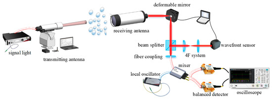
Figure 13.
Schematic diagram of wavefront correction optical wireless coherent communication system.
Based on the wavefront correction principle diagram of the optical wireless coherent communication system, we have built an indoor experiment, as shown in Figure 14. In the indoor experiment, we used the liquid crystal spatial light modulator (LC-SLM) to simulate the wavefront distortion under the disturbance of atmospheric turbulence. The signal beam sent by the laser is incident on the LC-SLM in a phase-only working state, so that the LC-SLM performs phase modulation on the signal beam, thereby generating corresponding wavefront distortion. In this experiment, the receiving aperture D = 105 mm, wavelength λ = 1550 nm, the phase screen size is 60 mm, the grid number is 512 × 512, the transmission distance L = 1000 m, and the phase screen when the atmospheric coherence length r0 = 0.052 m is loaded, simulating the wavefront distortion generated by atmospheric turbulence.
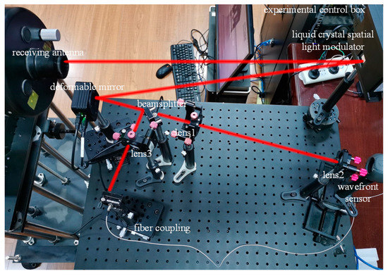
Figure 14.
Physical diagram of indoor experiment.
In the experiment, the D/r0 value was converted to a random corresponding Zernike coefficient of the deformable mirror according to Equation (19), which corresponds to the driving voltage of the deformable mirror. The atmospheric turbulence intensity D/r0 = 2 and the corresponding Zernike coefficients were obtained. The experimental parameters were set as follows: receiving aperture D = 105 mm, wavelength λ = 1550 nm, using integral gain control, integral control coefficient ki = 0.05, and conducting 2000 closed-loop calibration experiments. The wavefront distortion was corrected to the tilt and defocus terms, and the wavefront Zernike coefficients were obtained, as shown in Figure 15.

Figure 15.
Zernike coefficients after wavefront correction.
Figure 15 shows the distribution diagram of Zernike coefficients measured uncorrected, after correction to the tilt item and defocus item in the indoor experiment. It can be seen that when the wavefront correction is not performed, the wavefront coefficients of the tilt and defocus items are larger. The tilt and defocus items account for most of the wavefront distortion, and after using the fully corrected closed-loop control algorithm to correct the tilt and defocus items, respectively, it can be seen that the corresponding low-order wavefront corrected wavefront distortion coefficient is almost 0, and the correction effect of wavefront distortion is good. Moreover, the wavefront distortion of the beam phase is independent and orthogonal in space, and when the wavefront distortion tilt term and defocus term are, respectively, corrected, the remaining orders are not affected.
Figure 16 shows the measured PV and RMS values of the closed-loop wavefront uncorrection and correction. Figure 16 shows that as the number of iterations increases, the PV and RMS values after the closed-loop wavefront correction show a significant downward trend, and after about 500 iterations, the PV and RMS values approach a stable state. Among them, the PV value after correction of the tilt term is stable at 13.2 μm, and the RMS value is stable at 0.81 μm; the PV value after correction of the defocus item is stable at 12.6 μm, and the RMS value is stable at 0.75 μm; the PV value after correction of the astigmatism item is stable at 10.1 μm, and the RMS value is stable at 0.47 μm; we can get that with the increase of the wavefront correction order, the PV and RMS values gradually decrease, and the better the wavefront correction effect.
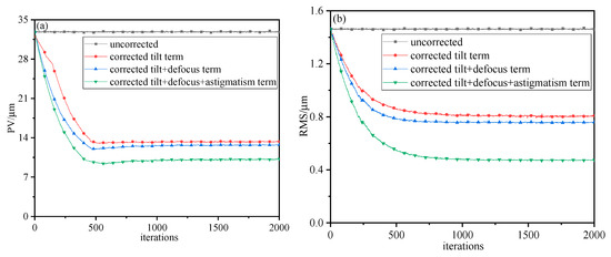
Figure 16.
PV and RMS curves before and after wavefront distortion correction (a) PV curve; (b) RMS curve.
The experimental parameters are set as follows: detector sensitivity R = 0.6 A/W, speed of light c = 2.99 × 10⁸ m/s, quantum efficiency η = 0.8, Planck’s constant h = 6.63 × 10⁻³⁴ J·s, and detector bandwidth B = 40 GHz. Uncorrected and after-corrected the wavefront distortion to the tilt, defocus, and astigmatism terms, the mixing efficiency curves on the receiver side are shown in Figure 17.
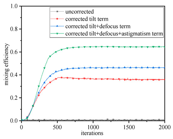
Figure 17.
Relationship between different wavefront corrections and mixing efficiency for D/r0 = 2.
It can be seen from Figure 17 that, comparing the mixing efficiency curve of the coherent detection system at the receiving end uncorrected, the mixing efficiency after correction of different orders of wavefront distortion is significantly improved; among them, in the experimental closed-loop control algorithm with full correction, the mixing efficiency after wavefront correction at a sampling point of 2000, the mixing efficiency after correction of the tilt term is maintained at 36%. Following correction to the defocus them, the mixing efficiency is maintained at 47%. The mixing efficiency is maintained at 62% after correction to the astigmatism term. Following approximately 500 iterations, the mixing efficiency of the system stabilized.
When the experimental environment and parameters were the same as those in Figure 17, the IF signals were acquired under different correction orders. The amplitude changes of the IF signals before and after wavefront correction are shown in Figure 18.
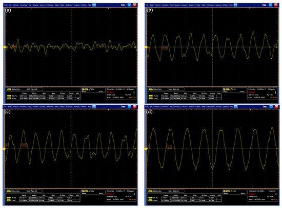
Figure 18.
Amplitude change of the IF signal before and after wavefront correction: (a) uncorrected; (b) corrected tilt term; (c) corrected to defocus term; (d) corrected to astigmatism term.
Figure 18a–d show the waveforms of the IF signal amplitude changes before and after wavefront correction, respectively. In Figure 18a, the IF signal amplitude shows a garbled waveform when it is not corrected, and the peak-to-peak value of the IF signal is only 385.7 mV; In Figure 18b, the IF signal amplitude has a slight fluctuation after the correction of the tilt term only, and the peak-to-peak value of the IF signal is 744.2 mV. In Figure 18c, the waveform changes smoothly after correcting the IF signal amplitude to the defocus term, and the peak-to-peak value of the IF signal is 872 mV. In Figure 18d, the waveform of the IF signal is smooth after the amplitude is corrected to the astigmatism term, and the peak-to-peak of the IF signal is 1.104 V, which benefits the demodulation signal processing at the back end.
According to the experimental system schematic diagram 13, the 1.2 km outdoor experiment was built and data was measured. Figure 19 is a physical map of the outdoor experiment. The main experimental equipment is An NKT Photonics 1550 nm narrow linewidth laser, a Shack–Hartmann wavefront sensor Imagine Optics Haso4 NIR was used, and the deformable mirror was a Thorlabs 40-cell piezoelectric deformable mirror. In the experiment, the laser beam passes through DM 40 and the wavefront sensor to form a closed-loop wavefront correction system. The focal lengths of lens 3 and lens 4 in the 4F beam shrinkage collimation system are 175 mm and 75 mm, respectively. The corrected signal light passes through the beam splitter, is transmitted to the coupling fiber, and undergoes mixing processing. To increase the transmission distance, a reflective link structure is adopted. The transmitting end and the receiving end are both on the 12th floor of Teaching Building No. 6, Jinhua Campus, Xi’an University of Technology, and the reflecting end is on the 8th floor, No. 2 Academic Building, Jinhua Campus, Xi’an University of Technology, the total optical path length is 1.2 km, and there is no building in the middle.
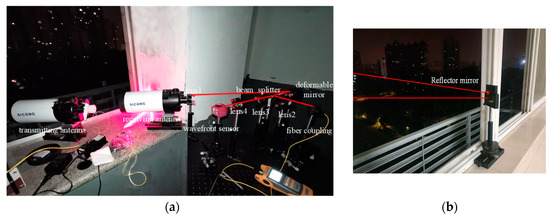
Figure 19.
Physical map of the outdoor experiment: (a) transmitting/receiving end (b) relay end.
The experimental parameters are set as follows: transmission distance L = 1.2 km, receiving aperture D = 105 mm, wavelength λ = 1550 nm, detector sensitivity R = 0.6 A/W, speed of light c = 2.99 × 10⁸ m/s, quantum efficiency η = 0.8, Planck’s constant h = 6.63 × 10⁻³⁴ J·s, detector bandwidth B = 40 GHz, and atmospheric coherence length r0 = 0.055 m. Using integral gain control, the integral control coefficient ki = 0.05 and conducts 2000 closed-loop calibration experiments. The Zernike coefficient changes in Figure 20, the PV and RMS curves are in Figure 21, and the mixing efficiency change curve in Figure 22 shows uncorrected and wavefront correction in the closed-loop state, respectively.
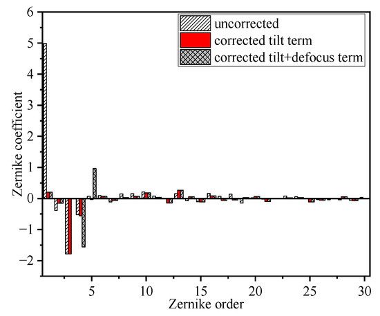
Figure 20.
Zernike coefficients after wavefront correction at 1.2 km.
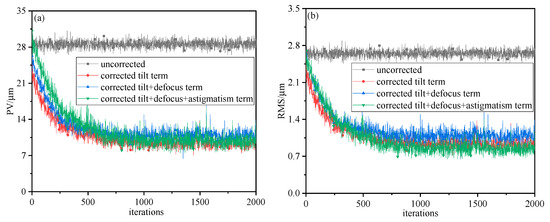
Figure 21.
PV and RMS curves before and after wavefront distortion correction: (a) PV curve; (b) RMS curve.
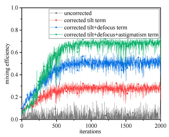
Figure 22.
Relationship between different wavefront corrections and mixing efficiency at 1.2 km.
Figure 20 shows the distribution diagram of Zernike coefficients measured uncorrected and after-correction to the tilt item and defocus item in the outdoor experiment. It can be seen that when the wavefront correction is not performed, the wavefront coefficients of the tilt and defocus items are larger. The tilt and defocus items account for most of the wavefront distortion after using the fully corrected closed-loop control algorithm to correct the tilt and defocus items, respectively. It can be seen that the wavefront distortion coefficient after correction corresponding to the low-order wavefront attenuates significantly. Compared with the indoor experimental results, the correction effect is affected by the unstable factors of the external field environment, so the effect is not as good as the indoor experiment.
Figure 21 depicts the PV and RMS values before and after wavefront correction for a transmission distance of 1.2 km. Among them, the uncorrected PV value is about 28.3 μm, and the RMS value is about 2.7 μm. The PV value and RMS value after correction of different orders of wavefront distortion drop significantly. We can get that with the increase of the wavefront correction order, the PV value and RMS value gradually decrease, and the better the wavefront correction effect.
In the outdoor experiment, Uncorrected and after-corrected wavefront distortion to the tilt, defocus, and astigmatism terms, and the mixing efficiency curve on the receiver side is shown in Figure 22.
As shown in Figure 22, comparing the mixing efficiency curve of the coherent detec-tion system at the receiving end uncorrected, the mixing efficiency after correction of different orders of wavefront distortion is significantly improved; among them, in the experimental closed-loop control algorithm with full correction, the mixing efficiency after correction of the tilt term is maintained at 36%; following correction to defocus them, the mixing efficiency is maintained at 51%, and the mixing efficiency is maintained at 68% after correction to the astigmatism term. Following approximately 500 iterations, the mixing efficiency of the system stabilized.
5. Discussion
For suppressing atmospheric turbulence, reducing the attenuation of signal light, and improving the performance of the optical wireless coherent detection system, further optimization includes the following aspects: First, to correct the random change of the polarization state of the signal light caused by atmospheric turbulence, our laboratory designed a small step back-reset algorithm for polarization control in terms of the polarization state of the beam. The experimental results show that the polarization control system measured at a communication distance of 1.3 km can reduce the variance of signal light fluctuations to an order of magnitude of 10−3, and the mixing efficiency at the receiving end has increased by about 64%; Second, the adaptive optics technology is applied to the multiple-input multiple-output (MIMO) system, and the wavefront correction of the beam-combining received signal can effectively suppress the wavefront distortion, thereby further improving the mixing efficiency of the coherent detection system; Finally, combining the metalens with a coherent receiver, the metalens can effectively reduce the angle of arrival jitter caused by atmospheric turbulence [33], and applying it to a coherent receiver can further improve the mixing efficiency at the receiving end and improve the performance of the coherent detection system.
Based on existing research, combined with the performance limit of the optical wireless coherent detection system, the correction order of wavefront distortion is analyzed, and for the optimal receiving aperture D, the mixing gain is maximized. In addition, to improve the performance of the coherent detection system at the receiving end, multi-beam transmission at the receiving end can be used, combined with the method in this paper, to determine the optimal wavefront correction order and optimal receiving aperture for the coherent detection system, and to further achieve optimal coherent detection. These research programs can be combined to provide help for further correcting the effect of atmospheric turbulence and improving the performance of the optical wireless coherent detection system. Next, it is our ongoing work to study the performance improvement of coherent detection systems by multi-beam delivery in different turbulence models.
6. Conclusions
This study proposed the mode expansion effect of wavefront distortion caused by atmospheric turbulence on the performance of coherent detection systems and the improvement limits for the mixing efficiency, and mixing gain at the receiving end. The effect of wavefront distortions of different orders on the performance of coherent detection systems was verified through experiments. The results are as follows: The mixing efficiency decreased rapidly in a small range of wavefront distortion amplitudes and then decayed regularly. Moreover, the wavefront correction orders required for homodyne detection were larger than those required for heterodyne detection for both detection methods, converging to the extreme value of the mixing efficiency. We also determined the best distortion correction for wavefront distortion that could be provided within the limits of the receiver aperture size. The best mixing gain obtained for homodyne detection was approximately 3 dB larger than that for heterodyne detection. Finally, a coherent detection system experiment verification based on wavefront distortion and its correction was conducted. The indoor experimental results show that when the number of sampling points is 2000, the mixing efficiency after wavefront correction to tilt, defocus, and astigmatism terms is maintained at 36%, 47%, and 62%, respectively; the outdoor experimental results show that when the number of sampling points is 2000, the mixing efficiency after wavefront correction to tilt, defocus, and astigmatism terms is maintained at 36%, 51%, and 68%,respectively, consistent with the numerical simulation results.
Therefore, in the actual wavefront distortion correction work of an optical wireless coherent communication system, the mixing gain obtained by using homodyne detection is higher than that obtained by heterodyne detection. However, the required wavefront correction orders are greater than the heterodyne detection wavefront correction orders to achieve the best mixing efficiency.
Author Contributions
Conceptualization, X.K.; methodology, X.K., S.Y. and T.X.; software, T.X.; validation, T.X. and J.L.; formal analysis, C.K.; investigation, S.Y.; resources, S.Y. and T.X.; data curation, S.Y. and T.X.; writing—original draft preparation, S.Y. and T.X.; writing—review and editing, S.Y. and J.L. All authors have read and agreed to the published version of the manuscript.
Funding
The Key Industrial Innovation Chain Project of Shaanxi Province [grant number 2017ZDCXLGY-06-01, 2020ZDLGY05-02]; the Xi’an Science and Technology Planning Project [grant number 2020KJRC0083]; the Scientific Research Plan Projects of Shaanxi Education Department (18JK0341); and the Xi’an Science and Technology Plan (22GXFW0115).
Institutional Review Board Statement
Not applicable.
Informed Consent Statement
Not applicable.
Data Availability Statement
The data that support the findings of this study are available from the corresponding author upon reasonable request.
Conflicts of Interest
The authors declare no conflict of interest.
References
- Liu, Y.J.; Chen, K.; Song, S.; Pan, Y.; Liu, Y.C.; Guo, L. Reinforcement learning aided geometric shaping and self-canceling coherent detection for a PAM4 FSO communication system. J. Opt. Commun. Netw. 2022, 15, 16–28. [Google Scholar] [CrossRef]
- Wang, Y.Y.; Liu, W.C.; Zhou, X.Y. Splitting Receiver With Joint Envelope and Coherent Detection. IEEE Commun. Lett. 2022, 26, 1328–1332. [Google Scholar] [CrossRef]
- Liu, Y.T.; Gao, M.D.; Zeng, X.D.; Liu, F.; Bi, W.H. Factors influencing the applications of active heterodyne detection. Opt. Lasers Eng. 2021, 146, 106694. [Google Scholar] [CrossRef]
- Suleiman, I.; Nielsen, J.A.H.; Guo, X.; Jain, N.; Neergaard-Nielsen, J.; Gehring, T.; Andersen, U.L. 40 km Fiber Transmission of Squeezed Light Measured with a Real Local Oscillator. Quantum Phys. 2022, 7, 1328–1332. [Google Scholar] [CrossRef]
- Ke, X.; Wu, J. Wavefront correction system. In Coherent Optical Wireless Communication Principle and Application, 1st ed.; Li, P., Ed.; China Science Publishing & Media Ltd.: Beijing, China, 2019; Volume 6, pp. 225–252. [Google Scholar]
- Banakh, V.A.; Zhmylevskii, V.V.; Ignatiev, A.B.; Morozov, V.V.; Razenkov, I.A.; Rostov, A.P.; Tsvyk, R.S. Optical-beam wavefront control based on the atmospheric backscatter signal. Quantum Electron. 2015, 45, 153–160. [Google Scholar] [CrossRef]
- Hu, L.J.; Hu, S.W.; Gong, W.; Si, K. Learning-based Shack-Hartmann wavefront sensor for high-order aberration detection. Opt. Express 2019, 27, 33504–33517. [Google Scholar] [CrossRef]
- Zhang, Z.T.; Bharmal, N.; Morris, T.; Liang, Y.H. Laboratory quantification of a plenoptic wavefront sensor with extended objects. Mon. Not. R. Astron. Soc. 2020, 497, 4580–4586. [Google Scholar] [CrossRef]
- Rani, N.; Singh, P.; Kaur, P. Mitigation of Scintillation Effects in WDM-FSO System Using Homodyne Detection. Optik 2021, 248, 168165. [Google Scholar] [CrossRef]
- Yan, X.; Cao, C.Q.; Zhang, W.R.; Zeng, X.D.; Feng, Z.J.; Wu, Z.Y.; Wang, T. Wavefront Detection and Compensation Technology Based on Signal Light Nutation under Atmospheric Turbulence. IEEE Commun. Lett. 2021, 25, 3340–3344. [Google Scholar] [CrossRef]
- Zhong, Z.Q.; Zhang, X.; Zhang, B.; Yuan, X. Mitigation of atmospheric turbulence effect by light beams carrying self-rotating wavefront. Opt. Express 2022, 30, 24421–24430. [Google Scholar] [CrossRef]
- Betanzos-Torres, M.A.; Castillo-Mixcóatl, J.; Muoz-Aguirre, S.; Beltrán-Pérez, G. Adaptive optics system simulator—ScienceDirect. Opt. Laser Technol. 2018, 105, 118–128. [Google Scholar] [CrossRef]
- Lechner, D.; Zepp, A.; Eichhorn, M.; Gladysz, S. Adaptable Shack-Hartmann wavefront sensor with diffractive lenslet arrays to mitigate the effects of scintillation. Opt. Express 2020, 28, 36188–36205. [Google Scholar] [CrossRef] [PubMed]
- Zhang, M.; Jiang, L.; Huang, Z. Adaptive optics technology and urban horizontal link laser communication system. Opt. Eng. 2018, 60, 116107. [Google Scholar] [CrossRef]
- Norris, B.R.M.; Wei, J.; Betters, C.H.; Wong, A.; Leon-Saval, S.G. An all-photonic focal-plane wavefront sensor. Nat. Commun. 2020, 11, 5335. [Google Scholar] [CrossRef] [PubMed]
- Quintavalla, M.; Bergomi, M.; Magrin, D.; Bonora, S.; Ragazzoni, R. Correction of non-common path aberrations in pyramid wavefront sensors to recover the optimal magnitude gain using a deformable lens. Appl. Opt. 2020, 59, 5151–5157. [Google Scholar] [CrossRef]
- Yang, Y.F.; Yan, C.X.; Hu, C.H.; Wu, C.J. Modified heterodyne efficiency for coherent laser communication in the presence of polarization aberrations. Opt. Express 2017, 25, 7567–7591. [Google Scholar] [CrossRef]
- Stotts, L.B.; Andrews, L.C. Adaptive optics model characterizing turbulence mitigation for free space optical communications link budgets. Opt. Express 2021, 29, 20307–20321. [Google Scholar] [CrossRef]
- Hu, L.J.; Hu, S.W.; Li, Y.N.; Gong, W.; Si, K. Reliability of wavefront shaping based on coherent optical adaptive technique in deep tissue focusing. J. Biophotonics 2021, 13, e201900245. [Google Scholar] [CrossRef]
- Wu, J.L.; Ke, X.Z.; Yang, Y.Q.; Liang, J.Y.; Liu, M.Y. Correction of Distorted Wavefront Using Dual Liquid Crystal Spatial Light Modulators. Photonics 2022, 9, 426. [Google Scholar] [CrossRef]
- Xu, D.L.; Yue, P.; Yi, X. A Theoretical Analysis Method of OAM-Based FSO Error Performance. Acta Electron. Sin. 2021, 49, 1934–1944. [Google Scholar]
- Liu, Q.; Chew, K.-H.; Huang, Y.; Liu, C.; Hu, X.; Li, Y.; Chen, R.-P. Effect of Twisting Phases on the Polarization Dynamics of a Vector Optical Field. Photonics 2022, 9, 722. [Google Scholar] [CrossRef]
- Ren, J.Y.; Sun, H.Y.; Zhang, L.X.; Zhao, Y.Z. Receiving characteristics analysis of large dynamic range based on four-optic coherent mixing. Optik 2020, 221, 165348. [Google Scholar] [CrossRef]
- Karar, A.S.; Falou, A.R.E.; Barakat, J.M.H.; Gürkan, Z.N.; Zhong, K. Recent Advances in Coherent Optical Communications for Short-Reach: Phase Retrieval Methods. Photonics 2023, 10, 308. [Google Scholar] [CrossRef]
- Magidi, S.; Jabeena, A. Free Space Optics, Channel Models and Hybrid Modulation Schemes: A Review. Wirel. Pers. Commun. 2021, 119, 2951–2974. [Google Scholar] [CrossRef]
- Fice, M.J.; Chiuchiarelli, A.; Ciaramella, E.; Seeds, A.J. Homodyne coherent optical receiver using an optical injection phase-lock loop. J. Light. Technol. 2011, 29, 1152–1164. [Google Scholar] [CrossRef]
- Liu, C.; Chen, S.; Li, X.Y.; Xian, H. Performance evaluation of adaptive optics for atmospheric coherent laser communications. Opt. Express 2014, 22, 15554–15563. [Google Scholar] [CrossRef]
- Geng, C.; Li, F.; Zuo, J.; Liu, J.Y.; Yang, X.; Yu, T.; Jiang, J.L.; Li, X.Y. Fiber laser transceiving and wavefront aberration mitigation with adaptive distributed aperture array for free-space optical communications. Opt. Lett. 2020, 45, 1906–1909. [Google Scholar] [CrossRef]
- Konwar, S.; Boruah, B.R. Leveraging the orthogonality of Zernike modes for robust free-space optical communication. Commun. Phys. 2020, 3, 203. [Google Scholar] [CrossRef]
- Erol, B.; Altiner, B.; Adali, E.; Delibasi, A. H-infinity Suboptimal controller design for adaptive optic systems. Trans. Inst. Meas. Control. 2019, 41, 2100–2113. [Google Scholar] [CrossRef]
- Paneva-Konovska, J. A family of hyper-Bessel functions and convergent series in them. Fract. Calc. Appl. Anal. 2014, 17, 1001–1015. [Google Scholar] [CrossRef]
- Soto-Quiros, P.; Torokhti, A. Optimal transforms of random vectors: The case of successive optimizations. Signal Process. 2017, 132, 183–196. [Google Scholar] [CrossRef]
- Im, C.S.; Lee, W.B.; Gwon, J.Y.; Lee, S.S. Float optical phased array receiver incorporating an on-chip metalens concentrator. Opt. Lett. 2022, 47, 2060–2063. [Google Scholar] [CrossRef] [PubMed]


Disclaimer/Publisher’s Note: The statements, opinions and data contained in all publications are solely those of the individual author(s) and contributor(s) and not of MDPI and/or the editor(s). MDPI and/or the editor(s) disclaim responsibility for any injury to people or property resulting from any ideas, methods, instructions or products referred to in the content. |
© 2023 by the authors. Licensee MDPI, Basel, Switzerland. This article is an open access article distributed under the terms and conditions of the Creative Commons Attribution (CC BY) license (https://creativecommons.org/licenses/by/4.0/).