Bionic Compass Method Based on Atmospheric Polarization Optimization in Non-Ideal Clear Condition

Abstract

The bionic polarization compass is a fascinating subject in the navigation domain. Existing polarization navigation models are primarily based on Rayleigh scattering theory, which is applicable to high-altitude, dry, and clear weather conditions. In most scenarios, it is difficult to meet such ideal clear conditions. This paper proposes a bionic navigation method based on atmospheric polarization optimization to improve heading accuracy under non-ideal clear conditions. A signal model under non-ideal clear conditions was firstly established to introduce disturbances of aerosols and other particles into the raw signal function acquired by a camera. Then, an energy functional optimization model was constructed to eliminate the disturbances caused by large particle scattering and restore the original sky polarization pattern. Subsequently, the heading angle was calculated using astronomical data, enhancing accuracy under non-ideal conditions. Finally, we constructed a polarization compass system and conducted field experiments. The results demonstrate that the proposed algorithm effectively mitigates the impact of scattering from aerosols and other particles, reducing the heading angle error to within 2° under sunny, cloudy, overcast and sandy conditions.

1. Introduction

Under clear skies, Rayleigh scattering causes the atmospheric polarization pattern to change in a stable and predictable manner with the position of the sun [1]. Polarization navigation utilizes this pattern as a signal source to determine the carrier’s directional information by detecting and analyzing the atmospheric polarization distribution [2]. This method offers advantages such as full autonomy, strong resistance to interference, and measurement errors that do not accumulate over time, making it an effective complement to existing navigation technologies.

There are two main approaches to detecting sky polarization patterns: point-source detection and camera imaging detection [3]. Point-source measurements involve the measurement of polarization patterns at one or a few points in the sky [4]; camera imaging measurements enable the acquisition of polarization patterns across the entire sky region [5]. Currently, imaging sensors are commonly used to extract directional information for polarization navigation. Based on this approach, researchers have proposed various heading calculation methods. The least-squares method has been employed to fit the solar meridian for localization purposes [6,7]. Polarization information from the zenith has been detected and used as a compass to calculate the heading angle [8,9,10,11,12]. A symmetry analysis method for orientation was developed by extracting the symmetry of polarization patterns [13,14,15]. Furthermore, an angle algorithm based on the polarization electric field vectors perpendicular to the solar direction vector has been proposed to determine heading [16,17].

Although polarization navigation provides real-time absolute orientation with simple computation and no cumulative errors, its accuracy is highly dependent on weather conditions and air quality. The ideal observation scenario for polarization navigation is under high-altitude, dry, and clear conditions. In non-ideal conditions, such as cloudy or sandy conditions, scattering by aerosols, cloud droplets, and dust particles disrupts the polarization pattern, leading to errors in the derived polarization information. These errors propagate through polarization orientation models, ultimately reducing heading accuracy [18]. Therefore, further research is needed to address polarization orientation challenges under non-ideal conditions. Tang et al. applied a spiking neural network to filter polarization images and combined it with the least squares method to achieve orientation under non-ideal conditions [19]. Wu et al. used the principal component analysis network to extract polarization image features under various weather conditions and improved the trilateral weighted sparse coding algorithm to eliminate noise in atmospheric polarization images [20]. Li et al. proposed a gradient-based segmentation method for polarization degree images and developed a convolution-based in-region drawing algorithm to correct the navigation errors caused by blurring [21]. Zhang et al. employed an improved U-Net deep neural network combined with a polarization degree threshold to perform cloud segmentation, removing anomalous pixels in polarization azimuth images corresponding to cloudy areas [22]. Pu et al. utilized a generative adversarial network model to reconstruct sky polarization patterns under adverse weather conditions, addressing random disturbances caused by weather and geographical environments [23]. Li et al. simulated a light transport model using the Monte Carlo method to derive the macroscopic optical properties of clouds and calculated the polarization influence factors of the clouds [24]. Their experiments demonstrated that the “depolarization effect” of particles such as water clouds is weakest in the ultraviolet (UV) band. Wang et al. developed an ultraviolet–visible bionic light compass system, incorporating the ultraviolet band into polarization detection and reframing navigation under cloudy conditions as a multi-classification problem to mitigate the interference caused by cloud scattering [17].

The aforementioned methods enable polarization orientation under non-ideal conditions, such as cloudy skies, but they still have certain limitations. Neural-network-based approaches for filtering and reconstructing polarization patterns require substantial time and large datasets for training [2]. However, due to constraints such as weather conditions, geographical environments, and equipment limitations, obtaining large datasets for network training is challenging in real-world scenarios [23]. The UV band can partially counteract the “depolarization effect” caused by large particle scattering. Nevertheless, polarization orientation devices based on UV detection require multiple UV cameras to operate simultaneously [18], resulting in complex structures and high costs. Therefore, an easy-to-deploy and simple algorithm is needed to meet the demands of polarization navigation under non-ideal conditions. This paper proposes a bionic navigation method based on atmospheric polarization optimization to investigate a polarization signal model and heading calculation mechanism under non-ideal clear conditions. First, the disturbances from large particles such as dust are incorporated into the raw signal captured by the camera, establishing a signal transmission model for non-ideal conditions. Subsequently, an energy generalized optimization model is constructed for optimization on the basis of the signal function with disturbances attached. This optimization model is solved by the dual exact minimization method to eliminate the errors caused by large particle scattering and restore the original sky polarization pattern. Then, combined with an astronomical calendar, the heading angle is solved to realize the purpose of navigation. To verify this method, a bionic polarization compass system was constructed for field experiments. The experimental results highlight that the proposed algorithm remained robust under sunny weather conditions with clouds and dust, proving to be a viable option.

This article is organized as follows. Section 2 presents the establishment and simulation of the atmospheric polarization pattern. Section 3 describes the polarization optimization model and the heading angle acquisition algorithm. The experimental system and results are given in Section 4. We finally draw conclusions and perspectives of this work in Section 5.

2. Formation of the Skylight Polarization Field

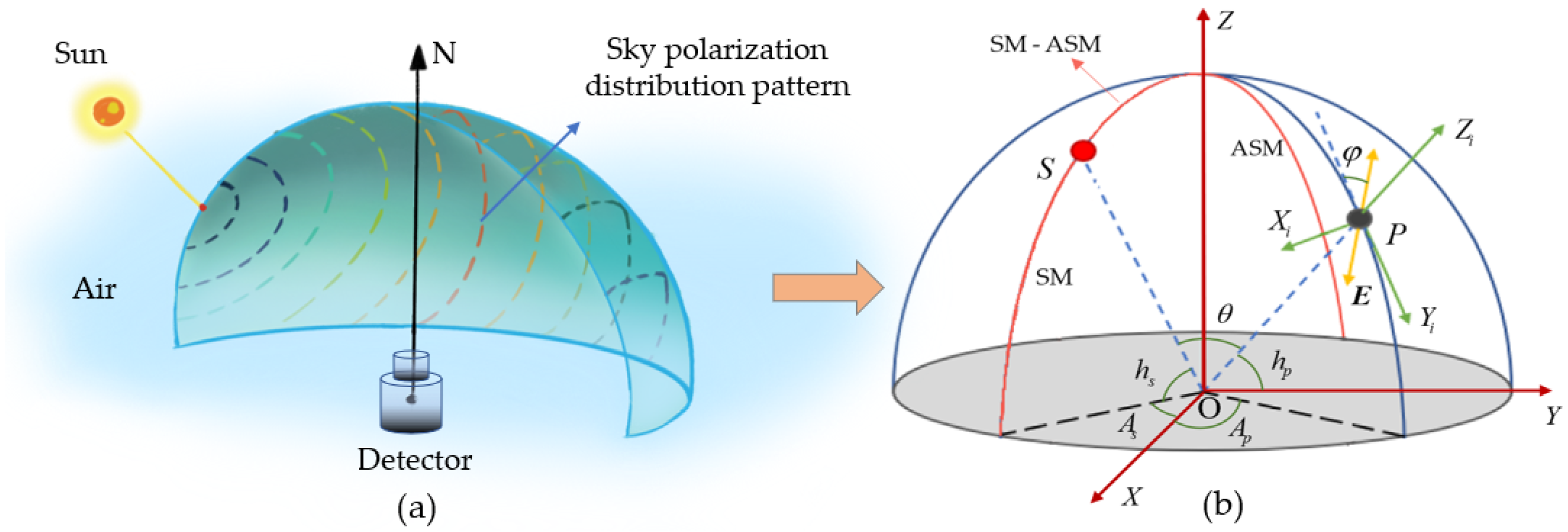
The concept of biomimetic polarized light detection is illustrated in Figure 1. Sunlight is unpolarized; however, before it reaches the Earth’s surface, it undergoes refraction or scattering owing to various particles in the atmosphere. Consequently, the incident sunlight becomes polarized, thereby resulting in a skylight polarization distribution pattern. The establishment of an atmospheric polarization model is based on the entire sky. To facilitate calculations, a celestial coordinate system is created, as shown in Figure 1b. The coordinate origin $O$ represents the position of the detector (i.e., the observer), while $OXYZ$ represents the geographic coordinate system. $S$ denotes the position of the sun, $P$ represents the position of the observed point in the sky, and $N$ indicates the zenith. The solar meridian (SM) is the arc that connects the sun to the zenith, and its extension in the opposite direction is called the anti-solar meridian (ASM). $P{X}_i{Y}_i{Z}_i$ is the local coordinate frame of a scattering point. $\mathit{E}$ and $\phi$ are the electric vector vibration direction and the angle of polarization (AOP) at point $P$, and $\theta$ is the scattering angle.

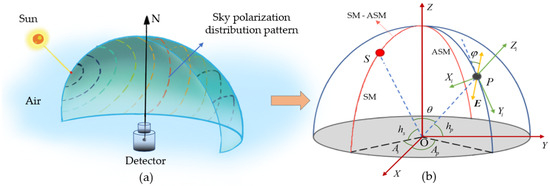
Figure 1. Illustration of the sky polarization mode detection process. (a) Formation schematic of the sky’s polarization distribution pattern; (b) a mathematical model for polarization mode detection.

Assuming that the radius of the celestial sphere is 1, $\mathit{O}\mathit{S}$ and $\mathit{O}\mathit{P}$ can be calculated according to Figure 1b

$$\mathit{O}\mathit{S}=\cos h_s\cos A_s\mathit{x}+\cos h_s\sin A_s\mathit{y}+\sin h_s\mathit{z}$$

(1)

$$\mathit{O}\mathit{P}=\cos h_p\cos A_p\mathit{x}+\cos h_p\sin A_p\mathit{y}+\sin h_p\mathit{z}$$

(2)

where $\mathit{x}$, $\mathit{y}$ and $\mathit{z}$ are the unit vectors along the $X$, $Y$ and $Z$ coordinate axes, respectively; $h_s$ represents the solar altitude angle; and $A_s$ denotes the solar azimuth angle. Correspondingly, $h_p$ and $A_p$ represent the elevation and azimuth angles of the observed point $P$. The cosine of the scattering angle $\theta$ can be calculated using Equation (3):

$$\begin{array}{ccc}\hfill \cos \theta & \hfill =\hfill & \mathit{O}\mathit{S}\cdot \mathit{O}\mathit{P}\hfill \\ & \hfill =\hfill & \sin h_s\sin h_p+\cos h_s\cos h_p\cos (A_p-A_s)\hfill \end{array}$$

(3)

According to Rayleigh scattering theory, the degree of polarization (DOP) and the angle of polarization (AOP) of $P$ can be represented by Equations (4) and (5) [18].

$$P(\theta )={\displaystyle \frac{{\sin }^2(\theta )}{1+{\cos }^2(\theta )}}$$

(4)

$$\tan \phi ={\displaystyle \frac{\sin h_s\cos h_p-\cos h_s\sin h_p\cos (A_p-A_s)}{-\cos h_s\sin (A_p-A_s)}}$$

(5)

According to the above Equations (4) and (5), the DOP and AOP at point $P$ can be determined. Similarly, the polarization information for other observed points throughout the sky can be obtained using the same method. Then, a three-dimensional model of the skylight polarization field based on Rayleigh scattering can be established, as shown in Figure 2.

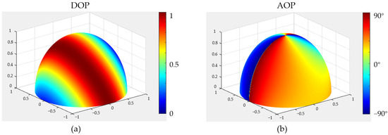
Figure 2. Three-dimensional simulation of skylight polarization field, (a) DOP and (b) AOP.

3. Bionic Navigation Algorithm Based on Atmospheric Polarization Optimization

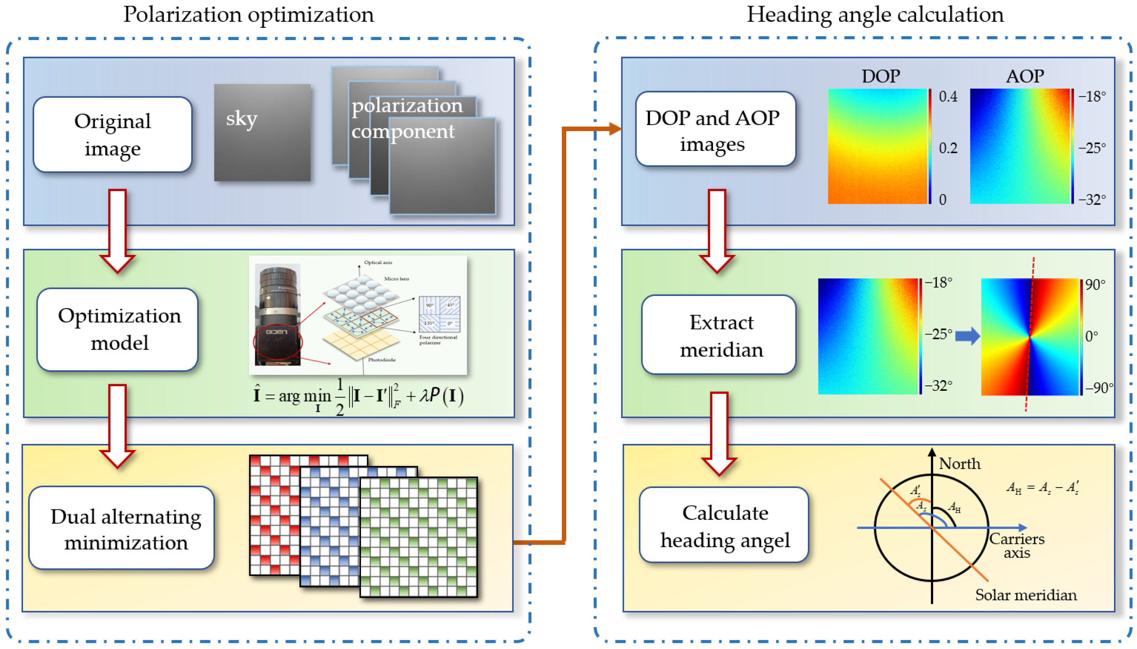
The process of the heading determination algorithm is shown in Figure 3. It is mainly divided into two parts: polarization optimization model and heading angle calculation. The polarization optimization model is used to optimize the original polarization image acquired by the camera and filter out the disturbance terms brought by the scattering of aerosols and other particles. Then, the optimized polarization image is used to calculate the skylight polarization pattern, and the heading angle is calculated by combining the results with astronomical data, thereby achieving accurate heading determination.

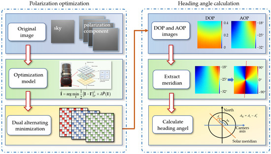
Figure 3. Process of heading determination algorithm.

3.1. Optimization Model Based on the Atmospheric Polarization Energy Functional

Rayleigh scattering describes the phenomenon where particles with a radius much smaller than the wavelength of the incident light scatter the incoming light. For atmospheric polarization models based on Rayleigh scattering, ideal observation conditions are high-altitude, dry, and clear skies. However, in practice, most observation sites struggle to meet these ideal criteria. Under non-ideal circumstances such as partially cloudy, overcast, or sandy conditions, the atmosphere may contain not only gaseous molecules but also aerosols, cloud droplets, and dust particles. In such cases, the polarization distribution of the sky, based solely on Rayleigh scattering, is affected by the multiple scattering caused by these additional particles.

Given the discrepancies between measured polarization data and theoretical polarization models, directly using the polarization patterns obtained from cameras makes it challenging to achieve high-precision orientation under non-ideal clear weather conditions. Therefore, it is essential to process these data to minimize such errors as much as possible.

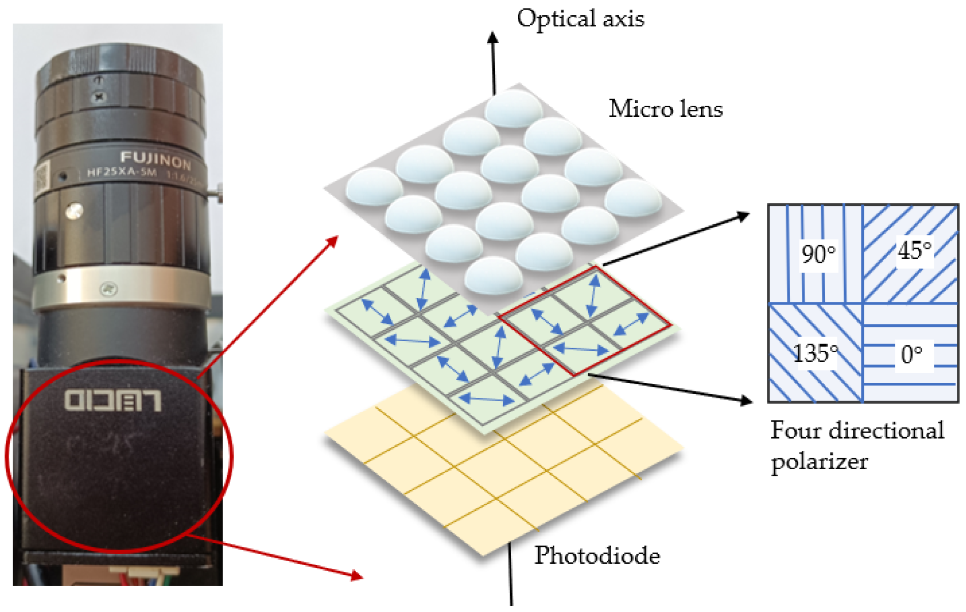
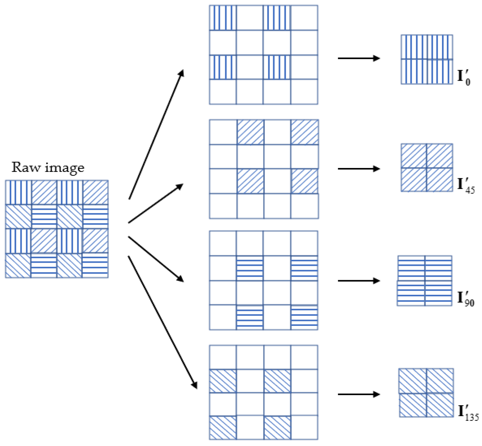
The experimental camera used in this study was the PHX050S-P polarization light camera (LUCID, Canada). This camera is composed of a micro lens, four-directional polarizer, and photodiode array, as shown in Figure 4. The four-directional polarizer enables the camera to take a four-directional polarization (0°, 45°, 90°, and 135°) image in one shot. Based on the distribution of the four-directional polarizer, the raw image captured by the camera can be split into four images ($I_{\mathrm{0}}^{\prime }$, $I_{\mathrm{45}}^{\prime }$, $I_{\mathrm{90}}^{\prime }$ and $I_{\mathrm{135}}^{\prime }$), each corresponding to a different polarization direction, as shown in Figure 5. This method enhances the efficiency of obtaining multi-directional polarization information and reduces the errors caused by multiple shots.

Figure 4. Structure of the polarized light camera.

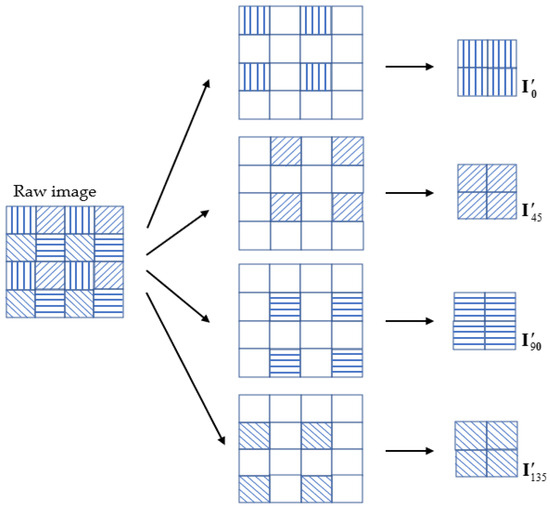
Figure 5. Schematic diagram of raw image splitting.

The intensity sub-image $I^{\prime }$ collected by the camera is a combination of the ideal signal and the interference signals caused by aerosol and water vapor scattering. It can be expressed by Equation (6) [25]:

$$I^{\prime }(x,y)=I(x,y)+N(x,y)$$

(6)

where $I^{\prime }$ represents the noisy original sub-image observed by the camera, $I$ represents the “true” image we aim to restore, $(x,y)$ indicates the position of the pixel in the image, and $N$ represents the interference signal caused by scattering from other particles.

The functional $P$ of $I$ is defined as follows [26], which represents the overall variation in the image:

$$P[{\rm I}(x,y)]={\displaystyle \underset{\Omega }{\iint }\left|\nabla I(x,y)\right|}dxdy$$

(7)

where $\nabla I(x,y)$ represents the gradient field of $I$, $\left|\cdot \right|$ represents the Euclidean norm, and $\Omega$ represents the domain of $I$, i.e., the entire sub-image area, corresponding to the sensor’s sensitive area under this polarization channel.

Treating the distance between each adjacent pixel as a unit length, Equation (7) can be discretized to obtain:

$$P[{\rm I}(x,y)]={\displaystyle \sum _{x=1}^m{\displaystyle \sum _{y=1}^n\sqrt{{\left[I(x,y)-I(x+1,y)\right]}^2+{\left[I(x,y)-I(x,y+1)\right]}^2}}}$$

(8)

where $m$ and $n$ represent the number of rows and columns of the image, respectively.

The value of the functional in image with disturbances is significantly greater than in the image without disturbances [26]. To filter out disturbances, an optimization model can be constructed as shown in Equation (9) to achieve the minimization of the functional [27], thereby recovering the original sky image.

$$\widehat{I}=\arg \underset{I}{\min }\left\{{\displaystyle \frac{1}{2}}{‖I-I^{\prime }‖}_F^2+\lambda P\left(I\right)\right\}$$

(9)

where $1/2{‖I-I^{\prime }‖}_F^2$ represents the data fidelity term, $\lambda P\left(I\right)$ represents the regularization term, $\lambda$ is the regularization parameter, and $\widehat{I}$ represents the optimized intensity signal. The regularization term filters out disturbances by controlling the gradient of the image. The data fidelity term manages the discrepancy between the denoised result and the original image, preventing excessive smoothing. The regularization parameter $\lambda$ controls the balance between smoothness and fidelity to the observed data. This optimization model suppresses small fluctuations caused by the scattering from large particles while preserving the essential features in the image, resulting in a more accurate restoration of the sky image.

In the optimization process, the initial value of $I$ is set to $I^{\prime }$, and $I$ is iteratively updated to minimize Equation (9). By solving this optimization model, errors introduced by scattering from aerosols, water vapor, and other particles can be reduced, resulting in an intensity signal that filters out disturbances.

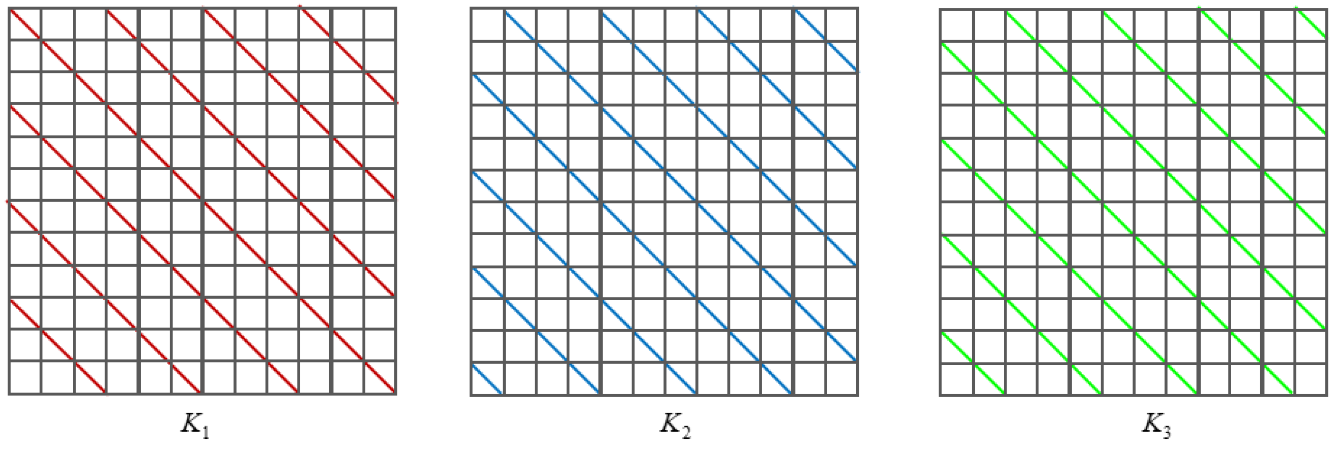
For ease of calculation, Equation (8) is decomposed into separable functions. First, the diagonals of $I$ are divided into three groups, with the division criteria shown in Equation (10), as illustrated in Figure 6.

$$\begin{array}{ccc}\hfill K_i& \hfill \equiv \hfill & \{k\in \{-(m-1),\dots ,n-1\}:(k+1-i)\mathrm{mod}3=0\}\hfill \\ \hfill i& \hfill =\hfill & 1,2,3\hfill \end{array}$$

(10)

where $K_i$ represents the divided diagonal set and $k$ represents the specific diagonal. For $k=0$, $k$ represents the main diagonal; for $k>0$, it represents the diagonal above the main diagonal; and for $k<0$, it represents the diagonal below the main diagonal.

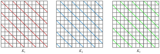
Figure 6. The schematic diagram of diagonal division.

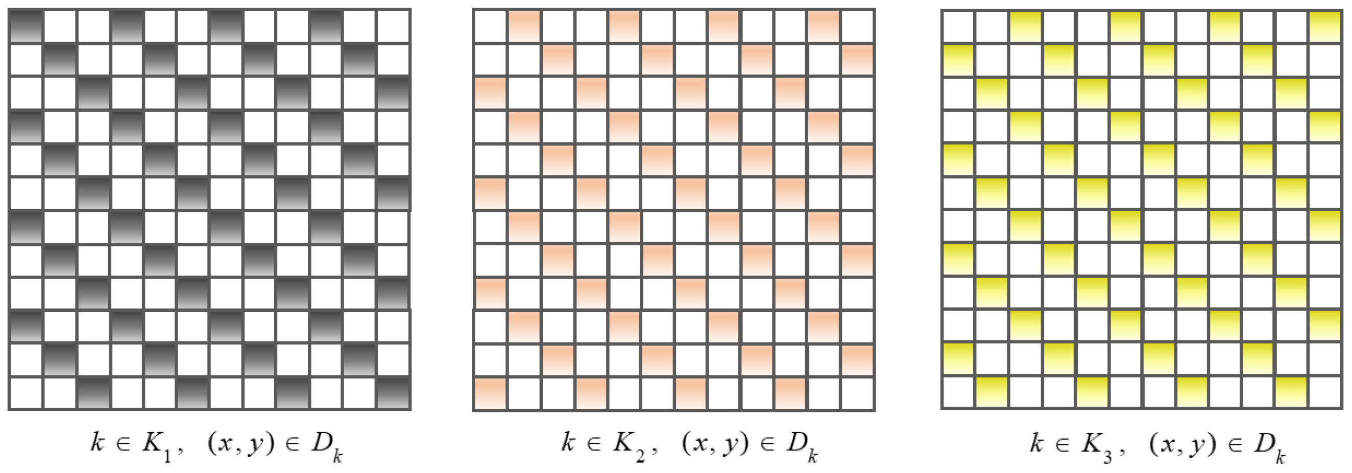
Let $D_k$ represent the set of pixels on the $k$-th diagonal, where $D_0$ denotes the index set of the main diagonal. Based on this diagonal division, the pixel set of $I$ can also be divided into three groups, forming three blocks, as shown in Figure 7.

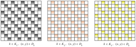
Figure 7. The schematic diagram of pixel division.

This particular partition of the diagonals is the one with the smallest amount of sets such that for any $a,b\in K_i$, we have $|a-b|>2$ to guarantee that the function is separable. Under this division, Equation (8) can be rewritten as:

$$\begin{array}{ccc}\hfill P[{\rm I}(x,y)]& \hfill =\hfill & {\displaystyle \sum _{x=1}^m{\displaystyle \sum _{y=1}^n\sqrt{{\left[I(x,y)-I(x+1,y)\right]}^2+{\left[I(x,y)-I(x,y+1)\right]}^2}}}\hfill \\ & \hfill =\hfill & {\displaystyle \sum _{k\in K_1}{\displaystyle \sum _{(x,y)\in D_k}\sqrt{{\left[I(x,y)-I(x+1,y)\right]}^2+{\left[I(x,y)-I(x,y+1)\right]}^2}}}\hfill \\ & \hfill +\hfill & {\displaystyle \sum _{k\in K_2}{\displaystyle \sum _{(x,y)\in D_k}\sqrt{{\left[I(x,y)-I(x+1,y)\right]}^2+{\left[I(x,y)-I(x,y+1)\right]}^2}}}\hfill \\ & \hfill +\hfill & {\displaystyle \sum _{k\in K_3}{\displaystyle \sum _{(x,y)\in D_k}\sqrt{{\left[I(x,y)-I(x+1,y)\right]}^2+{\left[I(x,y)-I(x,y+1)\right]}^2}}}\hfill \\ & \hfill =\hfill & {\psi }_1(I)+{\psi }_2(I)+{\psi }_3(I)\hfill \end{array}$$

(11)

Equation (9) can be reformulated as the following minimization problem:

$$\underset{I}{\min }\left\{f(I)+\lambda {\displaystyle \sum _{i=1}^3{\psi }_i(I)}\right\}$$

(12)

with

$$f(I)={\displaystyle \frac{1}{2}}{‖I-I^{\prime }‖}_F^2$$

(13)

This minimization problem can be solved using the dual alternating minimization method [28]. The dual problem of Equation (12) is given by

$$\underset{Q}{\max }\left\{-f^{\ast }\left(-{\displaystyle \sum _{j=1}^3{Q}_j}\right)-\lambda {\displaystyle \sum _{j=1}^3{\psi }_j^{\ast }\left(Q_j\right)}\right\}$$

(14)

where $f^{\ast }(\cdot )=\sup \left(⟨\cdot ,I⟩-f(I)\right)$ and ${\psi }_i^{\ast }(\cdot )=\sup \left(⟨\cdot ,I⟩-{\psi }_i(I)\right)$ are the corresponding conjugate functions, $Q$ represents the dual variable of $I$, and $Q_j$ represents the j-th component of $Q$.

Because Slater’s condition is satisfied and the primal problem is bounded below, strong duality holds [29], which means that the optimal solution of the dual problem is the optimal value of the original problem.

Equation (14) in minimization form can be written as

$$\underset{Q}{\min }\left\{F(Q)+\lambda {\displaystyle \sum _{j=1}^3{\mathsf{\Psi }}_j\left(Q_j\right)}\right\}$$

(15)

with

$$F(Q)\equiv f^{\ast }\left(-{\displaystyle \sum _{j=1}^3{Q}_j}\right), {\mathsf{\Psi }}_j\left(Q_j\right)\equiv {\psi }_j^{\ast }\left(Q_j\right)$$

(16)

According to the dual exact minimization step, the new value of $Q$ on the i-th block is [29]

$$Q_i^{\mathrm{new}}\in \underset{Q_i}{argmin}\left\{f^{\ast }\left(-{\displaystyle \sum _{j=1,j\ne i}^m{\overline{Q}}_j-Q_i}\right)+\lambda {\psi }_i^{\ast }\left(Q_i\right)\right\}$$

(17)

where ${\overline{Q}}_j$ represents the current fixed value of $Q_j$ during an iteration of the optimization process.

3.2. Heading Angle Acquisition Algorithm

The intensity sub-images of the four polarization channels can all be optimized using the aforementioned method to filter out disturbances. After optimization, it is necessary to calculate the polarization pattern. Here, we used Stokes vectors to represent the polarization information of the incident light, expressed as Equation (18).

$$\left\{\begin{array}{l}{\mathbf{S}}_0=0.5\left[I_0+I_{45}+I_{90}+I_{135}\right]\hfill \\ {\mathbf{S}}_1=I_0-I_{90}\hfill \\ {\mathbf{S}}_2=I_{45}-I_{135}\hfill \\ {\mathbf{S}}_3=0\hfill \end{array}\right.$$

(18)

where $S$ represents the Stokes vector, ${\mathbf{S}}_0$ represents the total light intensity received by the detector, ${\mathbf{S}}_1$ represents the difference in light intensity between the incident light at 0° and 90°, ${\mathbf{S}}_2$ is the difference in light intensity between the incident light at 45° and 135°, and ${\mathbf{S}}_3$ is the circularly polarized light. Note that the circular polarization component can be ignored in most cases [30].

The DOP and AOP of the incident light can be calculated as follows:

$$\mathrm{DOP}={\displaystyle \frac{\sqrt{{{\mathbf{S}}_1}^2+{{\mathbf{S}}_2}^2+{{\mathbf{S}}_3}^2}}{{\mathbf{S}}_0}}$$

(19)

$$\mathrm{AOP}\prime =\left\{\begin{array}{ll}{\displaystyle \frac{1}{2}}\arctan \left({\displaystyle \frac{S_2}{S_1}}\right)& (S_1>0)\\ {\displaystyle \frac{1}{2}}\arctan \left({\displaystyle \frac{S_2}{S_1}}\right)+90°& (S_1<0)\wedge (S_2>0)\\ {\displaystyle \frac{1}{2}}\arctan \left({\displaystyle \frac{S_2}{S_1}}\right)-90°\hfill & (S_1<0)\wedge (S_2<0)\end{array}\right.$$

(20)

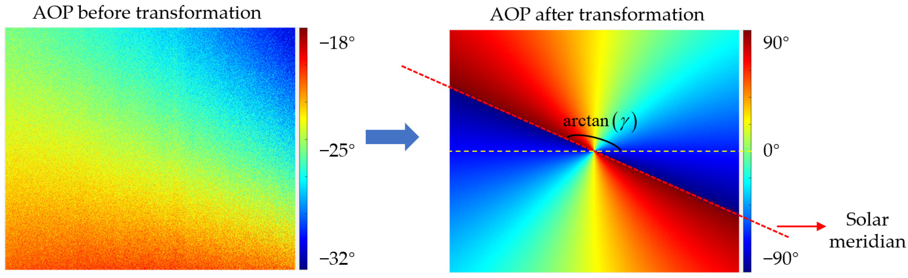
Notably, the value of the AOP is determined by the reference direction. The reference direction of the AOP calculated using Equation (20) is based on the direction of the 0° polarizer in the camera, making it difficult to visually observe the meridian from the AOP image. To calculate the solar azimuth angle, it is necessary to convert the reference direction of the AOP to the direction of the local meridian [31].

$$\mathrm{AOP}=\mathrm{AOP}\prime -\omega$$

(21)

where $\omega$ is the angle between the orientation of the 0° polarizer and the local meridian [32], which depends on the particle observed by the camera.

After transforming the coordinate system, the AOP image will display a distinct boundary line, as shown in Figure 8, which represents the solar meridian. This is due to the polarity change of the polarization angle near the solar meridian, transitioning from 90° to −90°, making the meridian a clear boundary line. By extracting points in the AOP that are close to ±90° and fitting them with least squares, the solar meridian can be determined. Then, by randomly selecting two points on this line, $\left(x_1,y_1\right)$ and $\left(x_2,y_2\right)$, the corresponding solar azimuth angle $A_s$ can be calculated as Equation (22).

$$A_s=\arctan \left(\gamma \right),\hspace{0.33em}\hspace{0.33em}\hspace{0.33em}\hspace{0.33em}\gamma ={\displaystyle \frac{y_2-y_1}{x_2-x_1}}$$

(22)

where $\gamma$ represents the slope of the meridian.

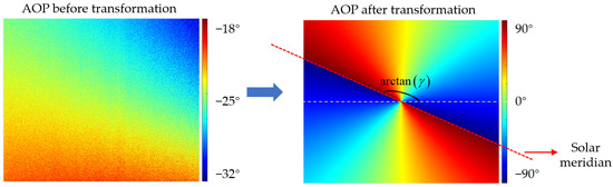
Figure 8. The schematic diagram of the AOP before and after coordinate transformation.

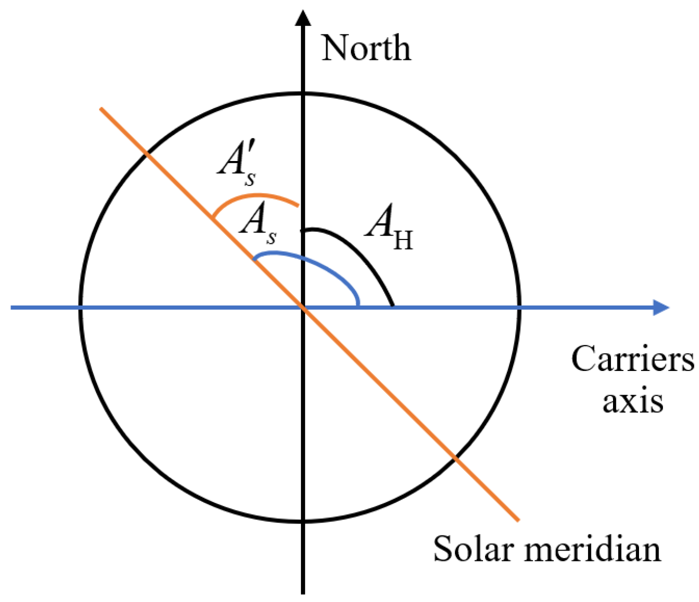
$A_s$ represents the sun’s position relative to the carrier in the carrier coordinate system. To achieve orientation, it is not sufficient to simply calculate $A_s$; we also need to find the angle between the carrier and a specific direction (true north). Then, based on the astronomical calendar, we determine the solar azimuth angle $A_s^{\prime }$ in the geographic coordinate system, which is expressed as Equation (23). $A_s^{\prime }$ indicates the sun’s position relative to true north. By combining $A_s$ and $A_s^{\prime }$ (Equation (24)), we can calculate the carrier’s position relative to true north $A_{\mathrm{H}}$, as shown in Figure 9, thus achieving the purpose of navigation.

$$A_s^{\prime }=\left\{\begin{array}{cc}\arccos \left({\displaystyle \frac{\sin h_s\sin L-\sin {\delta }_s}{\cos h_s\cos L}}\right)& T_s\le 0\\ {360}^{\circ }-\arccos \left({\displaystyle \frac{\sin h_s\sin L-\sin {\delta }_s}{\cos h_s\cos L}}\right)& T_s>0\end{array}\right.$$

(23)

$$A_{\mathrm{H}}=A_s-A_s^{\prime }$$

(24)

where $h_s$ is the solar altitude angle; $L$ is the geographical latitude of the observation point; ${\delta }_s$ and $T_s$ represent the solar declination angle and solar time angle, respectively; and $A_{\mathrm{H}}$ represents the heading angle.

Figure 9. The schematic diagram of the sun azimuth and heading angle.

4. Experiment and Results

To verify the feasibility of the proposed algorithm, relevant experiments were conducted. First, a bionic compass system was established to collect polarization information from the sky. Next, verification experiments were conducted on the polarization optimization model, demonstrating its ability to filter out disturbances from large particle scattering under non-ideal clear conditions. Finally, outdoor comparative experiments validated the effectiveness of the algorithm in determining heading.

4.1. Polarized Light Compass System

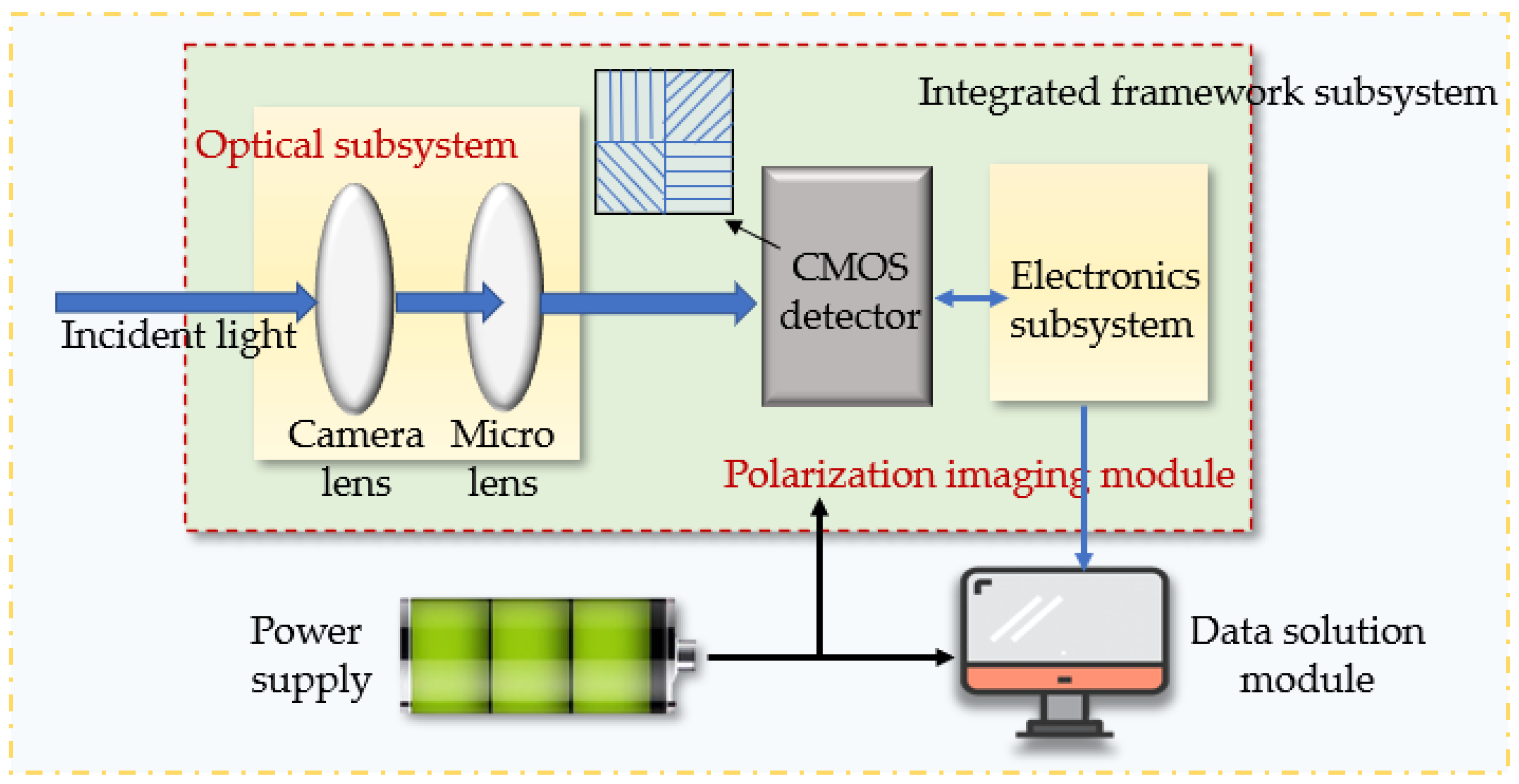
To determine the heading information of the body frame, a polarized light compass system was constructed. The system consisted of a polarization imaging module (polarized camera and optical lens), a power supply module, a data processing module, and an integrated framework subsystem. A schematic of the system structure is shown in Figure 10, and the parameters of the related components are listed in Table 1. For the outdoor polarization orientation experiment, the radiation energy from the sky was captured by the polarization imaging module and converted into digital images, which were output at a fixed frame rate. A computer was used as the data processing system, displaying the images from the polarization module in real-time and calculating the heading angle using the proposed algorithm. The integrated framework subsystem served as the outer shell of the entire compass system, consolidating various modules and concealing fragile components such as the camera and lens within the shell to protect them from external shocks and environmental influences. Additionally, the frame subsystem provided an information output interface for the real-time transmission of heading data. A portable power supply provided continuous power to both the imaging module and the data processing module. The camera was fixed on a high-precision turntable, which was used to rotate the camera and change its orientation, obtaining polarization data from multiple directions.

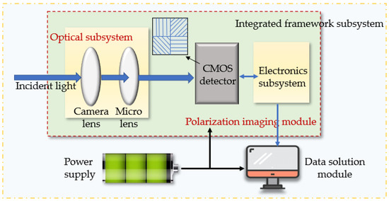
Figure 10. The schematic diagram of the bionic light compass system.

Table 1. Main devices involved in the outdoor experiment.

Experimental Instrument	Model and Manufacturer	Main Parameters
Division of focal-plane polarization camera	Lucid, PHX050S-P, Richmond, BC, Canada	Sony CMOS: IMX250MZR Resolution: 2048 × 2448
Industrial lens	Hikvision, MVL-HF2528M-6MP, Hangzhou, China	Focal length: 25 mm FOV: 32.6° × 21.8°
Power supply	Boltpower, Shenzhen, China	220 V, 300 W, 118,000 mAh
High-precision turntable	Honc, WFDT-360X, Shanghai, China	Accuracy: 0.005°

4.2. Polarization Optimization Model Validation Experiment

In this section, we present an outdoor calibration experiment to verify the advantages of the proposed polarization optimization model. The experiment was conducted at 5:00 p.m. on 27 March 2024 at the Beijing Institute of Technology (with its latitude and longitude obtained from Google Maps). On that day, the weather was cloudy with blowing sand, and the air quality index was 154 (moderate pollution). The atmosphere contained aerosols, water vapor, and dust particles, whose scattering effects weakened the sky polarization pattern information. Before the experiment, the camera underwent geometric and polarimetric calibration following the methods outlined in Refs. [33,34], respectively. The experimental setup is described in Section 4.1. The polarization images captured by the camera were processed using the optimization model described in Section 3.1 to calculate the optimized skylight polarization distribution pattern. A satellite positioning device (M100W, ComNav, Shanghai, China) was used to determine the camera’s true orientation, i.e., the heading angle. The solar altitude angle and solar azimuth angle in the carrier coordinate system were calculated by combining the heading angle and the astronomical calendar. Finally, the theoretical AOP image could be simulated based on the Rayleigh scattering model.

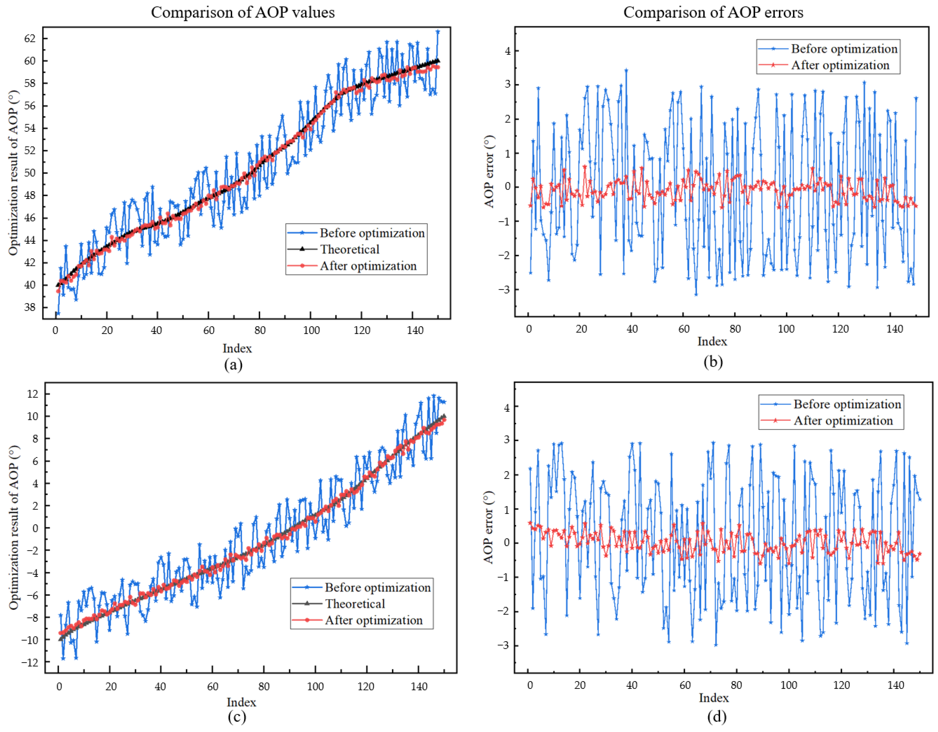
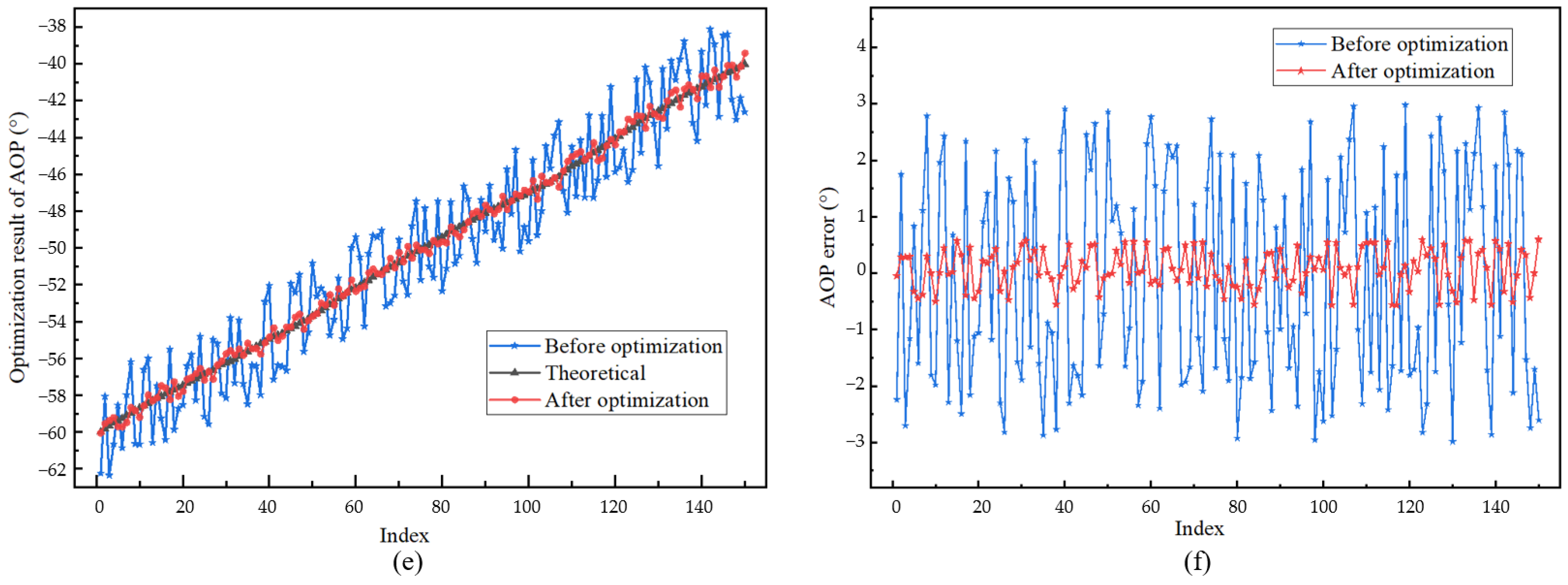
A pixel-wise comparison between the theoretical AOP and the measured AOP before and after optimization was conducted, with the results shown in Figure 11 and Table 2. The data in Figure 11a,c,e represent the AOP values of individual pixels. In these figures, the black line indicates the theoretical values obtained from simulations, the blue line represents the measured AOP values (without optimization), and the red line denotes the optimized measured values. Due to the large number of pixel values in the AOP images, only a randomly selected subset is presented. Figure 11a,c,e present theoretical AOP values in the ranges of 40–60, −10–10, and −60–−40, respectively. Figure 11b,d,f correspond to Figure 11a,c,e, showing the errors between the measured and theoretical AOP values. In Table 2, RMSE represents the root mean square error, calculated with Equation (25), which indicates the average deviation between the measured AOP and the theoretical AOP across all pixels. SSIM is the Structural Similarity Index, calculated with Equation (26), which represents the similarity between the measured AOP and the theoretical AOP.

$$\mathrm{RMSE}=\sqrt{{\displaystyle \frac{1}{N}}{\displaystyle \sum _{i=1}^N{\left(z-z^{\prime }\right)}^2}}$$

(25)

where $z$ is the predicted value, which here represents the AOP pixel value calculated based on the sky image; $z^{\prime }$ represents the truth value, which here denotes the AOP derived from Rayleigh scattering theory; and $N$ represents the number of samples.

$$\mathrm{SSIM}(Y,Y^{\prime })={\displaystyle \frac{(2{\mu }_Y{\mu }_{Y^{\prime }}+c_1)(2{\sigma }_{Y{Y}^{\prime }}+c_2)}{({\mu }_Y^2+{\mu }_{Y^{\prime }}^2+c_1)({\sigma }_Y^2+{\sigma }_{Y^{\prime }}^2+c_2)}}$$

(26)

where $Y$ represents the AOP image calculated based on the sky image and $Y^{\prime }$ represents the AOP image derived from Rayleigh scattering theory; ${\mu }_Y$ and ${\mu }_{Y^{\prime }}$ are the means of $Y$ and $Y^{\prime }$, respectively; ${\sigma }_Y^2$ and ${\sigma }_{Y^{\prime }}^2$ are variances of $Y$ and $Y^{\prime }$, respectively; ${\sigma }_{Y{Y}^{\prime }}$ represents the covariance of $Y$ and $Y^{\prime }$; and $c_1$ and $c_2$ are constants to maintain stability.

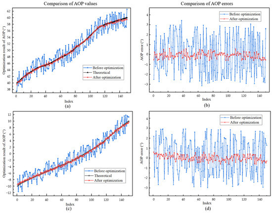
Figure 11. Comparison of the values and errors of the AOP before and after optimization and the theoretical AOP. (a,b) 40 to 60°; (c,d) −10 to 10°; and (e,f) −60 to −40°.

Table 2. Comparison of AOP errors before and after optimization.

	RMSE (°)	SSIM
Before optimization	6.3944	0.7638
After optimization	3.6120	0.9686

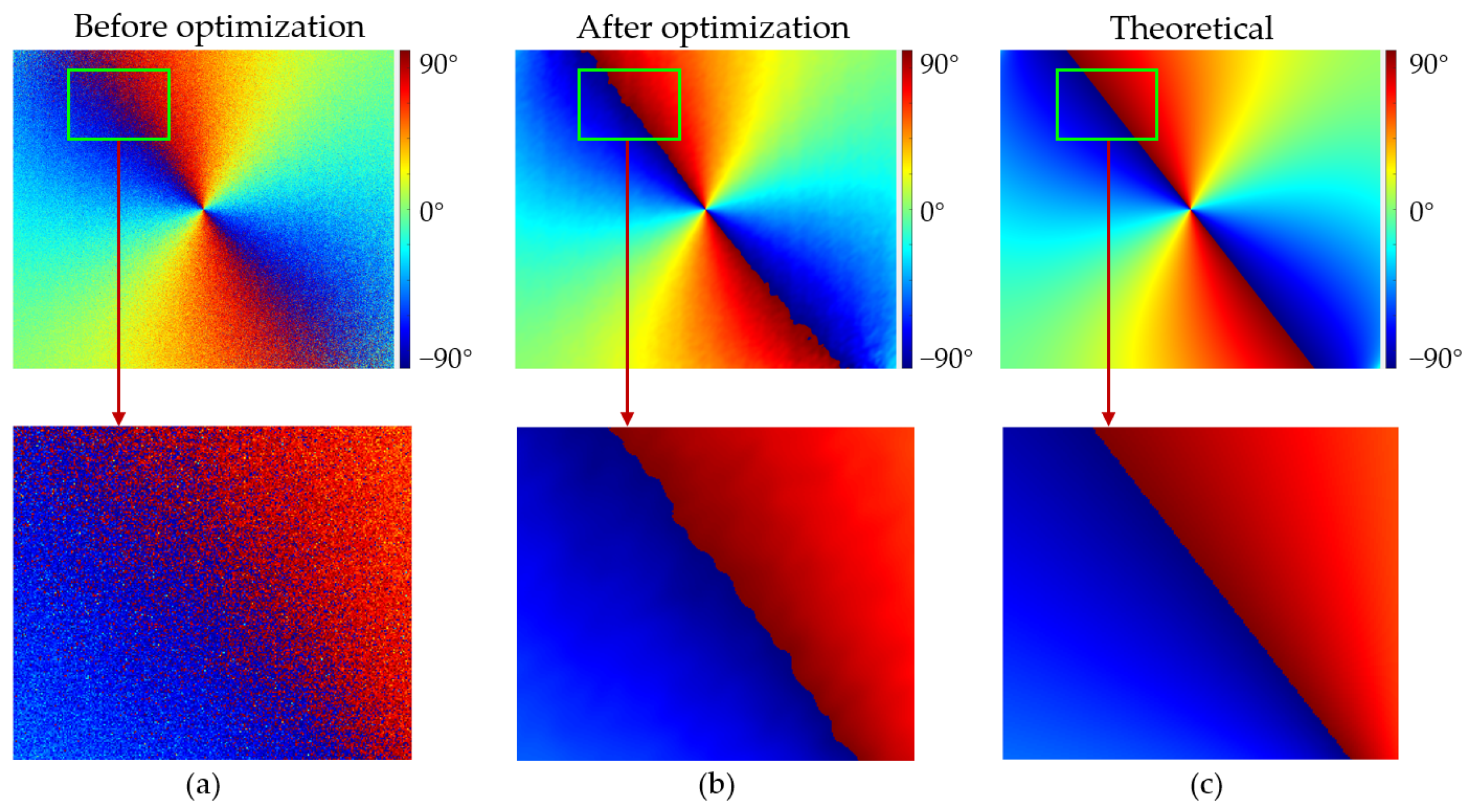
From Figure 11, it can be seen that the optimized AOP values were closer to the theoretical values, with significantly reduced errors and smoother error curves. The data in Table 2 further support this conclusion. Both the RMSE and SSIM indicate a substantial improvement in the AOP after optimization compared with the pre-optimization values. The RMSE of the optimized AOP error was 3.612°, representing a reduction of approximately 44%. The SSIM between the original AOP and the theoretical AOP was 0.7638, which increased to 0.9686 after optimization. Figure 12 shows a typical AOP image before and after optimization compared with the theoretical AOP image simulated according to Rayleigh scattering. According to the zoomed-in view of the AOP in Figure 12, the original AOP image (Figure 12a) exhibits considerable noise, especially around the meridian. Pixels of opposite polarity that should be separated by the meridian are intertwined with invalid pixels, resulting in a chaotic distribution that obscures the meridian, making it impossible to directly fit. After correction, the image is no longer blurry, the data distribution is more distinct, and the meridian is relatively clear, which is closer to the theoretical AOP image. By combining the data and images, we believe that the optimization model can mitigate the disturbances caused by large particles such as dust, thereby improving the accuracy of the AOP.

Figure 12. Comparison of AOP images before and after optimization and the theoretical AOP. (a) AOP image before optimization and its local magnification; (b) AOP image after optimization and its local magnification; and (c) theoretical AOP and its local magnification.

4.3. Outfield Validation Experiments of Heading Determination Algorithm

To verify the feasibility of the proposed method in heading determination, certain field comparison experiments were conducted. The experimental setup is described in Section 4.1, and the location is consistent with that in Section 4.2. The experimental scene is shown in Figure 13. Experiment 1 took place on 27 March 2024 at 5:00 p.m. under cloudy conditions with blowing sand, and the air quality index (AQI) was 154 (moderate pollution). Experiment 2 was conducted on 5 April 2024 at 4:00 p.m., with clear sky and some clouds, as well as an AQI of 69 (good). Experiment 3 took place at 11:30 a.m. on 3 April 2024 under overcast conditions, with an AQI of 73 (good).

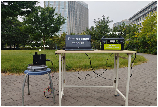
Figure 13. Experiment field with the designed polarization compass system.

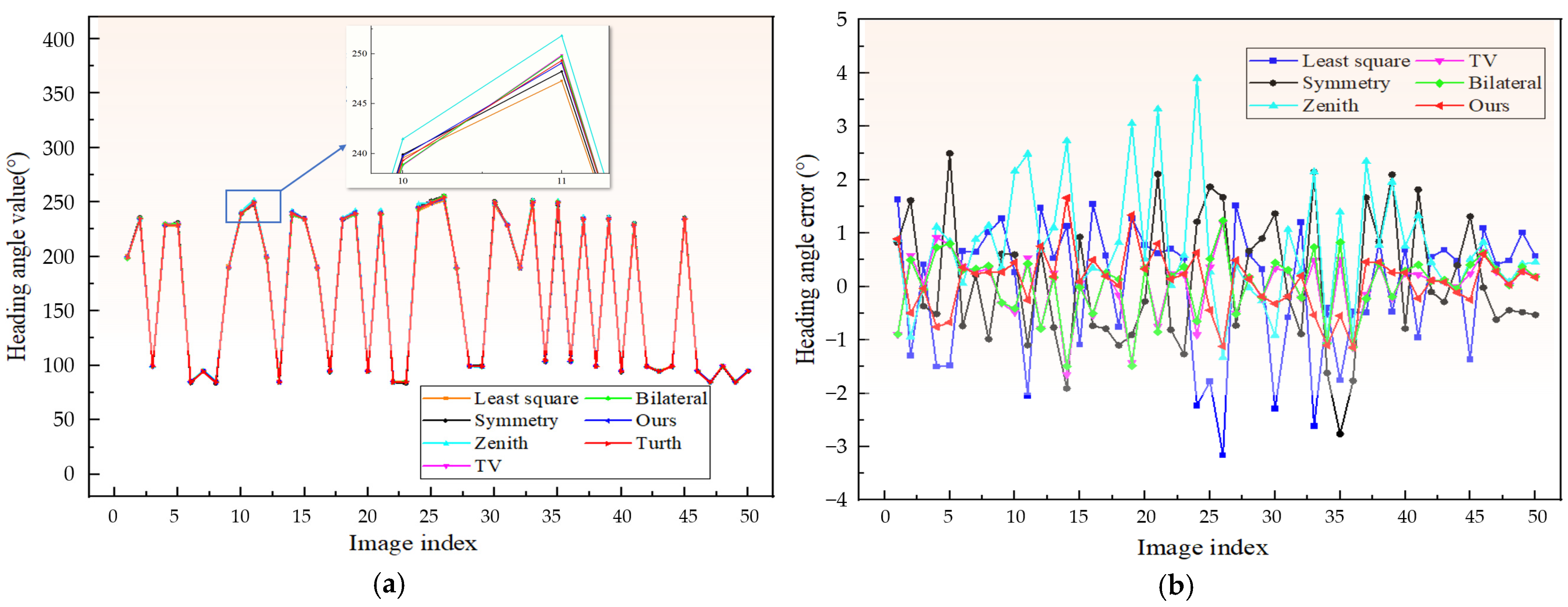
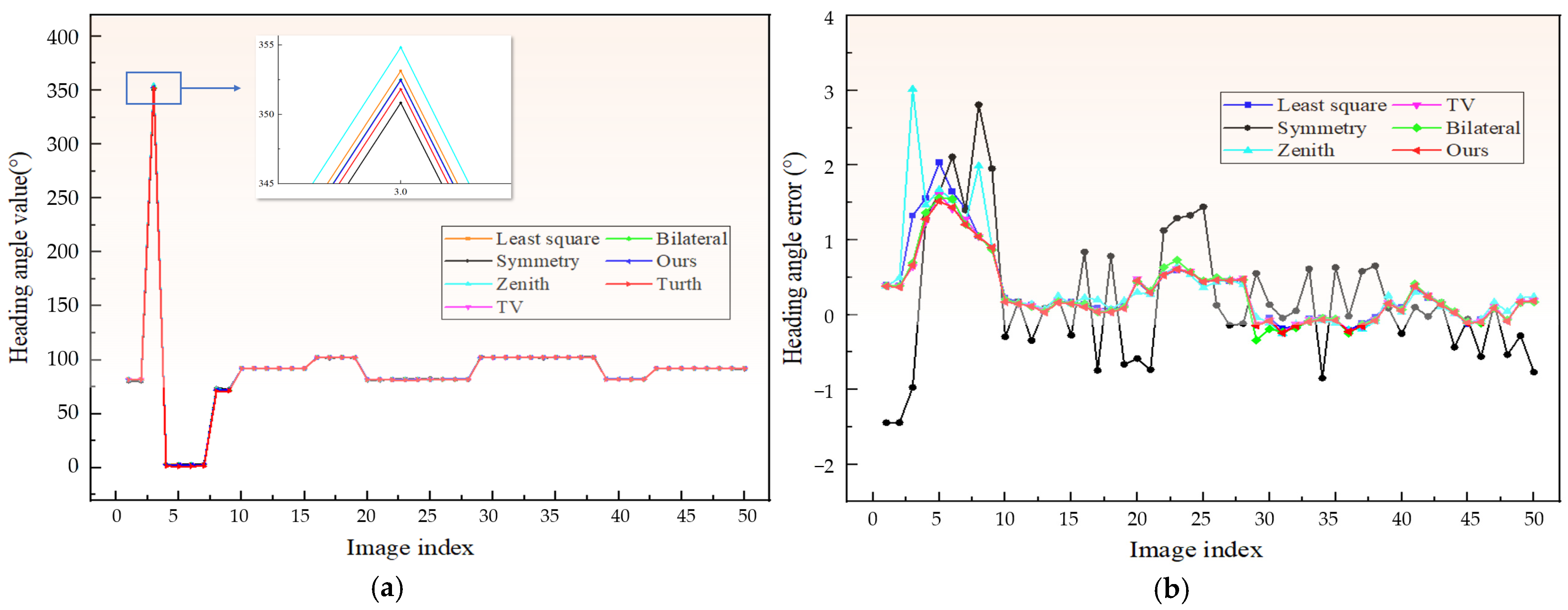
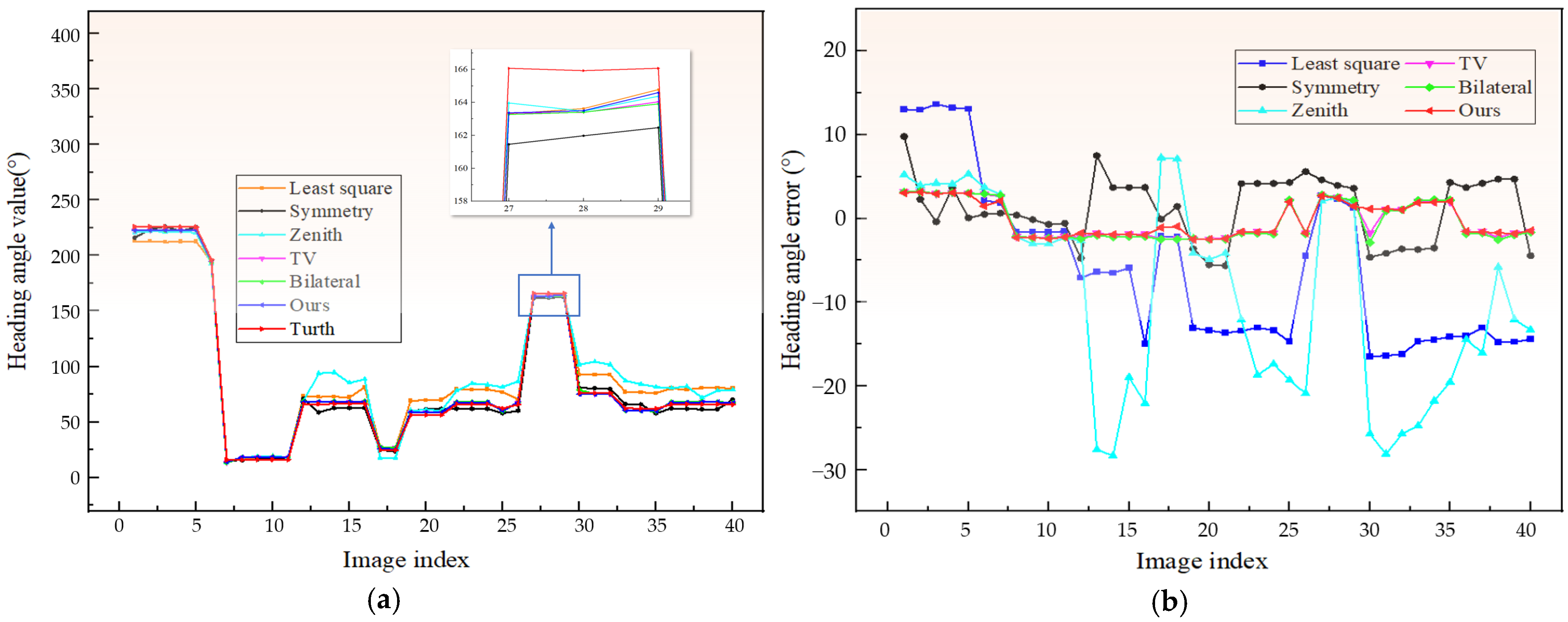
In the experiment, the camera was mounted on a high-precision turntable, and dynamic observation was achieved by rotating the turntable. The heading angle was calculated using the polarization orientation framework proposed in this paper, and the results were compared with the total variation (TV) denoising algorithm [26] and the bilateral filtering denoising algorithm [35,36], where the orientation component for both denoising algorithms was calculated using the method outlined in Section 3.2. Additionally, we compared our algorithm with three mainstream polarization orientation algorithms: the least squares method [6,7], the symmetry analysis method [13,14,15], and the zenith method [11,12]. The experimental results are shown in Figure 14, Figure 15 and Figure 16 and Table 3, Table 4 and Table 5.

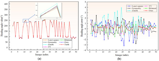
Figure 14. Heading measurement values and errors of Experiment 1. (a) Heading angle measurement values and their local magnification; (b) heading angle measurement errors.

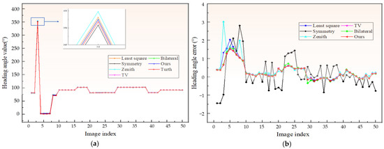
Figure 15. Heading measurement values and errors of Experiment 2. (a) Heading angle measurement values and their local magnification; (b) heading angle measurement errors.

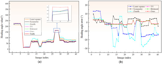
Figure 16. Heading measurement values and errors of Experiment 3. (a) Heading angle measurement values and their local magnification; (b) heading angle measurement errors.

Table 3. Heading measurement errors of Experiment 1.

	RMSE (°)	MAX (°)	Variance
Symmetry analysis	1.2173	−2.7652	1.5035
Zenith	1.3370	3.8972	1.2439
Least square	1.2248	−3.1656	1.5302
TV	0.584	−1.6485	0.34802
Bilateral	0.5912	−1.4955	0.3557
Ours	0.5594	1.661	0.3098

Table 4. Heading measurement errors of Experiment 2.

	RMSE (°)	MAX (°)	Variance
Symmetry analysis	0.9188	2.8096	0.8144
Zenith	0.7190	3.0191	0.3880
Least square	0.5998	2.0333	0.2577
TV	0.5156	1.605	0.1847
Bilateral	0.5313	1.5625	0.2028
Ours	0.5068	1.5188	0.1836

Table 5. Heading measurement errors of Experiment 3.

	RMSE (°)	MAX (°)	Variance
Symmetry analysis	4.0574	9.7940	15.4117
Zenith	14.8117	−28.3773	137.5910
Least square	11.2382	−16.5130	93.2443
TV	2.2245	3.2026	5.0226
Bilateral	2.3428	3.2160	5.5256
Ours	2.0664	3.1429	4.3537

In Experiment 2, the weather was clear, and the accuracy of all four methods was relatively high. Specifically, after the clouds completely cleared later in the experiment, the errors of the least squares, zenith, TV, bilateral and our proposed method were all within 0.2° while the symmetry analysis method had an error within 0.5°. This meets the basic requirements of heading calculation, especially for the self-alignment of vehicles [31].

In Experiment 1, the weather was cloudy with blowing sand and the atmosphere contained not only gaseous molecules but also larger particles like aerosols, water molecules, and dust. In Experiment 3, the weather was overcast, with a significant amount of cloud cover in the sky, and the air was filled with numerous cloud particles, including cloud droplets and ice crystals. Both conditions represent typical non-ideal weather. In both experiments, the accuracy of the least squares, zenith, and symmetry analysis methods all showed some decline. The scattering of dust introduced significant noise into the AOP image, generating a large number of invalid pixels and interfering with the identification of the meridian. The least squares method struggled to extract a complete set of feature points, making it difficult to fit an accurate meridian for heading determination. Cloud cover also disrupted the sky polarization pattern. When the center of the camera’s field of view was obscured by cloud cover, the zenith region of the sky was affected by both clouds and dust, resulting in erroneous data. This reduced the accuracy of the zenith method and could even render it ineffective; in Experiment 3, the maximum error of the zenith method reached as high as −28.3773°. For the symmetry analysis method, the invalid pixels introduced by dust disrupted the symmetry of the AOP. The presence of clouds exacerbated this disruption, especially when the clouds were concentrated on one side of the solar or anti-solar meridian, leading to even greater disruption.

The least squares, zenith, and symmetry analysis methods have limitations that cannot be overcome; in contrast, the method presented in this paper demonstrates notable advantages, especially as demonstrated in Experiment 3. As shown in Figure 14, Figure 15 and Figure 16 and Table 3, Table 4 and Table 5, regardless of sunny, cloudy, or blowing conditions, our method maintained a high accuracy, with an average error kept within 1° and around 2° even in overcast conditions. In this study, the algorithm employed a polarization optimization model to eliminate disturbances from larger particles such as aerosols and dust. It restored the original sky polarization pattern as much as possible, enhancing both symmetry and the clarity of the meridian. Several representative images are shown in Figure 17. Compared with the other two denoising algorithms, our method was more accurate in heading determination. In Experiment 1, our algorithm showed accuracy improvements of 4.2% and 5.4% over the TV denoising and bilateral filtering algorithms, respectively. In Experiment 2, our accuracy increased by 1.7% and 4.6%, and in Experiment 3, it increased by 7.1% and 11.8%. Additionally, when compared with the three mainstream polarization orientation methods, our algorithm demonstrated accuracy improvements of 54.1%, 58.1%, and 54.3% in Experiment 1; 44.8%, 29.5%, and 15.5% in Experiment 2; and 49.1%, 86.1%, and 81.6% in Experiment 3. These results confirm the robustness and promising application potential of the proposed method.

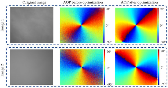
Figure 17. Schematic diagram of the sample image and its sky polarization distribution pattern in the orientation experiment.

5. Conclusions

Even in sunny weather conditions, the accuracy of polarization navigation can still be affected by the presence of large particles such as aerosols and clouds. Therefore, this paper proposes a bionic navigation method based on atmospheric polarization optimization to improve heading accuracy under non-ideal clear conditions. The disturbances from particles like aerosols are incorporated into the raw signal captured by the camera, establishing a signal model for non-ideal clear conditions. On this basis, an energy functional optimization model is constructed to restore the original sky polarization pattern. In addition, a bionic optical compass system was constructed. Navigation experiments under sunny, cloudy and sandy conditions demonstrated the superiority of the proposed method.

There are, however, some limitations in our work. This study is only applicable to weather conditions with relatively low concentrations of particulate matter, such as clear skies, cloudy days, and blowing sand. In extreme weather events like sandstorms, the concentration of particulate matter rises sharply, causing the AQI to spike to “severe pollution” (above 300). Under such conditions, the sky polarization model is completely and severely disrupted, making it difficult for the optimized model to achieve accurate restoration. In the future, we aim to further refine the algorithm to handle extreme conditions like sandstorms, expanding its range of applications.

References

- Suhai, B.C.; Horváth, G. How well does the Rayleigh model describe the E-vector distribution of skylight in clear and cloudy conditions? A full-sky polarimetric study. J. Opt. Soc. Am. A 2004, 21, 1669–1676. [Google Scholar] [CrossRef] [PubMed]
- Zhou, Y.C.; Ye, C.; Lin, Z.H.; Zhan, C.L.; Gao, H. Self-Adaptive Image Segmentation Algorithm for Polarization Navigation under Complex Scenes. Acta Opt. Sin. 2024, 44, 150–160. [Google Scholar]
- Wang, D.; Liang, H.; Zhu, H.; Zhang, S. A bionic camera-based polarization navigation sensor. Sensors 2014, 14, 13006–13023. [Google Scholar] [CrossRef] [PubMed]
- Lambrinos, D.; Möller, R.; Labhart, T.; Pfeifer, R.; Wehner, R. A mobile robot employing insect strategies for navigation. Robot. Auton. Syst. 2000, 30, 39–64. [Google Scholar] [CrossRef]
- Liang, H.; Bai, H.; Hu, K.; Lv, X. Bioinspired polarized skylight orientation determination artificial neural network. J. Bionic Eng. 2023, 20, 1141–1152. [Google Scholar] [CrossRef]
- Wang, Y.; Yang, J.; Tang, J.; Liu, J.; Sheng, C.; Qin, L. Heading angle detection system based on atmospheric polarized light. J. Ordnance Equip. Eng. 2019, 40, 127–131. [Google Scholar]
- Wang, C.; Zhang, N.; Li, D.; Yang, J.; Wang, F.; Ren, J.; Tang, J.; Liu, J.; Xue, C. Calculation of heading angle using all-sky atmosphere polarization. Opto-Electron. Eng. 2015, 42, 60–66. [Google Scholar]
- Aycock, T.; Lompado, A.; Wolz, T.; Chenault, D. Passive optical sensing of atmospheric polarization for GPS denied operations. Proc. SPIE 2016, 9838, 98380Y. [Google Scholar]
- Wang, X.; Gao, J.; Fan, Z. Empirical corroboration of an earlier theoretical resolution to the UV paradox of insect polarized skylight orientation. Naturwissenschaften 2014, 101, 95–103. [Google Scholar] [CrossRef]
- Aycock, T.M.; Lompado, A.; Wheeler, B.M. Using atmospheric polarization patterns for azimuth sensing. Proc. SPIE 2014, 9085, 90850B. [Google Scholar]
- Dupeyroux, J.; Viollet, S.; Serres, J.R. Polarized skylight based heading measurements: A bio-inspired approach. J. R. Soc. Interface 2019, 16, 20180878. [Google Scholar] [CrossRef] [PubMed]
- Dupeyroux, J.; Viollet, S.; Serres, J.R. An ant-inspired celestial compass applied to autonomous outdoor robot navigation. Robot. Auton. Syst. 2019, 117, 40–56. [Google Scholar] [CrossRef]
- Ma, T.; Hu, X.; Zhang, L.; Lian, J.; He, X.; Wang, Y.; Xian, Z. An evaluation of skylight polarization patterns for navigation. Sensors 2015, 15, 25746–25760. [Google Scholar] [CrossRef]
- Liang, H.; Bai, H.; Sun, R.; Sun, R.; Guo, H. Polarization orientation determination algorithm based on the extremum of moment of inertia. In Proceedings of the Chinese Control Conference, Wuhan, China, 25–27 July 2018; pp. 4928–4932. [Google Scholar]
- Zhao, H.; Xu, W.; Zhang, Y.; Li, X.; Zhang, H.; Xuan, J.; Jia, B. Polarization patterns under different sky conditions and a navigation method based on the symmetry of the AOP map of skylight. Opt. Express 2018, 22, 28589–28603. [Google Scholar] [CrossRef]
- Jiang, R.; Wang, X.; Zuo, Y. Research on bionic navigation based on local atmospheric polarization. Acta Aeronaut. Astronaut. Sin. 2020, 41, 152–160. [Google Scholar]
- Li, Y.; Wang, X.; Pan, Y.; Li, L.; Chen, J. Ultraviolet-visible light compass method based on local atmospheric polarization characteristics in adverse weather conditions. Appl. Opt. 2022, 61, 6853–6860. [Google Scholar] [CrossRef]
- Li, Y.; Wang, X.; Zhang, M.; Xu, C. Ultraviolet bionic compass method based on non-ideality correction and statistical guidance in twilight conditions. Opt. Express 2024, 32, 22132–22152. [Google Scholar] [CrossRef]
- Tang, J.; Zhang, N.; Li, D.; Wang, F.; Zhang, B.; Wang, C.; Shen, C.; Ren, J.; Xue, C.; Liu, J. Novel robust skylight compass method based on full-sky polarization imaging under harsh conditions. Opt. Express 2016, 24, 15834–15844. [Google Scholar] [CrossRef]
- Wu, X.D.; Zhao, D.H.; Yu, H.; Jin, T.; Liu, Y.X.; Shen, C. Bionic Polarization Orientation Method Under Severe Weather. J. Navig. Position. Timing. 2022, 9, 104–111. [Google Scholar]
- Li, Q.; Hu, Y.; Hao, Q.; Cao, J.; Cheng, Y.; Dong, L.; Huang, X. Skylight polarization patterns under urban obscurations and a navigation method adapted to urban environments. Opt. Express 2021, 29, 42090–42105. [Google Scholar] [CrossRef]
- Zhang, R.; Cai, H.; Guan, L.; Wan, Z.-H.; Chen, Y.-T.; Fan, Y.-Y.; Chu, J.-K. Polarization orientation method for cloudy sky. Opt. Precis. Eng. 2021, 29, 1499–1510. [Google Scholar] [CrossRef]
- Pu, X.; Wang, X.; Gao, X.; Wei, C.; Gao, J. Sky Polarization Pattern Reconstruction and Neutral Line Detection Based on Adversarial Learning. IEEE Trans. Instrum. Meas. 2023, 72, 1–13. [Google Scholar] [CrossRef]
- Li, X.; Zhang, R.; Lu, S.F.; Lin, M.; Chu, J. Ultraviolet Polarization Employing Mie Scattering Monte-Carlo Method for Cloud-Based Navigation. Laser Optoelectron. Prog. 2021, 58, 1701001. [Google Scholar]
- Wu, X.D. Study on Orientation of Atmospheric Polarized Light in Complex Weather; North University of China: Taiyuan, China, 2022. [Google Scholar]
- Rudin, L.; Osher, S.; Fatemi, E. Nonlinear total variation based noise removal algorithms. Physica D 1992, 60, 259–268. [Google Scholar] [CrossRef]
- Wang, J.; Chen, R.; Ma, X.Q.; Wu, B.Y. Unsupervised seismic data random noise suppression method based on weighted total variation regularization and ADMM solution. Oil Geophys. Prospect. 2023, 58, 769–779. [Google Scholar]
- Grippo, L.; Sciandrone, M. Globally convergent block-coordinate techniques for unconstrained optimization. Optim. Methods Softw. 1999, 10, 587–637. [Google Scholar] [CrossRef]
- Beck, A.; Tetruashvili, L.; Vaisbourd, Y.; Shemtov, A. Rate of convergence analysis of dual-based variables decomposition methods for strongly convex problems. Oper. Res. Lett. 2016, 44, 61–66. [Google Scholar] [CrossRef]
- Zhang, N.; Chu, J.; Zhao, K.; Meng, F. The design of the subwavelength wire-grid polarizers based on rigorous couple-wave theory. Chin. J. Sens. Actuators 2006, 19, 1739–1743. [Google Scholar]
- Liang, H.; Bai, H.; Liu, N.; Sui, X. Polarized skylight compass based on a soft-margin support vector machine working in cloudy conditions. Appl. Opt. 2020, 59, 1271–1279. [Google Scholar] [CrossRef]
- Lu, H.; Zhao, K.; Wang, X.; You, Z.; Huang, K. Real-time imaging algorithm orientation determination system to verify imaging polarization navigation. Sensors 2016, 16, 562. [Google Scholar] [CrossRef]
- Zhang, Z.Y. A flexible new technique for camera calibration. IEEE Trans. Pattern Anal. Mach. Intell. 2000, 22, 1330–1334. [Google Scholar] [CrossRef]
- Xu, Z.Y. Polarization Image Preprocessing and Objective Evaluation Method of Fused Image; Beijing Institute of Technology: Beijing, China, 2019. [Google Scholar]
- Tomasi, C.; Manduchi, R. Bilateral filtering for gray and color images. In Proceedings of the 6th International Conference on Computer Vision, Bombay, India, 7 January 1998; pp. 839–846. [Google Scholar]
- Hao, J.; Du, Y.; Wang, S.; Ren, W. Infrared image enhancement algorithm based on wavelet transform and improved bilateral filtering. Infrared Technol. 2024, 46, 1051–1059. [Google Scholar]
Disclaimer/Publisher’s Note: The statements, opinions and data contained in all publications are solely those of the individual author(s) and contributor(s) and not of MDPI and/or the editor(s). MDPI and/or the editor(s) disclaim responsibility for any injury to people or property resulting from any ideas, methods, instructions or products referred to in the content. |
© 2024 by the authors. Licensee MDPI, Basel, Switzerland. This article is an open access article distributed under the terms and conditions of the Creative Commons Attribution (CC BY) license (https://creativecommons.org/licenses/by/4.0/).