Enhanced Clustering MAC Protocol Based on Learning Automata for UV Networks

Abstract

Ultraviolet (UV) networks are widely applied in complex electromagnetic environments. Designing an efficient multi-node medium access control (MAC) protocol for these networks is important. In this study, we proposed an enhanced clustering time division multiple access (TDMA) MAC protocol based on clustering and learning automata (LA). Subsequently, the effects of the network topology, class of service, and number of cluster nodes on the network performance under the proposed protocol were analyzed. Then, the protocol was compared with the TDMA protocol and clustering system. Results revealed that it obtained a better network performance, proving its suitability for multi-node UV networking.

1. Introduction

Ultraviolet (UV) networks are mobile networks that use UV radiation as communication carriers to realize wireless multi-hop communication among UV communication terminals [1]. These networks can be applied to military networks, emergency services, disaster recovery, and other complex electromagnetic environments due to their excellent non-line-of-sight (NLOS) communication, high security, and all-weather operation [2]. The secure properties of UV networks include strong anti-interference abilities, good confidentiality, and low position resolutions [3]; thus, they have recently become a research hotspot [4]. Unfortunately, high-power UV light sources cause damage to the eyes and skin; therefore, the power of the light source should be strictly controlled according to safety regulations [5].

Properly setting up and optimizing the media access control (MAC) protocol is significant in improving network performance [6]. This protocol is one of the key technologies for realizing communication through UV networks. At present, the UV MAC protocols are relatively lacking and fall into two main categories [5,7]. The first class concerns competition-based protocols, which require less control overhead and are more suitable for changes in network topology [8]. However, as traffic loads increase, there are more transmission collisions, resulting in the network performance significantly deteriorating. Furthermore, competition-based protocols do not ensure the quality of service (QoS) and bounded network delays in highly dense scenarios.

On the other hand, the second class has received increasing attention. In competition-free MAC protocols, a certain channel is allocated to a single terminal at a time. When a terminal transmits data in this channel, no other terminal competes for channel resources. The competition-free protocol can guarantee the QoS of the data, and its performance is better than that of the competition-based MAC protocol under a high traffic load. Liu et al. [9] proposed that the competition-free protocol had a better QoS than the competition-based protocol that worked based on the carrier sense multiple access (CSMA) mechanism.

Studies on using a competition-free MAC protocol have been carried out to provide an optimized access mechanism in the bandwidth-constrained solar-blind UV band [10]. Compared to other MAC protocols, the time division multiple access (TDMA) protocol is a representative competition-free protocol with several preponderances, such as convenient networking, good communication reliability, and bounded network delay [11]. However, there is an unavoidable defect in this protocol regarding its fixed-slot allocation, that is, the time slot allocated to the terminals is inversely proportional to the number of nodes, resulting in a longer network delay and unsatisfactory throughput in multi-node networks [12].

The traditional TDMA protocol can be improved by employing the concept of clustering in cognitive radio ad hoc networks [13]. In the clustering protocol, the number of nodes that interfere with one another is limited, solving the problem of the network performance rapidly deteriorating as the number of nodes increases [14]. Moreover, this protocol provides convenient topology adjustments in the cluster [15,16].

In practical network scenarios, the load and channel resource requirements of each terminal significantly vary, and the fixed-slot allocation mechanism cannot fully utilize the channel. Therefore, in this study, we optimized the clustering mechanism even further using a reinforcement learning (RL) algorithm. To address the channel utilization problem, the cluster leader (CL) uses a smart learning automata (LA) model to monitor the intracluster transmissions and learn the traffic parameters of its cluster nodes (CNs), avoiding any complications [17]. The LA can help the CL optimize the allocation of intracluster time slots, thereby maximizing the channel utilization.

The main contents of the paper include:

(1)

An enhanced clustering TDMA MAC protocol based on LA (CL-LA MAC) was proposed for UV networks, wherein the network topology of the clustering mechanism and dynamic slot allocation of the RL algorithm were combined.

(2)

The variation of the cache queue length was mathematically analyzed using a Markov chain (MC), and the stable cache probability distributions for CL and CN were derived separately to analyze the network performance.

(3)

The effects of the network topology, class of service, and number of CNs on the network performance under the CL-LA MAC protocol were analyzed. Compared with the conventional TDMA protocol and clustering system, a better network performance was achieved under the CL-LA system wherein the clustering topology and dynamic time slot allocation mechanism were employed, proving the effectiveness of the proposed protocol.

2. Learning Automata

Under the CL-LA protocol, the LA located at the CLs constantly update their output behavior through repeated interaction learning with the random environment until they obtain the behavior that is most suitable for the random environment to help the CLs optimally allocate the intracluster time slot to the CNs and maximize the channel utilization.

The LA are decision-making units under the RL [18]. An adaptive decision-making mechanism comprises an LA and external environment, and the decision system can adjust its responses based on past experiences. This system can choose the best action based on the reward or penalty characteristics of the random environment to improve the overall performance. Specifically, an action is randomly selected as an input to the environment based on the updated probability distribution for each step. The LA adjusts their state and updates their probability distributions according to the reinforcement feedback provided by the environment and they then converge to the optimal behavior [19,20].

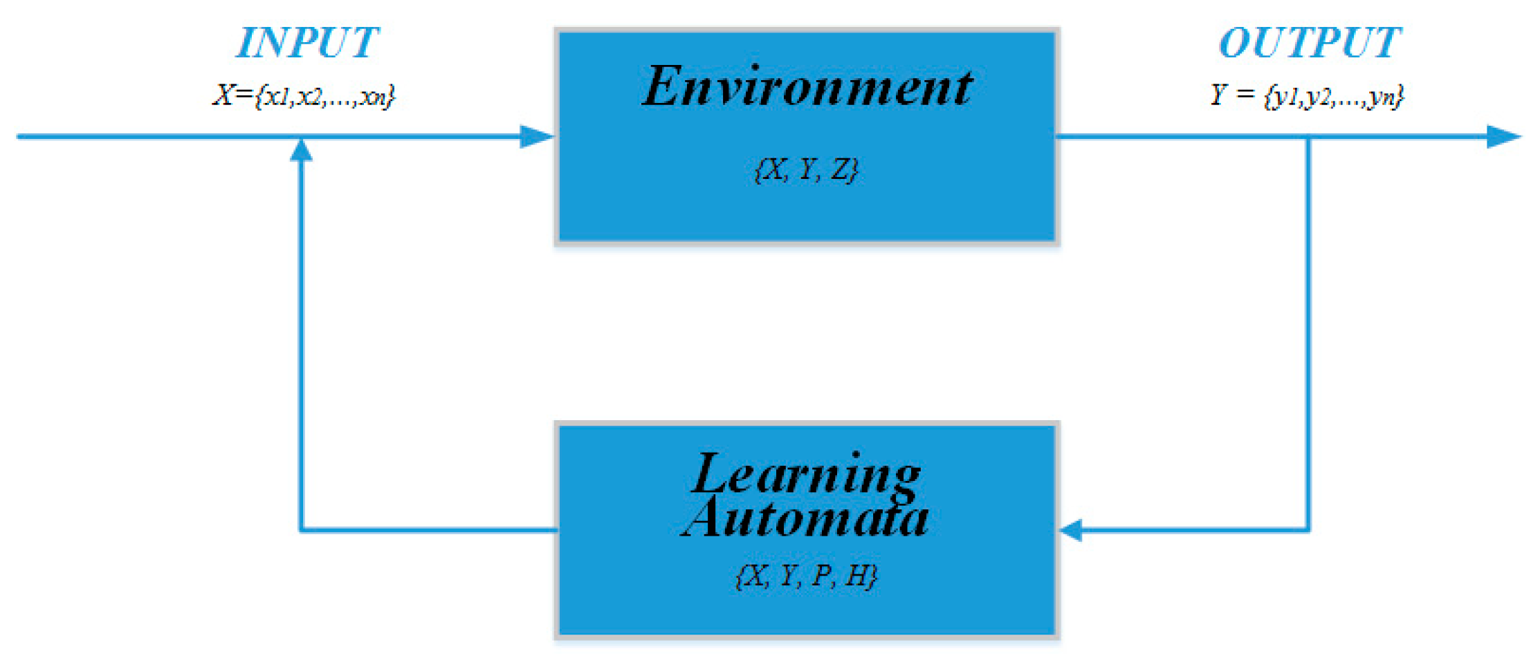
The system model consists of an LA and a random environment, which form a closed loop through the action and feedback. The interaction diagram of the LA and random environment is shown in Figure 1.

The core idea of linear LA algorithms is that the probabilities of selected actions are updated when the decision system receives rewards or penalties from the environment [21]. The environment can be defined by a triple {X, Y, Z}, where X = {x₁, x₂, …, x_n} specifies a set of n inputs that forms the action set of the LA, and n is the maximum number of possible actions. One action, x_i, from set X is selected and inputted into the random environment at each iteration. The set Y = {y₁, y₂, …, y_n} is the output after reinforcement feedback, which is the feedback set of the random environment, and the set Z = {z₁, z₂, …, z_n} represents n reward probabilities corresponding to each action in set X.

The variable types of LA can be defined as a quadruple {X, Y, P, H}, where X = {x₁, x₂, ..., x_n} is a set of n actions, Y = {y₁, y₂, ..., y_n} indicates a set of LA inputs, P = {p₁, p₂, …, p_n} refers to the action probability vector, and H: p_i(t + 1) = H[x_i(t), y_i(t), p_i(t)] is a learning algorithm.

Under the LA algorithm used in this study, the linear reward–penalty (L_RP) scheme was used to update the action probability on the feedback in the form of rewards and penalties. This is shown in Algorithm 1. When the selected action x_i was rewarded, the corresponding action probability increased, whereas the probabilities of the other actions decreased, as shown in (1).

$$p_s(t+1)=\left\{\begin{array}{c}{p}_s(t)+\alpha \cdot [1-p_s(t)],s=i\\ (1-\alpha )\cdot p_s(t),\forall s\ne i\end{array}\right..$$

(1)

Conversely, the corresponding action probability decreased when the selected action x_i was penalized, whereas the probabilities of the other actions increased according to (2).

$$p_s(t+1)=\left\{\begin{array}{r}\hfill (1-\beta )\cdot p_s(t),s=i\\ \hfill \frac{\beta }{n-1}+(1-\beta )\cdot p_s(t),\forall s\ne i\end{array}\right.,$$

(2)

where α and β are the reward and penalty parameters, respectively, and t is the number of cycles.

Algorithm 1. Algorithm of LRP.

Input: Reward parameter α and penalty parameter β

1: Initialization      Action probability vector pi = 1/n, $\forall i\in [0,n]$

2: Repeat 3:    At cycle t, the action xi is chosen according to the action probability vector P 4:    Obtain feedback Yi(t) from the environment on the selected action xi 5: if         Yi(t) = 1      then 6:    Update the action probability vector P according to the reward formula

7:        $p_s(t+1)=\left\{\begin{array}{c}{p}_s(t)+\alpha \cdot [1-p_s(t)],s=i\\ (1-\alpha )\cdot p_s(t),\forall s\ne i\end{array}\right..$   # xi is rewarded 8: else if    Yi(t) = 0 9:    Update the action probability vector P according to the penalty formula

10:      $p_s(t+1)=\left\{\begin{array}{r}\hfill (1-\beta )\cdot p_s(t),s=i\\ \hfill \frac{\beta }{n-1}+(1-\beta )\cdot p_s(t),\forall s\ne i\end{array}\right..$   # xi is penalized

11: end if

12: Until   max{pi(t)} > 0.99

3. CL-LA MAC Protocol

The nodes were divided into independent clusters. Each cluster had a CL that processed and forwarded the data of the CNs. This clustering mechanism could avoid conflicts caused by providing concurrent access to the same available time slot, limiting the number of terminals that interfered with one another, and providing fair channel access and effective topological control in a cluster. Additionally, with the support of the LA algorithm, the CL could flexibly and dynamically allocate the intracluster time slots for CNs, avoiding wasteful gaps between the time slots and improving the channel utilization.

A.

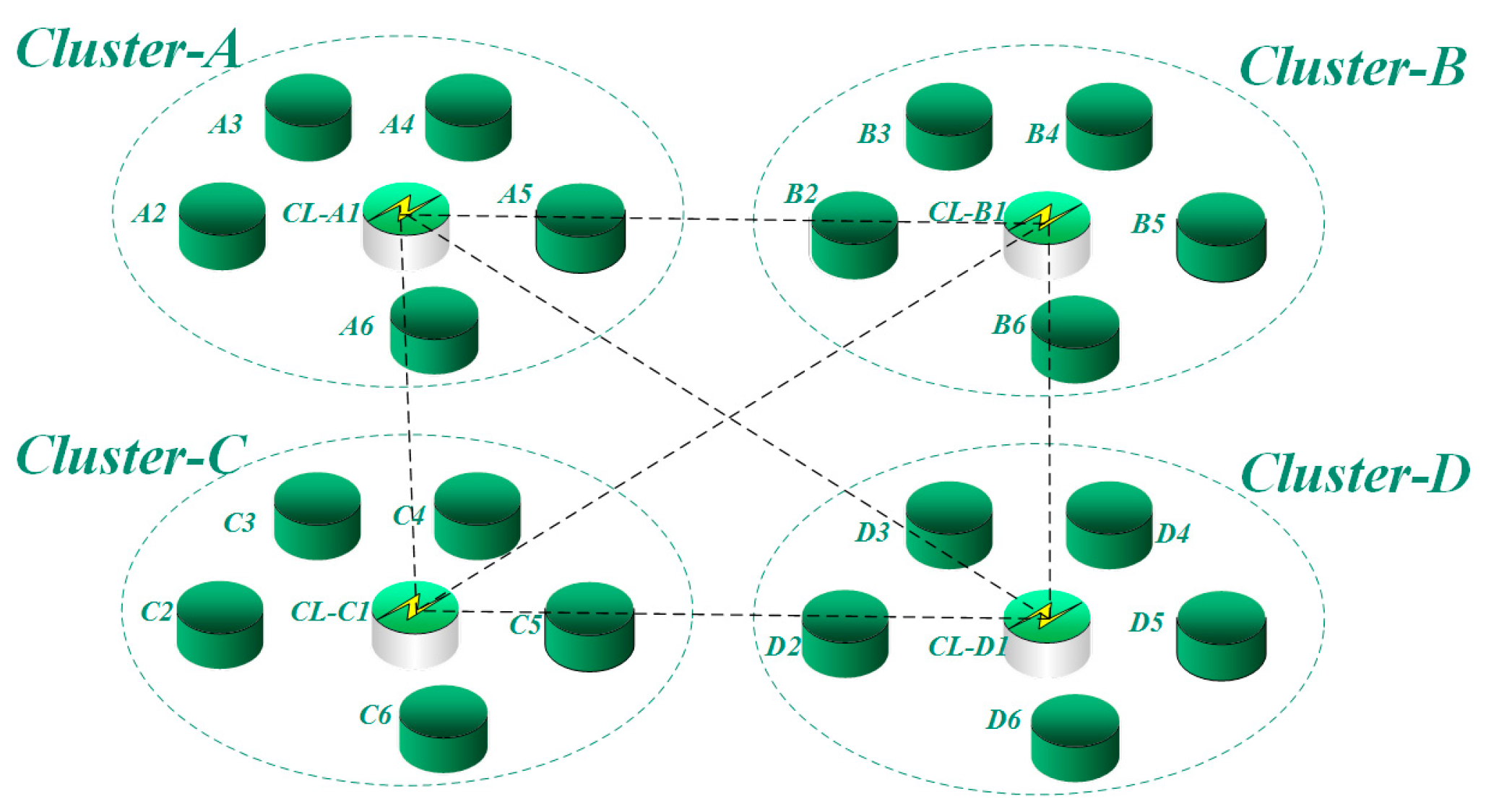
Network model

Figure 2 shows a twenty-four node network model. The network is divided into four clusters wherein nodes A1, B1, C1, and D1 are CLs, and the others are CNs. The CLs could communicate with one another. The CNs could only communicate with other CNs within the same cluster. CNs belonging to different clusters established communication by forwarding information through the CLs. Taking the communication between CN-A2 and CN-B2 as an example; first, A2 would send data to CL-A1 in the allocated time slot. Then, the data would be stored in A1 and transmitted to B1 in the transmission time slot of A1. Finally, the data would be forwarded from B1 to B2. The information flow for this case would be A2-A1-B1-B2.

B.

Working modes

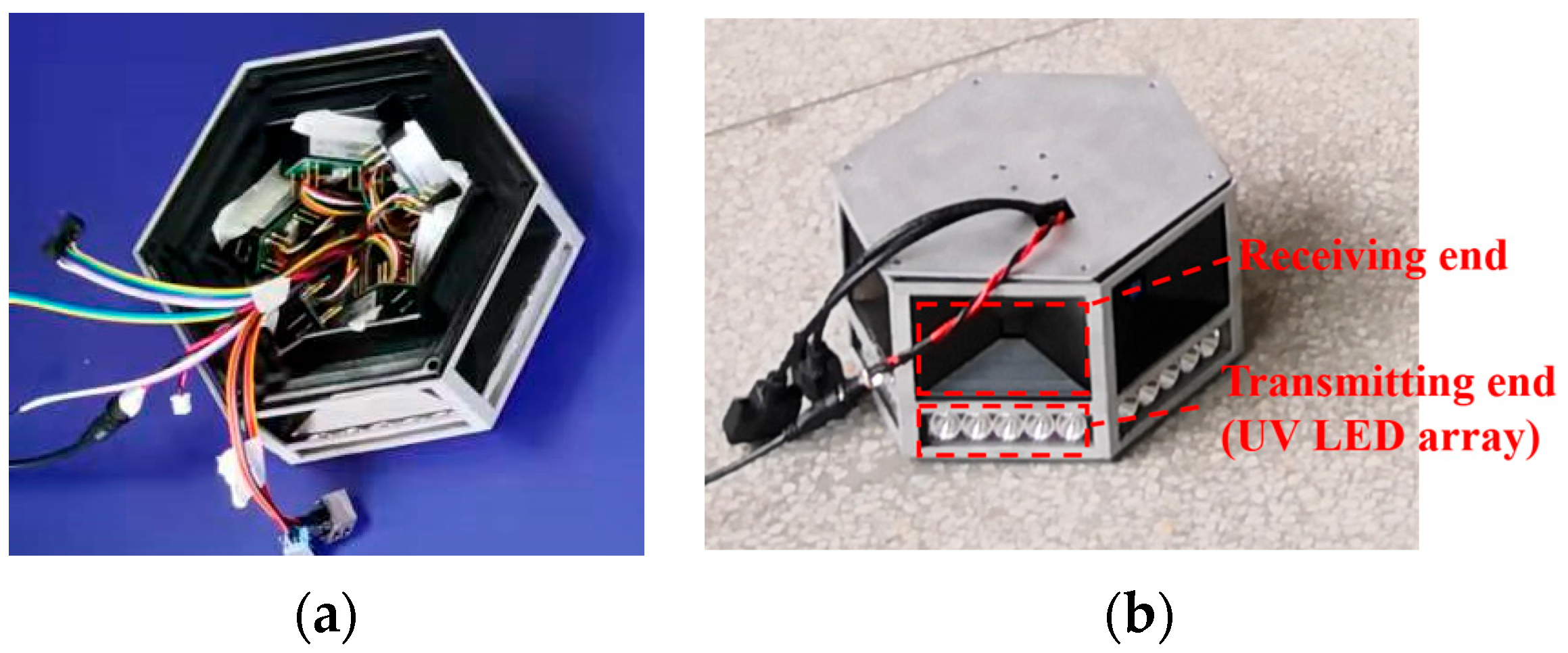
In the clustering network, different working modes can be adopted for the CLs and CNs. The CN model is a hexagonal body, and each side has separate transmitting and receiving devices, as shown in Figure 3. Within each cluster, the approximate positions of adjacent nodes can be predicted, and a neighbor table can be formed for a specific CN. Using this table, the CN can select a UV light-emitting diode (LED) array on the corresponding side to directionally send data to the target node with a low transmission power, saving energy and prolonging the service life of the UV nodes.

Omnidirectional transmission was selected for the CL to facilitate its communication with other CLs and forward the information from CNs. Since the entire network was based on the clustering-based TDMA mechanism, and there was no interference among the nodes, and all the nodes adopted an omnidirectional receiving mode.

C.

Allocation of intracluster time slots

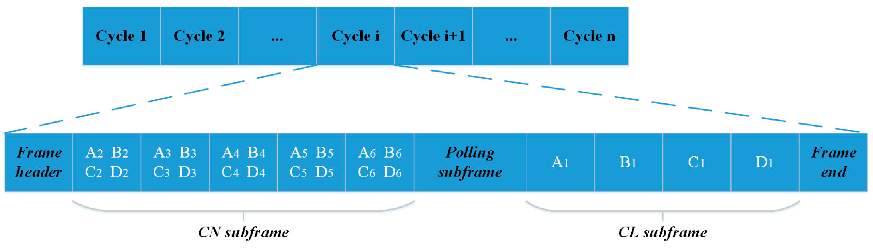
The data frame consists of a frame header, CN subframe, polling subframe, CL subframe, and frame end, as shown in Figure 4. The CN subframe was dynamically allocated to CNs by the corresponding CL. The CL polled the CNs in the polling subframe. According to the polling results and updated output of the LA, the CL broadcasted new mapping information among the CNs and their allocated slots in the next frame header, allowing the CN subframe in the next cycle to be dynamically adjusted. The reason for this was that each CN would be optimally allocated a fraction of the intracluster time slots proportional to its traffic load in terms of data transmission.

Each CL maintained a probability vector of the LA to dynamically allocate intracluster time slots. The sorted list of cluster C^t was L_t = {CN^t₁, CN^t₂, …, CN^t_s, …, CN^t_a}, s ∈ (1, a), where a is the cluster size. p^t = {p^t₁, p^t₂, …, p^t_s, …, p^t_a} was the probability vector of the allocation of the time slot by the LA corresponding to CL^t. Initially, all the CNs were allocated intracluster time slots of the same size. The CL periodically transmits polling information to the CNs, and the polled CNs responded with “required slots” in the polling subframe. Subsequently, the LA determined whether the “required slot” was larger than the corresponding allocated time slot. If it was, this indicated that the polled CN^t_s still had data packets to transmit and the allocated time slots were insufficient. Then, the selected allocation of the time slot was rewarded, and the probability of the corresponding action was increased based on (1). If it was not, this indicated that CN^t_s had been allocated too many intracluster time slots. This action was penalized, with the corresponding probability being reduced according to (2). Then, CL polled the next cluster node CN^t_{s + 1} from list L_t, and the same polling process was repeated.

The allocation strategy for the intracluster time slots is regarded as a distributed game with common benefits. When the step size is sufficiently small, the allocation algorithm of the distributed time slot resource converges to the Nash equilibrium of the game process [22]. After the progress in the stages of the algorithm, the number of time slots allocated to each CN gradually converges to the proportion of time required to send packets based on its actual traffic load. This shows that CLs exploit the LA algorithm to adjust the time slot allocation of the CNs by scheduling the polling iteratively, avoiding the wastage of time slots due to idle channels and maximizing the channel utilization.

D.

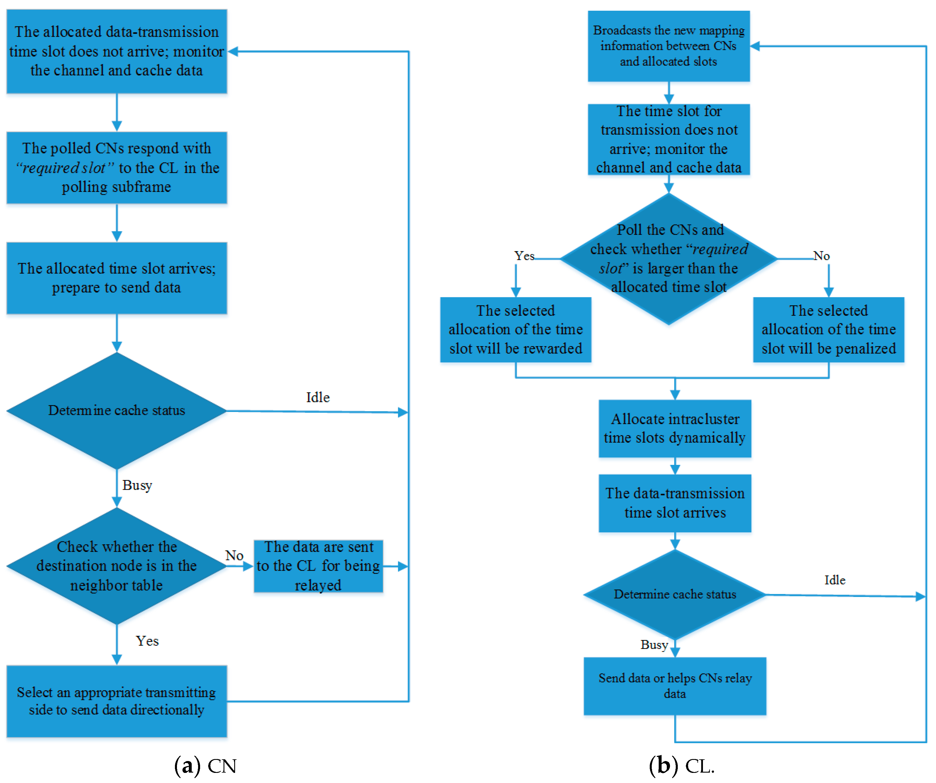
Working process

Figure 5 shows the communication flow diagrams of the CN and CL under the CL-LA MAC protocol. When the allocated data transmission time slot does not arrive, the CN keeps monitoring the channel and stores the generated data. The polled CNs respond with “required slot” to the CL in the polling subframe. When the allocated time slot arrives, the cache state is determined. If it is (i) BUSY, there are data in the cache queue, and it should be checked whether the destination node is in the neighbor table. If it is there, an appropriate transmitting side should be selected for sending the data according to the table; otherwise, the data are transmitted to the CL to be forwarded. If the cache state is (ii) IDLE, the cache queue is idle, and the node continues monitoring channels and storing data.

The CL broadcasts mapping information between the CNs and their allocated slots at the frame header. The CL stores the forwarded data from the CNs and their own generated data when the data transmission time slot does not arrive. In the polling subframe, the CL completes the dynamic allocation of the intracluster time slots according to the polling results. When the data transmission time slot arrives, the CL starts to send its own data or forward the data of the CNs.

4. Stable Cache Probability Distributions Based on MC

A.

Cache-queuing model

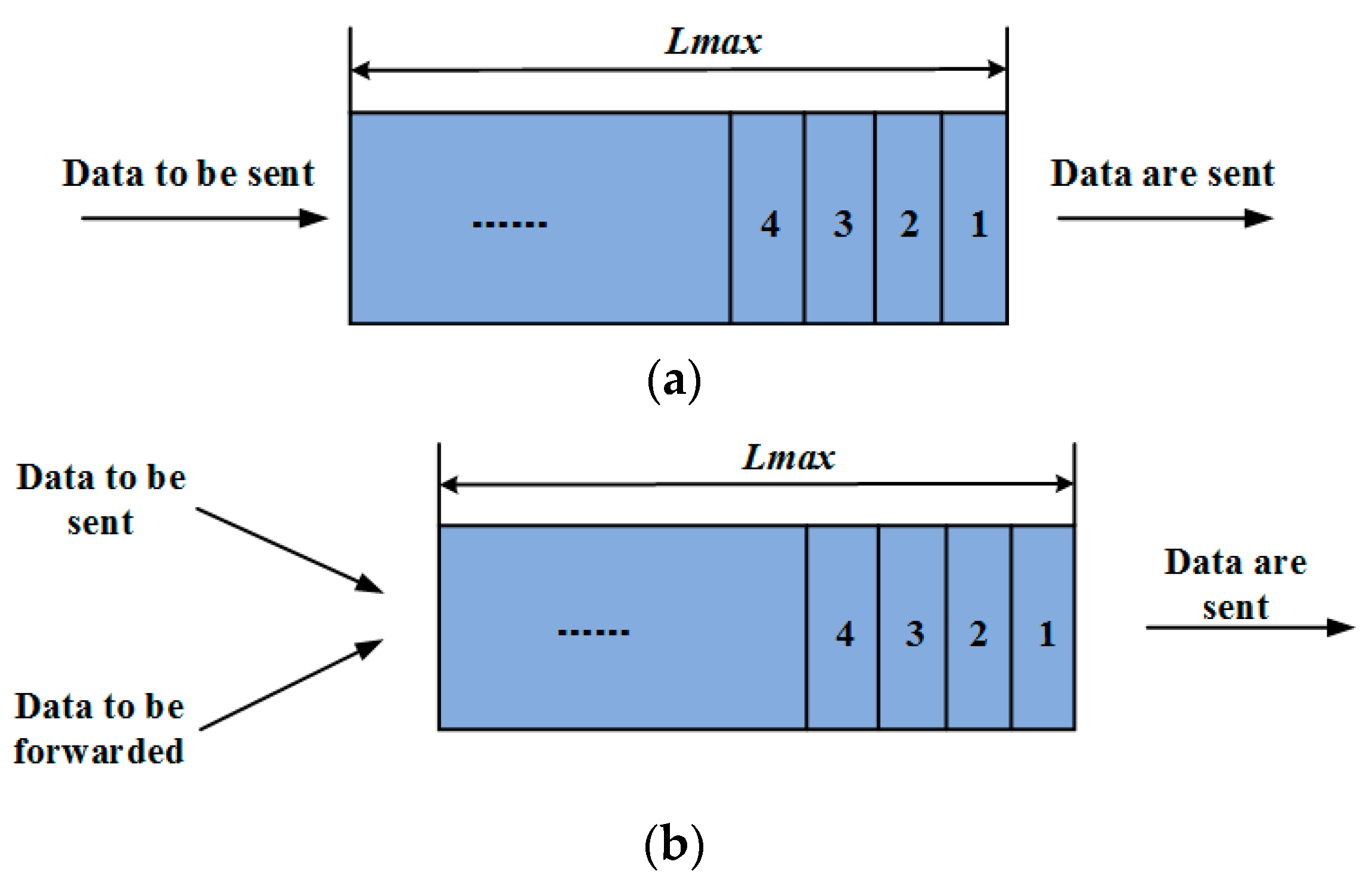
Figure 6 shows the cache-queuing model of the CN and CL. The generated data enter the cache in sequence. When the data transmission time slot arrives, the node sends the data based on the first in, first out (FIFO) method. The data class in the CN cache is different from that of the CL, including the forwarded data generated by the CN. The network performance could be analyzed iteratively since the cache lengths of the CL and CN followed state-dependent queuing models.

B.

Cache queue length

The arrival of data at each node in the network obeyed the Poisson process. Let p_x(x) and p_y(y) be the probabilities of the x-forwarded and y-non-forwarded data reaching, and they were subjected to the Poisson processes with intensities λ_x and λ_y, respectively.

$$p_x(x)=\frac{e^{-{\lambda }_{x}E}{\left({\lambda }_{x}E\right)}^x}{x!};$$

(3)

$$p_y(y)=\frac{e^{-{\lambda }_{y}E}{\left({\lambda }_{y}E\right)}^y}{y!},$$

(4)

where E is the unit time slot.

The sum of the data reaching probabilities is given by:

$$p_z(z)=\frac{e^{-{\lambda }_{\mathrm{z}}E}{\left({\lambda }_{\mathrm{z}}E\right)}^z}{z!},$$

(5)

where λ_z = λ_x + λ_y.

The probability of forwarded data is:

$$p_1=1-p_x(0).$$

(6)

If each cluster has M nodes, the probability of m nodes producing the forwarded data is:

$$p_2(m)=C_M^m{p_1}^m{(1-p_1)}^{M-m}.$$

(7)

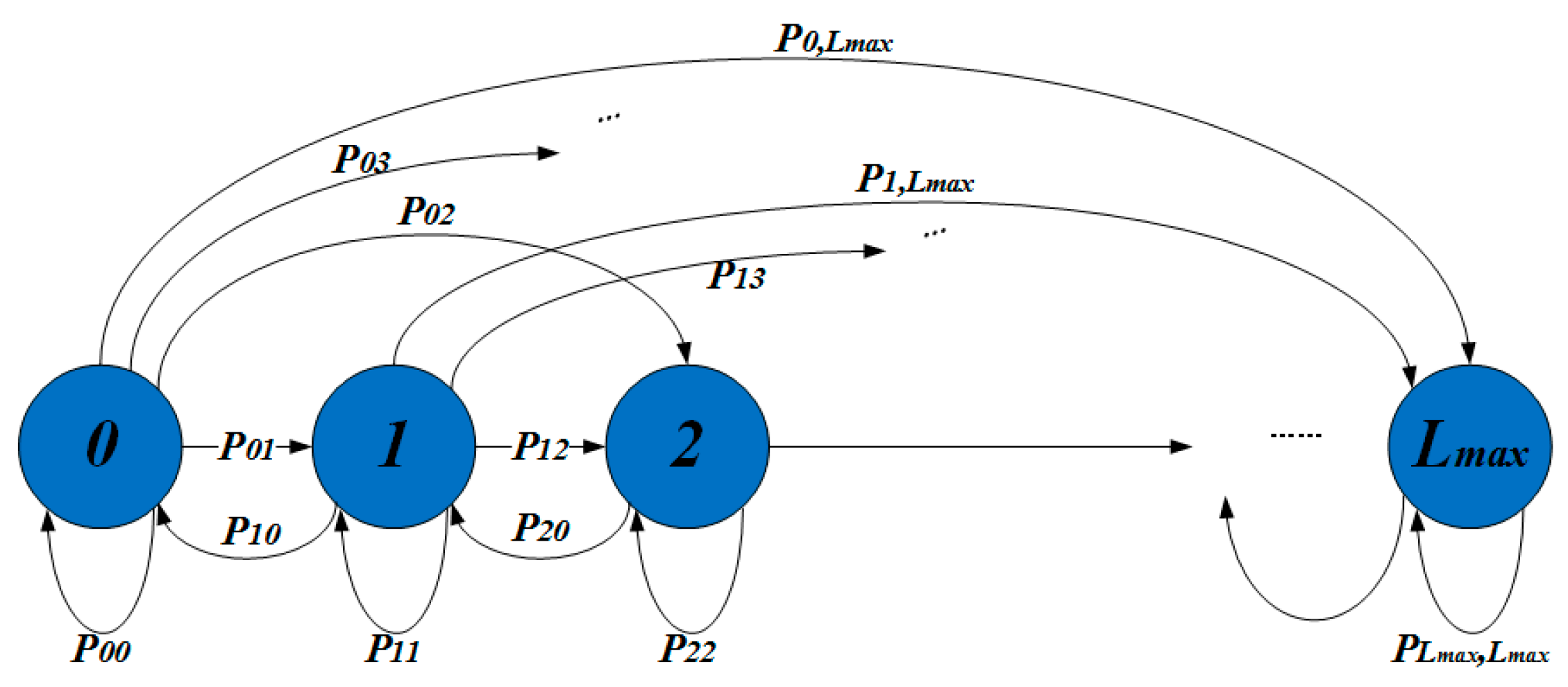
After unit time t, the cache length of the node becomes L_t. The cache length of the node at this moment only depends on the cache length at the previous moment, and the data packet changes at the current moment.

$$\begin{array}{c}P\left(L_t=l_t| L_1=l_1,L_2=l_2,\dots ,L_{t-1}=l_{t-1}\right)\\ =P\left(L_t=l_t| L_{t-1}=l_{t-1}\right).\end{array}$$

(8)

Therefore, the cache change is a Markov process. Figure 7 illustrates the Markov state transition diagram.

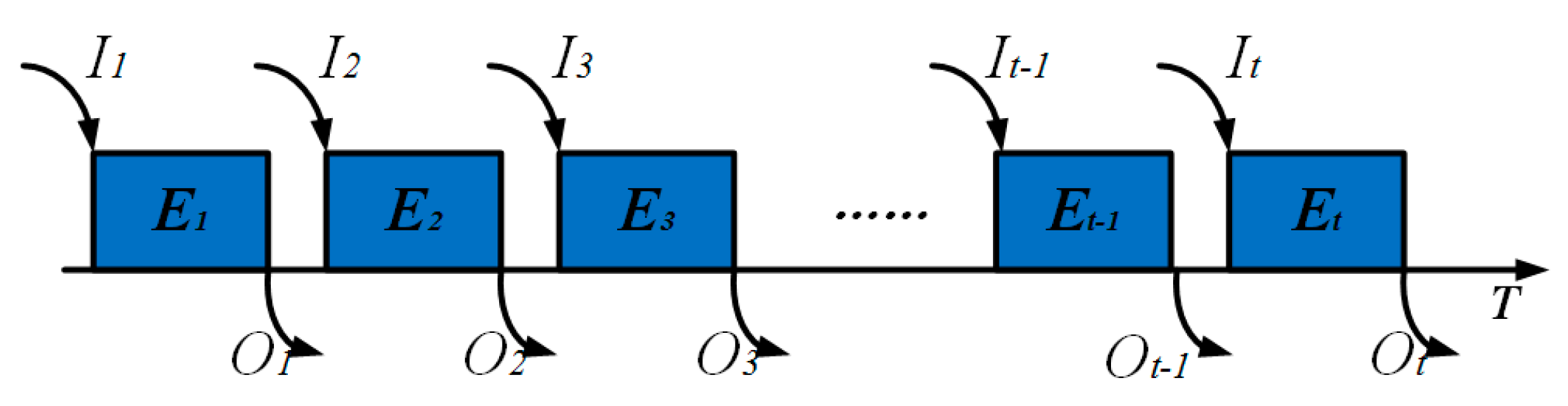
The transfer process of the cache length is shown in Figure 8, where I_t is the number of packets reaching at the time E_t⁻, and O_t is the number of data packets transmitted at E_t⁺. The node only sends data in the allocated time slot, thus, O_t can be either “0” or “1”.

Let $P_{ab}=P\left\{L_{t+1}=b| L_t=a\right\}$ be the probability that the state of the cache a at time t transfers to the state of the cache b at next unit time.

Based on Figure 8,

$$L_{t+1}=\left\{\begin{array}{ll}{L}_t+I_{t+1}-O_t\hfill & E_t\ge 1\hfill \\ I_{t+1}\hfill & E_t=0\hfill \end{array}\right.,$$

(9)

$$P_{ab}=\left\{\begin{array}{l}P\left\{L_{t+1}=b| L_t=0\right\}\\ =P\left\{I_{t+1}=b\right\}a=0,0\le b<L_{\max }\\ P\left\{L_{t+1}=L_{\max }| L_t=0\right\}\\ =P\left\{I_{t+1}\ge L_{\max }\right\}a=0,b=L_{\max }\\ P\left\{L_{t+1}=b| L_t=a\right\}\\ =P\left\{I_{t+1}-O_t=b-a\right\}1\le a<L_{\max },0\le b<L_{\max }\\ P\left\{L_{t+1}=L_{\max }| L_t=a\right\}\\ =P\left\{I_{t+1}-O_t\ge L_{\max }-a\right\}1\le a<L_{\max },b=L_{\max }\end{array}\right..$$

(10)

The transition matrices T of the two classes of nodes are obtained as follows (see Appendix A for the derivation process):

$$T^{CN}=\left[\begin{array}{cccccccc}{P}_{00}^{CN}& P_{01}^{CN}& P_{02}^{CN}& \cdots & \cdots & \cdots & P_{0L_{\max }-1}^{CN}& 1-{\displaystyle \sum _{i=0}^{L_{\max }-1}{P}_{0i}^{CN}}\\ P_{10}^{CN}& P_{11}^{CN}& P_{12}^{CN}& P_{13}^{CN}& \cdots & \cdots & P_{1L_{\max }-1}^{CN}& 1-{\displaystyle \sum _{i=0}^{L_{\max }-1}{P}_{1i}^{CN}}\\ 0& P_{21}^{CN}& P_{22}^{CN}& P_{23}^{CN}& P_{24}^{CN}& \cdots & P_{2L_{\max }-1}^{CN}& 1-{\displaystyle \sum _{i=1}^{L_{\max }-1}{P}_{2i}^{CN}}\\ \cdots & \cdots & \cdots & \cdots & \cdots & \cdots & \cdots & ⋮\\ 0& \cdots & \cdots & \cdots & \cdots & 0& P_{L_{\max }{L}_{\max }-1}^{CN}& 1-P_{L_{\max }{L}_{\max }-1}^{CN}\end{array}\right],$$

(11)

$$T^{CL}=\left[\begin{array}{cccccccc}{P}_{00}^{CL}& P_{01}^{CL}& P_{02}^{CL}& \cdots & \cdots & \cdots & P_{0L_{\max }-1}^{CL}& 1-{\displaystyle \sum _{i=0}^{L_{\max }-1}{P}_{0i}^{CL}}\\ P_{10}^{CL}& P_{11}^{CL}& P_{12}^{CL}& P_{13}^{CL}& \cdots & \cdots & P_{1L_{\max }-1}^{CL}& 1-{\displaystyle \sum _{i=0}^{L_{\max }-1}{P}_{1i}^{CL}}\\ 0& P_{21}^{CL}& P_{22}^{CL}& P_{23}^{CL}& P_{24}^{CL}& \cdots & P_{2L_{\max }-1}^{CL}& 1-{\displaystyle \sum _{i=1}^{L_{\max }-1}{P}_{2i}^{CL}}\\ \cdots & \cdots & \cdots & \cdots & \cdots & \cdots & \cdots & ⋮\\ 0& \cdots & \cdots & \cdots & \cdots & 0& P_{L_{\max }{L}_{\max }-1}^{CL}& 1-P_{L_{\max }{L}_{\max }-1}^{CL}\end{array}\right].$$

(12)

First, the cache probability distributions of the two classes of nodes is:

$$\left\{\begin{array}{l}{\partial }^{CN}(0)=\left({\partial }_0^{CN}(0),{\partial }_1^{CN}(0),\cdots {\partial }_{L_{\max }}^{CN}(0)\right)\\ =(1,0,0,\cdots 0)\\ {\partial }^{CL}(0)=\left({\partial }_0^{CL}(0),{\partial }_1^{CL}(0),\cdots {\partial }_{L_{\max }}^{CL}(0)\right)\\ =(1,0,0,\cdots 0)\end{array}\right..$$

(13)

After unit time t, the cache probability distributions of the two classes of nodes is:

$$\left\{\begin{array}{l}{\partial }^{CN}(t)=\left({\partial }_0^{CN}(t),{\partial }_1^{CN}(t),\cdots {\partial }_{L_{\max }}^{CN}(t)\right)\\ =\left({\partial }_0(0),{\partial }_1(0),\cdots {\partial }_{L_{\max }}(0)\right)\cdot {\left(T^{CN}\right)}^t\\ {\partial }^{CL}(t)=\left({\partial }_0^{CL}(t),{\partial }_1^{CL}(t),\cdots {\partial }_{L_{\max }}^{CL}(t)\right)\\ =\left({\partial }_0(0),{\partial }_1(0),\cdots {\partial }_{L_{\max }}(0)\right)\cdot {\left(T^{CL}\right)}^t\end{array}\right..$$

(14)

Because the cache change follows a recurrent finite Markov process, there are stable states. The sum of the cache probability distribution is one, which is expressed as:

$$\left\{\begin{array}{l}\underset{t\to \infty }{\lim }{\displaystyle \sum _{i=0}^{L_{\max }}{\partial }^{CN}(t)}=1\\ \underset{t\to \infty }{\lim }{\displaystyle \sum _{i=0}^{L_{\max }}{\partial }^{CL}(t)}=1\end{array}\right..$$

(15)

Therefore, the stable cache probability distributions of the CL and CN could be obtained iteratively.

5. Simulation and Analysis

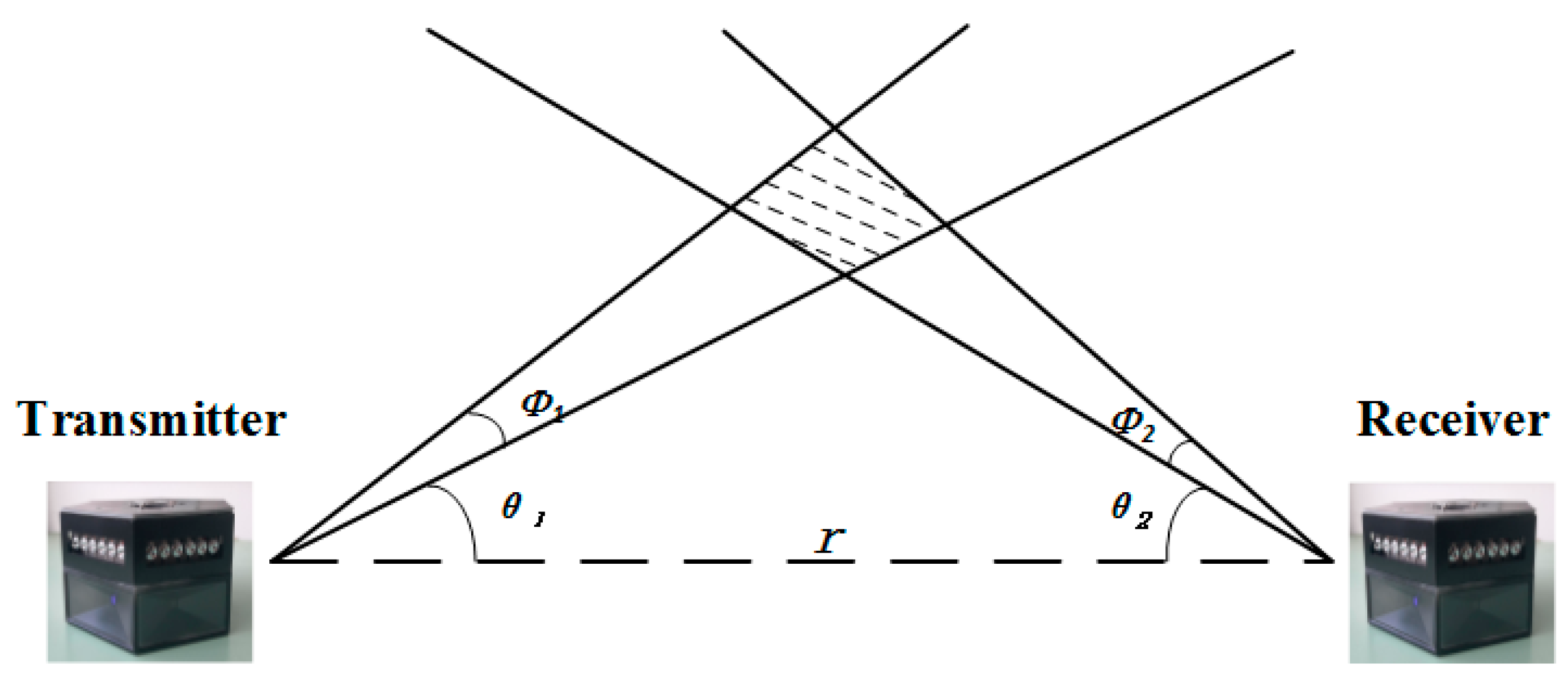
Figure 9 illustrates the UV NLOS communication model. According to our previous study [23], the communication distance of a UV terminal, according to the on–off keying (OOK) modulation, is given by:

$$R_{OOK}=\sqrt[\alpha ]{-\frac{\eta \lambda P_t}{hc\xi R_b\ln \left(2P_e\right)}},$$

(16)

In the simulation, the communication radii of the CL and CN were 210 and 60 m, which was consistent with the lengths of the radii in the actual situation of our previous experiments [24].

The classes of service were classified into forwarded and non-forwarded data. Let the proportion of non-forwarded data to the total data (p_non) denote network scenarios with different classes of service. With the development of UV light sources, photoelectric detection techniques, and modulation coding modes, much higher rates than several Mbps are achieved in the UV point-to-point communication system [25]. However, the UV networks are primarily limited by the networking method, topology control, and terminal movement, and the actual working rate can only be limited to below 100 kbps [26]. To ensure the reliable transmission of information, the data rate is selected as 50 kbps in the simulations of the multi-node UV network. The simulation parameters are shown in

Table 1. Simulation Parameters.

Parameter	Value
UV terminals	24
communication distance of CL dCL	210 m
communication distance of CN dCN	60 m
data rate Rb	50 kbps
packet length L	500 bit
time slot length σ	10 ms
cache of CL	3
cache of CN	3
simulation time	500 s

.

A.

Network topology

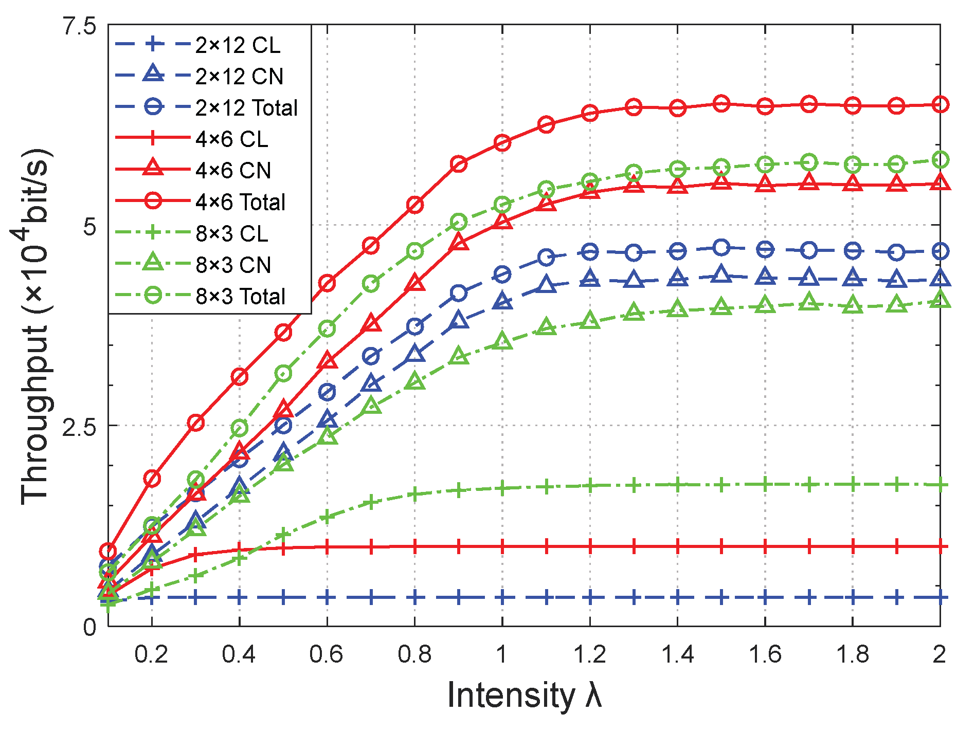
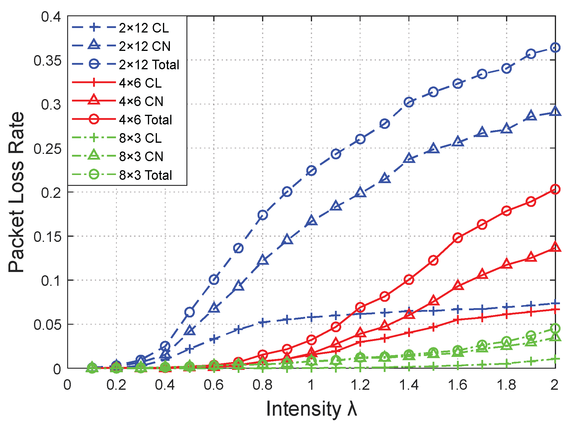
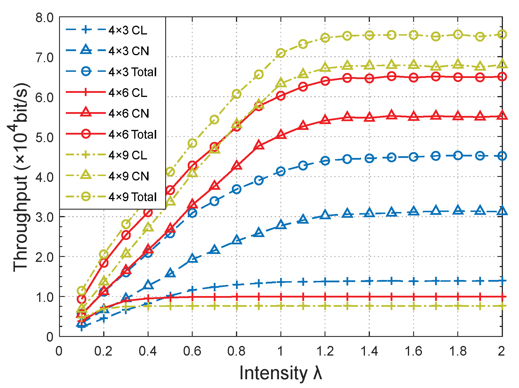
Figure 10 and Figure 11 show the relationship between network performances and data arrival intensity λ with different network topologies, respectively. The topology structure is expressed as A × B, representing A × CLs in the topology and B × CNs in each cluster. The p_non was 0.6.

The network performances versus λ were approximately identical for different network topologies. First, the intensity λ increased, increasing the throughput. With the continuous increase of λ, each time slot in the network is gradually occupied, and the channel tends to be saturated. Even if the λ increases, the network throughput cannot increase and remains constant. Moreover, there will be an upper bound on the throughput, which is related to the network topology. Meanwhile, the increasing amount of data led to an overflow in the terminal cache and a gradual increase in the packet loss rate.

The throughput of the CL was lower than that of the CN since the forwarded packet occupied the data transmission time slot of the CL, as shown in Figure 10. When the network topology changed from 2 × 12 to 4 × 6, the throughput ratio of the CL to CN data increased from 8.25% to 17.87%, while it increased to 46.30% in the 8 × 3 topology when the λ was 1.20.

Compared to the throughputs in the 4 × 6 (0.99 × 10⁴ bit/s) and 2 × 12 (0.36 × 10⁴ bit/s) topologies when the intensity λ was 1.20, the throughput of the CL was the highest (1.75 × 10⁴ bit/s) in the 8 × 3 topology, owing to the highest number of CLs being set in these simulations. However, the throughput of the CN was the lowest (3.78 × 10⁴ bit/s) because there were only three CNs in each cluster and fewer services in the cluster. Additionally, the number of services was only 69.87% and 87.91% of that of the 4 × 6 (5.40 × 10⁴ bit/s) and 2 × 12 (4.30 × 10⁴ bit/s) topologies, respectively. The ratio of the CLs to CNs was relatively large, resulting in the burden of each CL being reduced and the packet loss rate in the 8 × 3 topology network being the lowest, as shown in Figure 11. Inversely, there were a large number of CNs in each cluster of the 2 × 12 topology network, and the forwarded data caused an overflow at the cache of the corresponding CL. Therefore, the packet loss rate surged, making it significantly higher than that of the other two topologies.

The highest throughput (6.39 × 10⁴ bit/s) and acceptable packet loss rate (approximately 8%) of the 4 × 6 topology was achieved when λ was 1.2, owing to the relative appropriateness of the topology setup. Therefore, the network topology should be reasonably set to achieve a better performance in the actual networking.

B.

Class of service

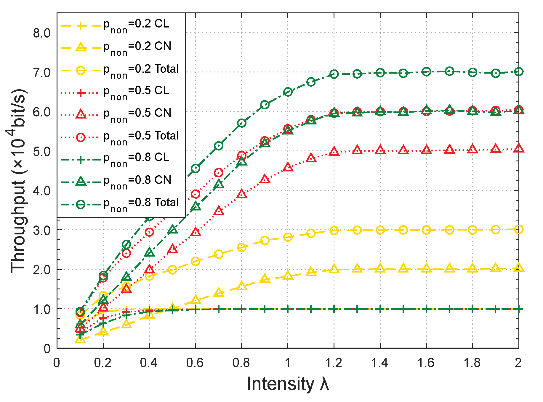
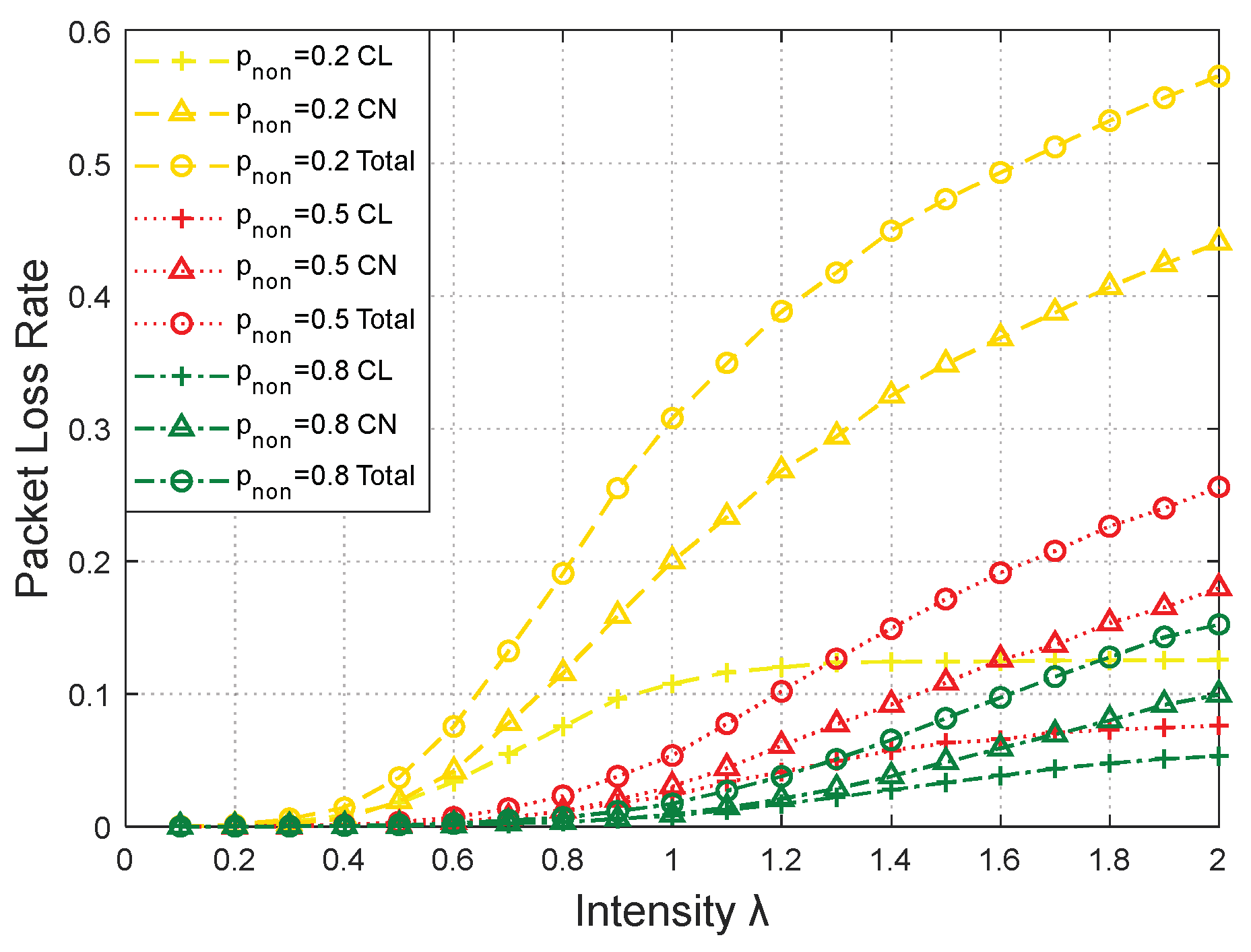
Figure 12 and Figure 13 illustrate the relationship between network performances and data arrival intensity λ with various classes of service (p_non = 0.2, 0.5, and 0.8). The network topology was 4 × 6.

When p_non was larger, more data packets could be directly transmitted within the cluster, resulting in better performances. Figure 12 and Figure 13 show that the total throughput with p_non = 0.5 increased by approximately 99.66% from 2.98 × 10⁴ to 5.95 × 10⁴ bit/s, compared to the total throughput with p_non = 0.2. Additionally, the corresponding packet loss rate decreased by 74.36% from 0.39 to 0.10 when the intensity λ was 1.20. This rate of increase in the throughput and decrease in the packet loss rate increased to 132.88% (from 2.98 × 10⁴ to 6.94 × 10⁴ bit/s) and 89.74% (from 0.39 to 0.04) from p_non = 0.2 to p_non = 0.8.

The number of CLs determined the maximum forward capacity in the CL-LA protocol. Therefore, the CL throughput rapidly overlapped for the three classes of service with the same number of CLs, as shown in Figure 12.

C.

Number of CNs

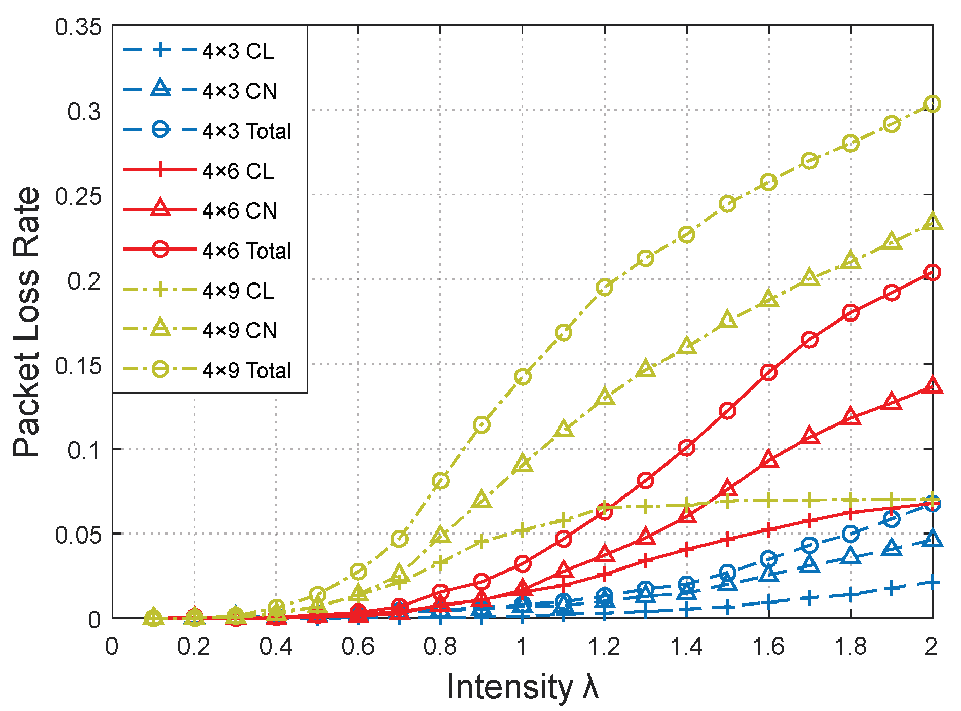
Figure 14 and Figure 15 illustrate the relationship between network performances and data arrival intensity λ with different numbers of CNs (i.e., 3, 6, and 9). The p_non was 0.6.

The network performances versus the intensity λ were approximately identical in relation to the network performance regarding the number of CNs. A network with more CNs produced more packets with the same number of CLs, resulting in better performances.

Figure 14 shows that the throughput of a CL with nine CNs was the lowest (0.76 × 10⁴ bit/s), which was only 76.66% and 55.47% of that with six (0.99 × 10⁴ bit/s) and three CNs (1.37 × 10⁴ bit/s), respectively, when λ was 1.20. As the number of CNs increases, more forwarded data were generated with the same p_non, and more data transmission time slots of the CLs are occupied by forwarded packets, leading to a decrease in the throughput of the CL. More forwarded packets were crowded and overflowed at the corresponding CLs, leading to a sharp increase in the packet loss rate, as shown in Figure 15.

Although increasing the number of CN nodes could increase the network throughput to a certain extent, the packet loss rate would sharply increase, and the network performance would deteriorate due to an increase in the services outside the cluster. Therefore, the topology of the network structure must be reasonably set and the number of clusters must be adjusted accordingly.

D.

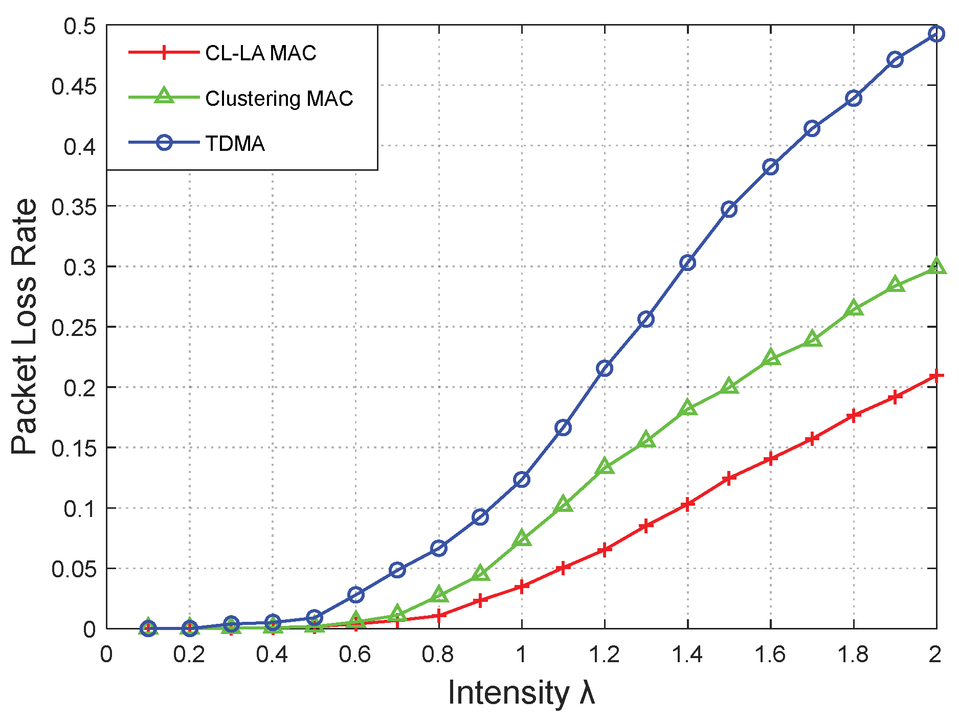
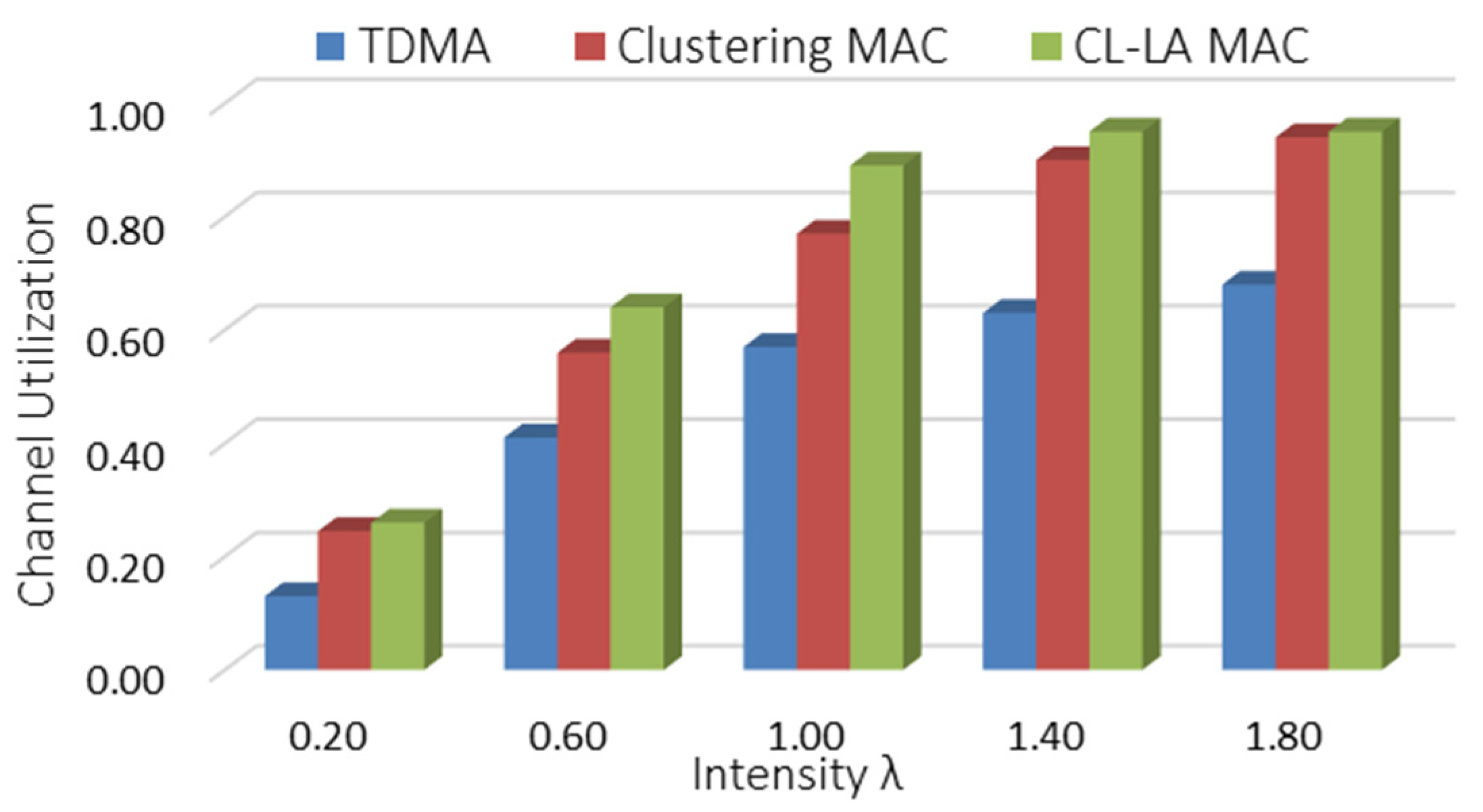
Comparison with TDMA and clustering MAC protocols

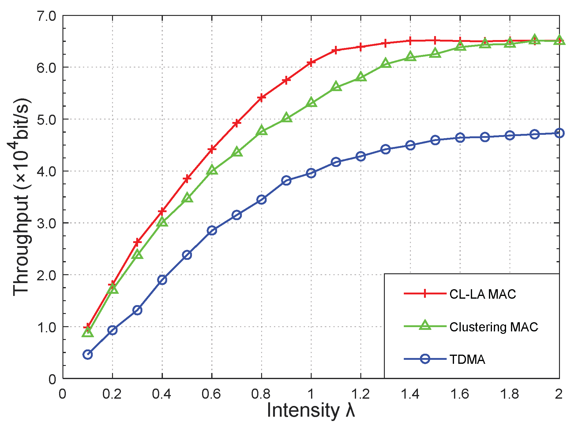
Figure 16, Figure 17 and Figure 18 show the comparison of the network performances for the three MAC protocols. The network topology was 4 × 6, and the p_non was 0.6.

Horizontally comparing the results from the three MAC protocols in Figure 16 and Figure 17 show that the network performance of the clustering mechanism was significantly higher than that of the TDMA protocol. Compared with the clustering protocol, the CL-LA protocol had a higher throughput (increased by approximately 14.91% when λ = 1.00) and lower packet loss rate (decreased by 53.42%) due to the application of the LA algorithm.

Figure 18 shows the channel utilization for three MAC protocols. The data transmission time slot could be dynamically allocated under the CL-LA protocol when the data arrival of each node was unbalanced, causing the upper bound of the throughput to be rapidly reached and the channel resources to be fully utilized.

6. Discussion

At present, the UV protocols are relatively lacking, especially in multi-node networks [5,7]. For application in large-scale UV node networking, this study improves the conventional TDMA protocol based on the clustering topology and LA algorithm. The simulation results reveals that the CL-LA MAC protocol obtains a better network performance, proving its suitability for multi-node UV networking.

The overhead of the RL algorithm is added to the frame structure to achieve dynamic time slot allocation and fully utilize the channel. The complexity of the system does increase but still within acceptable limits. Compared with other protocols that can achieve similar functions, the CL-LA protocol does not involve complex handshake mechanisms, simplifying its complexity. In addition, the performance of the proposed protocol is better than the conventional ones [27]. The CL-LA MAC protocol provides practical guidance for the development of UV multi-node networking.

As the cluster head, the CL had to frequently send important control data. However, because the FIFO method was adopted in the current CL-LA mechanism, forwarded packets from the CNs frequently occupied the data transmission time slot of the CL, resulting in a loss in the packet overflow and a low throughput for the CL, owing to the limited cache. Therefore, in the future, we aim to configurate various caches to classes of service or set a higher priority for the CL data to guarantee the transmission of control data.

7. Conclusions

A CL-LA MAC protocol based on the clustering topology and LA algorithm was proposed. We thoroughly described the LA algorithm and communication flow. Moreover, the stable cache probability distributions of CN and CL were separately derived based on the MC. To obtain the most suitable network performance, the effects of network topology, class of service, and number of CNs on the network performance under the novel CL-LA MAC protocol were analyzed, and the structural parameters were optimized. In the simulation, the performances of the CL and CN were examined separately to perform a more detailed and intuitive analysis. Compared with the TDMA and clustering system, the CL-LA protocol achieved a higher throughput and channel utilization and a lower packet loss rate, owing to the clustering mechanism and dynamic time slot allocation, fully proving the effectiveness of the proposed protocol. The CL-LA MAC protocol is a novel, reliable, and effective method for multi-node UV networking.