1. Introduction
Coherence scanning interferometry (CSI) is a widely used technique for areal surface topography measurement [
1]. The International Organization for Standardization (ISO) recommends employing the ‘W/3 rule’ for calculating the groove depth of rectangular gratings [
2]. However, the batwing effect, characterized by an overshoot at the edges of the grooves, can have a significant impact on the accuracy of depth measurements [
3,
4]. Importantly, as the period of the rectangular grating decreases, the batwing extends beyond the region of W/3 near the edge of the groove [
5], leading to significant errors in depth measurement for small grating periods. Therefore, it is necessary to establish and analyze the relationship between batwing and depth measurement errors. The overshoot profiles of the batwing are influenced by various factors, such as the center wavelength, spectrum of the illuminating light, shadow effect, and numerical aperture (NA). The above can be quantitatively analyzed to identify the dominant factor that affects depth measurement errors. This paper specifically examines grating depths smaller than the coherence length of the illuminating light, as the batwings cease to appear beyond certain depths [
4].
Modeling is an effective approach for investigating correlations between key factors and measurement outcomes. Many previous works have established models to investigate these relationships. Peter De Groot devised a computationally efficient theoretical model that analyzed the relationship between the illumination geometry, the spectrum of the illuminating light and the interference signals [
6]. Additionally, He established an elementary Fourier optics model to analyze the relationship between surface and main features of CSI topography images [
7]. Harasaki developed a diffraction model elucidating the relationship between the coherence length of the illuminating light and the batwing effect [
4]. Xie proposed a Fourier model for analyzing the relationship between the lateral resolution and the transfer function of vertical scanning white-light interferometers [
8,
9]. Tobias presented a 3D simulation model investigating the transfer characteristics of confocal microscopes regarding 2D surface structures [
10]. Su proposed a physics-based virtual CSI based on the foil model and obtained an inverse filtering is shown to reduce measurement errors [
11,
12]. Peter Lehmann suggested that the three-dimensional transfer function of the CSI is crucial for the correct analysis and reconstruction of the surface of the object [
13]. Although the aforementioned works explain the correlation between main factors and measured topography, and some have addressed the impact of the batwing effect on step height measurements as well as the elimination of this effect in reconstructed morphology [
14,
15], none specifically investigate the relationship between the batwing effect and measurement error when utilizing the ‘W/3 rule’ for depth calculation.
The batwing is usually taken as a pseudo signal, and it is directly filtered or the topography where the batwing occurred is directly ignored. But whether the batwing effect will affect the depth calculation is still unknown, even if the overshot on the topography seems like to be filtered out. It is evident that batwings within the selected W/3 region intuitively influence depth measurement errors, but the exact relationships remain indirect. In this paper, we present a method that aims to determine the height and width of the batwing. Additionally, we seek to establish the correlation between the batwing effect and the errors encountered in depth measurements. Additionally, a simulation model is proposed and utilized to analyze these correlation relationships, ultimately identifying the primary factors that contribute to errors in measuring the grating depth.
2. Definitions and Models
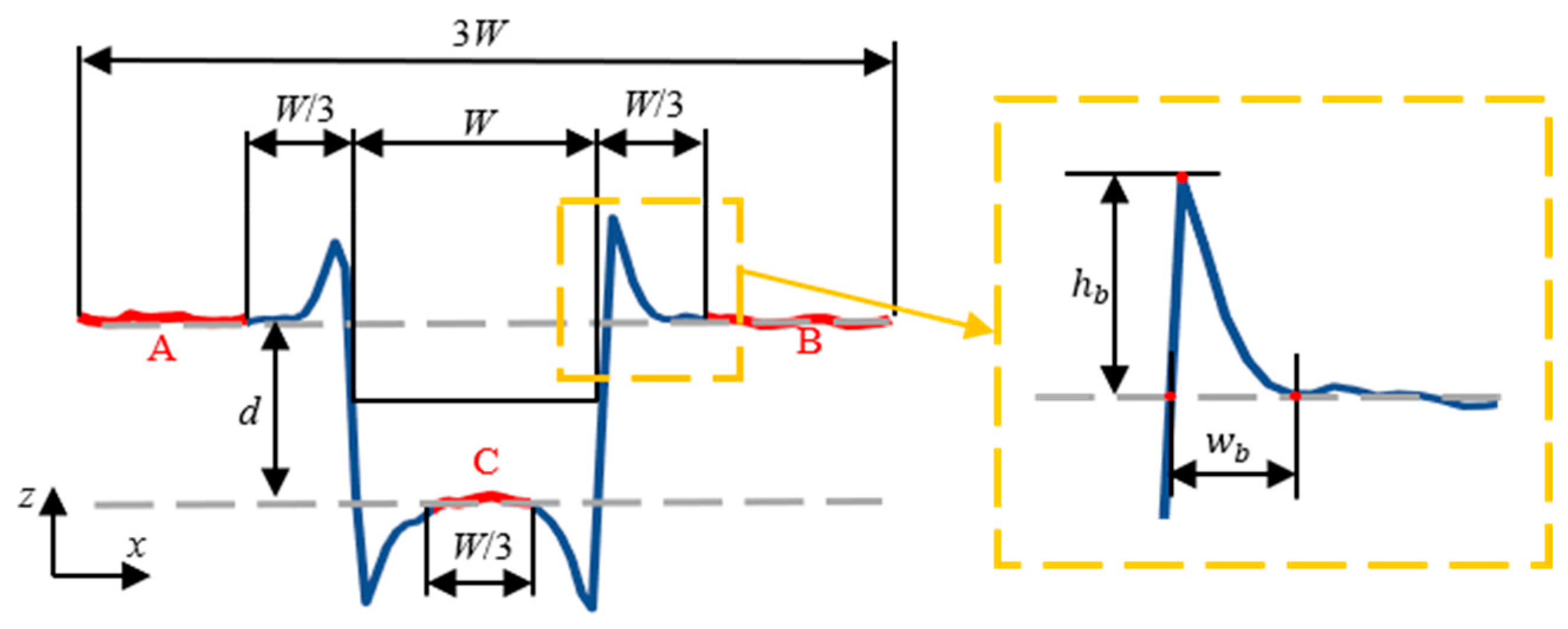
Figure 1 illustrates the ‘W/3 rule’ and provides definitions for the batwing height and width. In this figure, W represents the measured width of the groove. Least square lines are fitted to regions A and B, and subsequently to region C [
2].
The groove depth
d is determined by the distance between the fitted lines.
where
,
, and
h are fitted via the least squares method to a profile. The variable
δ takes the value +1 in regions A and B and the value −1 in region C. The depth of the groove
d is twice the estimated value of
h.
The batwing height
is defined as the difference in height between the highest point on the batwing profile and the fitted line.
where
represents the coordinates of the highest point on the batwing profile. The batwing width
is defined as the distance between the two intersection points of the batwing profile and the fitted line, with these points being the closest intersections on either side of the batwing.
where
and
are the two intersection points of the batwing profile and the fitted line.
It is important to note that as the period of rectangular gratings decreases, the batwing extends beyond the W/3 region near the groove edge, affecting the accuracy of depth measurements in regions A, B, and C where least square lines are fitted. Additionally, the batwing width and height vary depending on the parameters of the microstructures being tested and the specifications of the CSI instrument. Therefore, it is necessary to analyze the influence of the batwing effect on groove depth measurements of rectangular gratings using CSI and the ‘W/3 rule’. Establishing a model provides an effective and quantitative approach to understand the relationship between influencing factors and depth measurement errors.
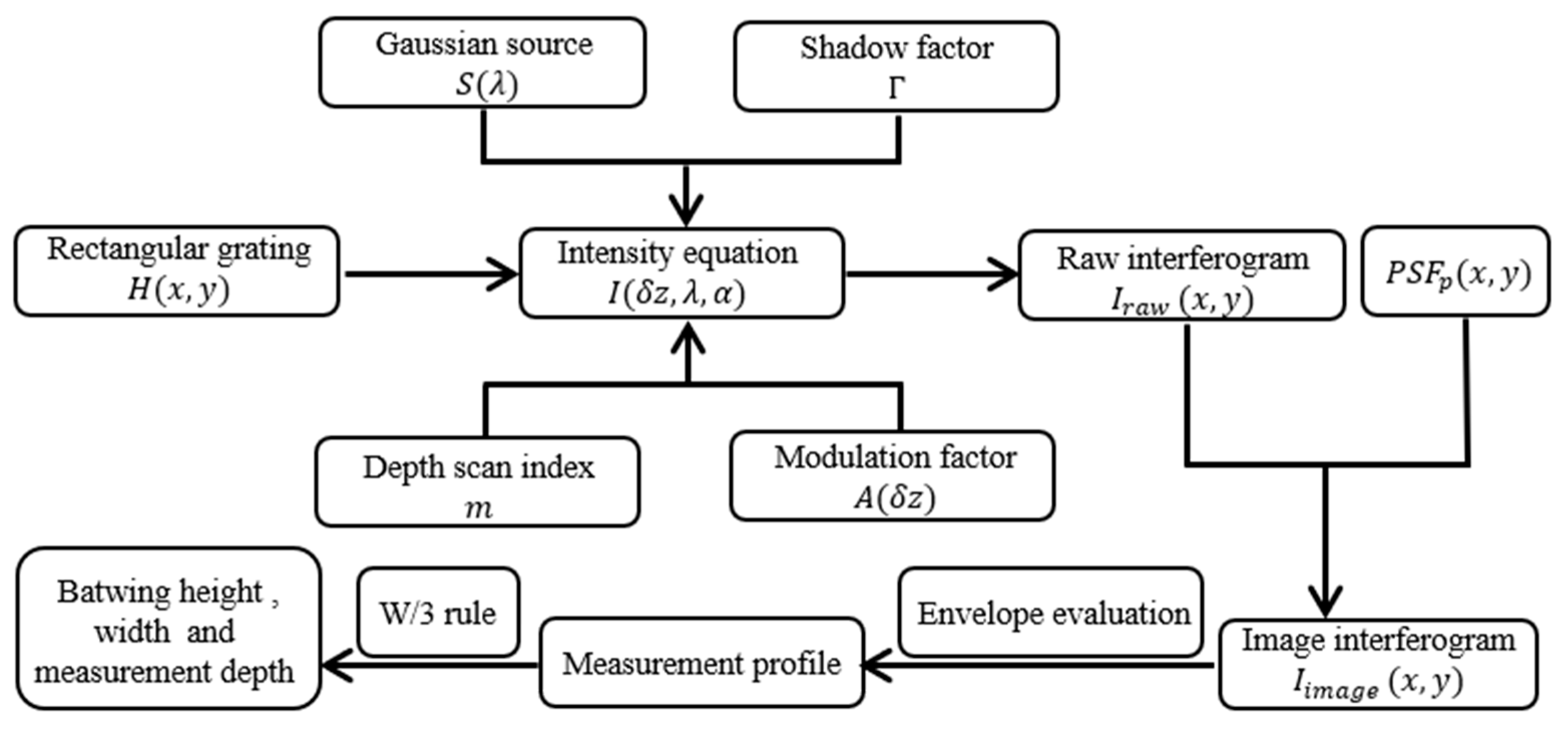
The simulation process is depicted in
Figure 2. Initially, the nominal period and depth of the rectangular grating are provided as inputs. Subsequently, the depth scan index, modulation factor, illumination spectrum, and shadow factor are combined using the interference intensity equation to generate the corresponding interferograms. The envelope evaluation method is then employed to reconstruct the grating profile [
16]. Finally, the ‘W/3 rule’ is applied to calculate the depth of the rectangular grating and the height and width of the batwing from the measured profile.
The object taken in the simulation is a rectangular grating
with period Λ and groove depth
d [
8]. The illumination spectrum
is assumed to follow a Gaussian distribution [
17].
We assume that the depth of the grating is significantly smaller than the width of the coherent envelope, and that the power on the pupil plane is uniformly distributed. In contrast to Xie’s definition [
9], we define shadow factor Γ as the ratio of reflected power to incident power at the edge of the grating.
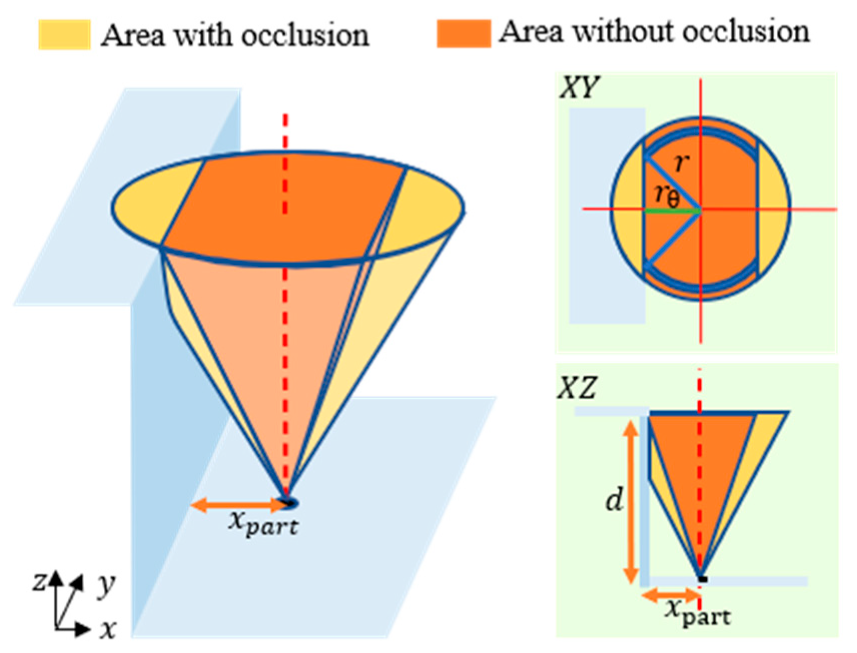
Figure 3 illustrates the shadow effect at the edge of the rectangular grating, which is expressed as:
with
where
represents the local coordinate of the grating bottom region,
represents the numerical aperture of the objective, and
represents the number of periods. The refractive index of air is approximately 1. This paper specifically focuses on grating depths that are significantly smaller than the depth of field. As a result, the influence of scanning depth on the shadow factor can be disregarded.
The modulation of the coherence signal is influenced by the temporal and spatial coherence, which are consequences of the illumination spectrum and the NA. The modulation factor is expressed as
where
is the scan step,
represents the depth of scan, and
m is the depth scan index.
A is used to characterize the modulation effect. With
where
σ represents the spatial coherence coefficient,
indicates spatial coherence, and
indicates coherence length of the illumination spectrum, respectively [
17]. According to Abdulhalim’s theory [
18], the simplified interference formula within this model from a planar object, denoted as
, represents the integration of the raw interferogram over the depth scan index, incident angles, and illumination spectrum. The raw interferogram does not take diffraction effects into account and is expressed as follows:
with
where
and
correspond to the longest and shortest wavelengths of the illumination spectrum, respectively.
To calculate the point spread function (PSF), we can utilize the analytical calculation method described by Goodman [
19], which involves performing a Fourier transform of the pupil function. In our approach, we use the focal plane PSF to approximate the out-of-focus PSF. For circular pupils, the
, after eliminating the constant factor, can be expressed as follows:
In this equation,
is the central wavelength,
x and
y represent coordinates on the planar object, and
J1 represents the Bessel function of the first kind and order one. As described by Abdulhalim [
17], when the grating depth is smaller than the coherence length, the maximum lateral coherence distance between two points in the object plane is
, as clarified in Equation (18). To reduce computational complexity, we focus our calculations on the intensity within the lateral coherence distance. This allows us to concentrate on the partial point spread function
(
x,
y), which can be formulated as follows:
According to Fourier optics, the diffraction effect can be expressed as follows:
where * represents the convolution operator.
(
x,
y) represents a series of stacked interferograms that consider the diffraction effect. The envelope method is applied to reconstruct the grating profile [
16]. Finally, the ‘W/3 rule’ is utilized to calculate the depth measurement of the rectangular grating.
It is worth noting that the boundaries of the simulation model are applicable to gratings with relatively low depths, which should be smaller than the center wavelength.
3. Simulations and Experiments
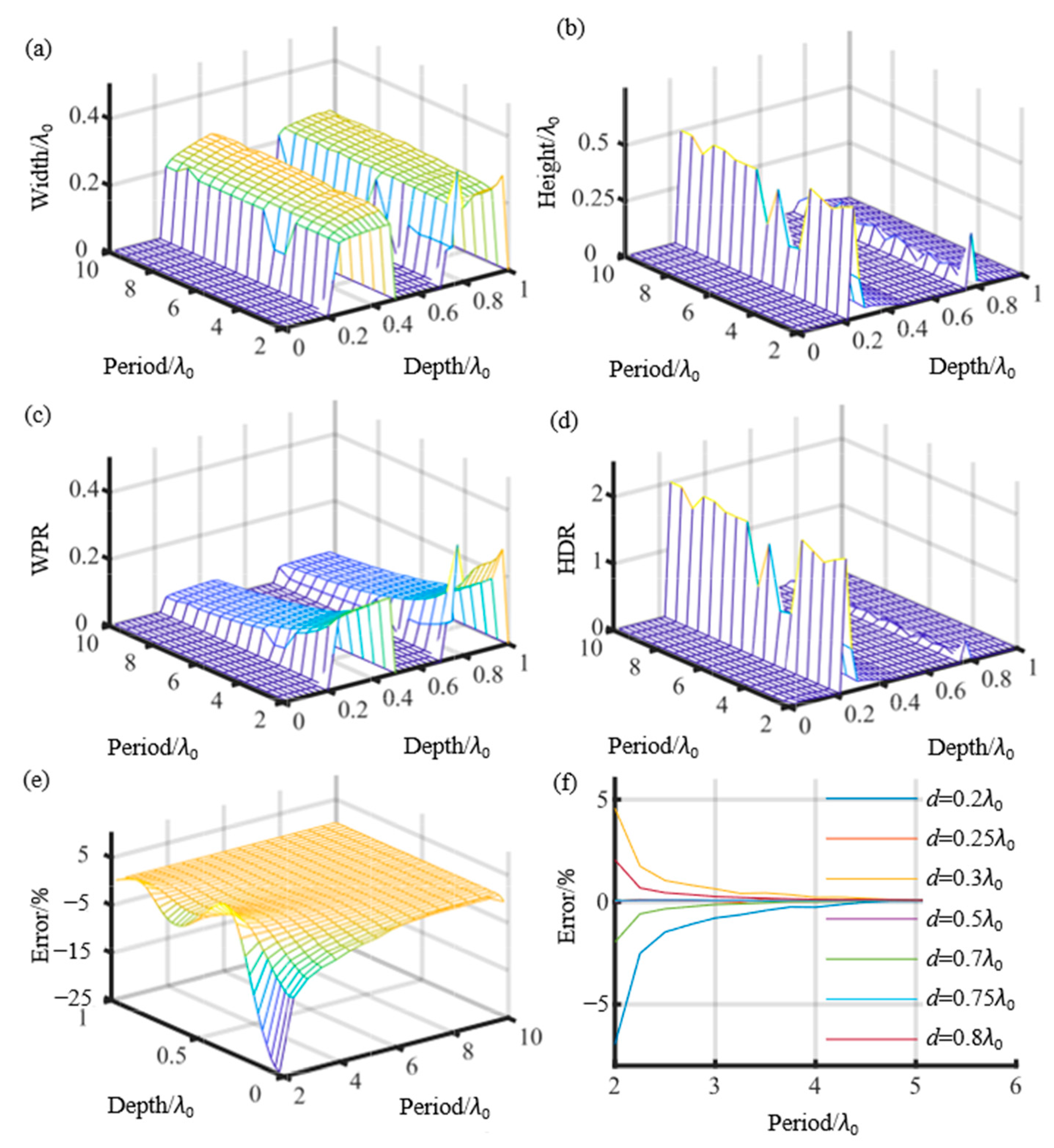
Figure 4a,b illustrate the batwing width and height values for different periods and depths of the grating. These figures also demonstrate the independence between batwing height and width.
Figure 4c illustrates the dominant influence of the width-to-period ratio (WPR) on depth measurement errors, which represents the ratio between the batwing width and the grating period. When the WPR is smaller than 1/6, the impact of the batwing on depth measurement errors can be disregarded.
Figure 4d shows the positive correlation between the height-to-depth ratio (HDR), which indicates the ratio between the batwing height and the grating depth, and depth measurement errors when the WPR values are similar and exceed 1/6.
Figure 4e,f display the depth measurement errors of rectangular gratings with different depths and periods, assessed using the envelope evaluation method [
16]. The depth measurement errors typically decrease as the grating period increases, except for certain instances near the depth values of
d = 0.25
λ0 and
d = 0.75
λ0. Grating depths smaller than or approximately equal to 0.25
λ0 (and also 0.75
λ0) result in negative depth measurement errors, whereas depths larger than or approximately equal to 0.25
λ0 (and also 0.75
λ0) yield positive errors [
20,
21,
22].
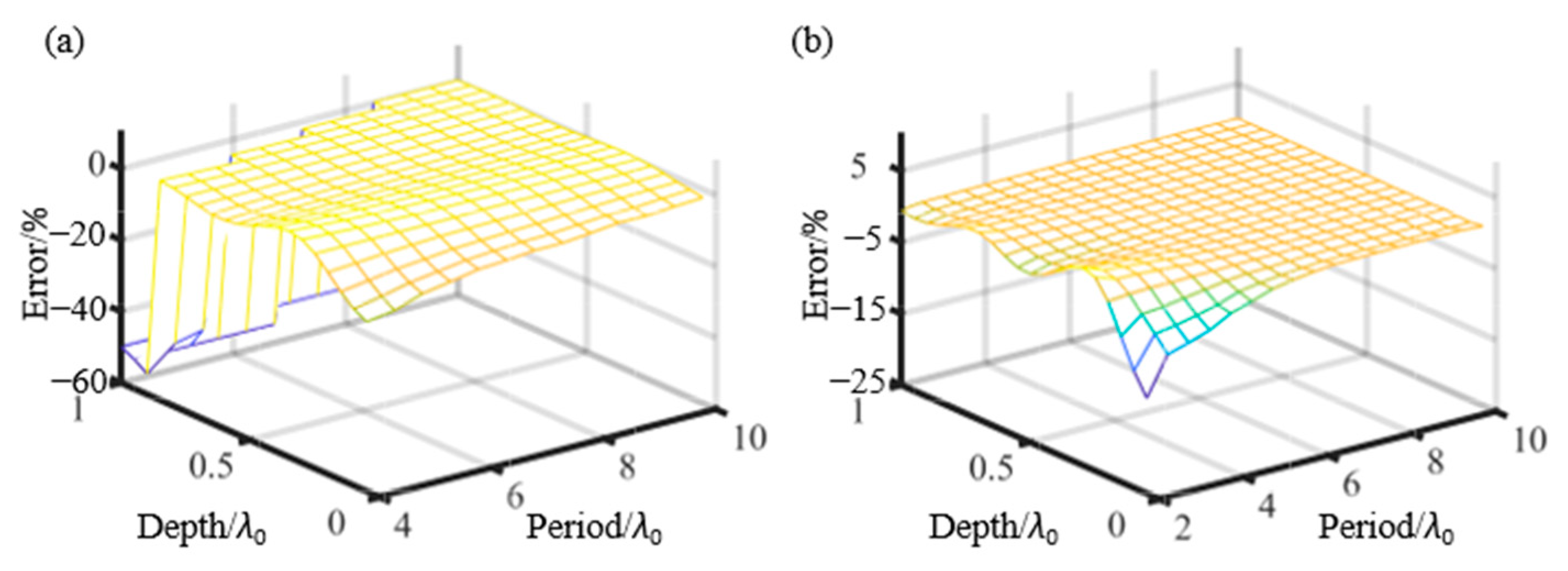
Figure 5a depicts the depth measurement errors with
AN = 0.3
λ0 = 0.6 μm. As the NA decreases, the batwing width increases, leading to large measurement errors for small grating periods, especially when the depth is close to
λ0. On the other hand,
Figure 5b shows the depth measurement errors with
AN = 0.55
= 0.5 μm. Decreasing the center wavelength leads to a reduction in the batwing width, resulting in smaller depth measurement errors for small grating periods. Moreover, we conducted simulations to examine the influence of altering the illumination spectrum and shadow factor on the depth measurement error, and we observed that these variations closely resemble the patterns depicted in
Figure 4e. Therefore, we can conclude that these factors have a minimal influence on the depth measurement error, and therefore, we have not included the corresponding figures in this paper.
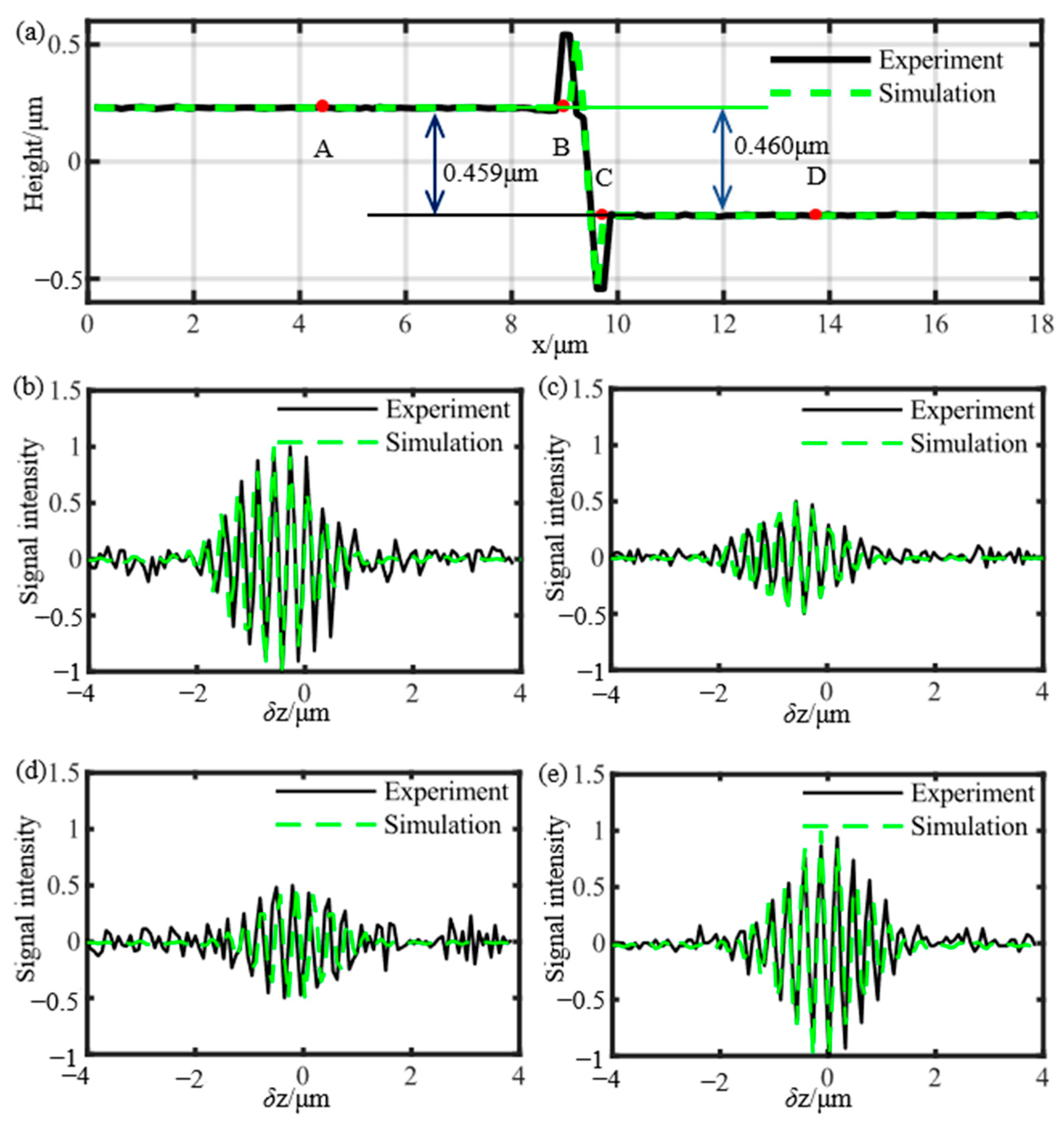
The Bruker step standard with a calibrated height of 0.4598 μm was measured using a Mirau objective with
AN = 0.55 and LED light sources with
λ0 = 0.6 μm and
= 0.08 μm.
Figure 6 presents a comparison between simulated and experimental results. In
Figure 6a, the black line represents the experimental profile, and the green line represents the simulated profile. In
Figure 6b–e, the black lines represent the experimental signals, and the green lines represent the simulated signals. These signals correspond to points A–D in
Figure 6a, respectively. We assumed
σ to be 0.5.
R1 and
R2 were constant and assumed to be 1.
Table 1 presents the values for
Figure 6a. The simulated and experimental results exhibit good agreement, as shown in
Figure 6a. The simulated values for batwing height and width are 0.3068 μm and 0.2530 μm, respectively. In comparison, the experimental values for batwing height and width are 0.3130 μm and 0.4987 μm, respectively.
The difference between simulated and experimental values for batwing width is probably due to the fact that the experimental standard step is quasi-perpendicular. Whether batwings appear or not depends not on the total groove depth but on the change of depth involved in the diffraction region [
21]. The simulated and experimental results for profile depth are 0.460 μm and 0.45934 μm, respectively. The relative errors with respect to the nominal value are 0.04% and −0.10%.
The comparison results between simulated and experimental envelope signals are presented in
Figure 6b–e, revealing a good match between the two sets of data. In
Figure 6c,d, the envelope of the signal exhibits asymmetry, which can be attributed to the presence of diffraction and shadow effect. A shadow effect occurs at the edge of the bottom region because the acceptance angle of the microscope objective is smaller than the maximal incident angle and that of the reflected rays passing through the optical system on the bottom [
21]. As shown in
Figure 3, the structure of the step standard prevents rays with high incident and reflected angles. And the signal at the edge of the top part is also influenced by the diffraction effect.
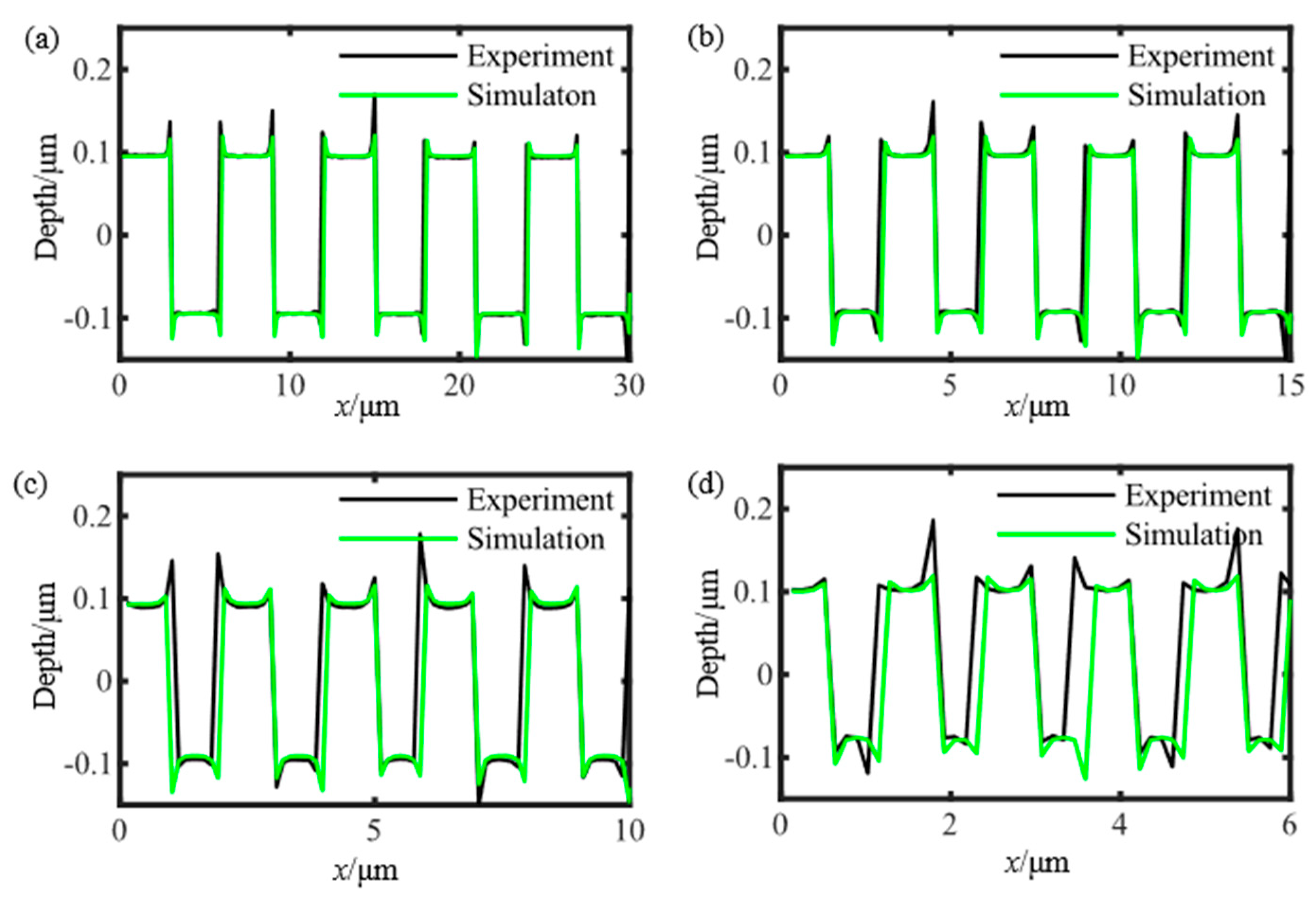
The resolution standard RS-N manufactured by Simetrics GmbH (Chemnitz, Germany) provides a set of rectangular gratings with different periods and depths. The periods range from 0.3 to 6 μm and the depths range from 0.1472 to 0.1896 μm. The standard was calibrated by the Metrological Large Range Scanning Probe Microscope (Met LR-AFM) based on the Nano Measuring Machine (NMM, GmbH, Wien, Germany) in the cleanroom centre of PTB (Physikalisch-Technische Bundesanstalt, Braunschweig, Germany) [
23].
As stated in ISO 25178-603, when the lateral resolution is limited by the lateral sampling interval of the image sensor system, the smallest period that can be measured should cover five pixels [
24]. However, for high magnification systems, the lateral resolution is limited by the optical resolution. For CSI, the smallest measured period is two times of the Rayleigh criterion [
25]. Thus, for the CSI Mirau objective with
AN = 0.55 and
λ0 = 0.6 μm, the smallest period that can be measured is about 1.2 μm. Moreover, the Nyquist sampling theory is satisfied, ensuring accurate data acquisition.
The simulated and experimental profiles in
Figure 7 demonstrate strong agreement. To evaluate the similarity between these profiles, the cross-correlation function is utilized.
Table 2 presents the computed cross-correlation values for
Figure 7a–d, which indicate a decreasing trend as the period decreases. This relationship is further supported by
Table 2 and
Figure 8e, where the simulated and experimental depths, calculated using the ‘W/3 rule’ for gratings with varying periods, exhibit larger errors compared to the calibrated depth.
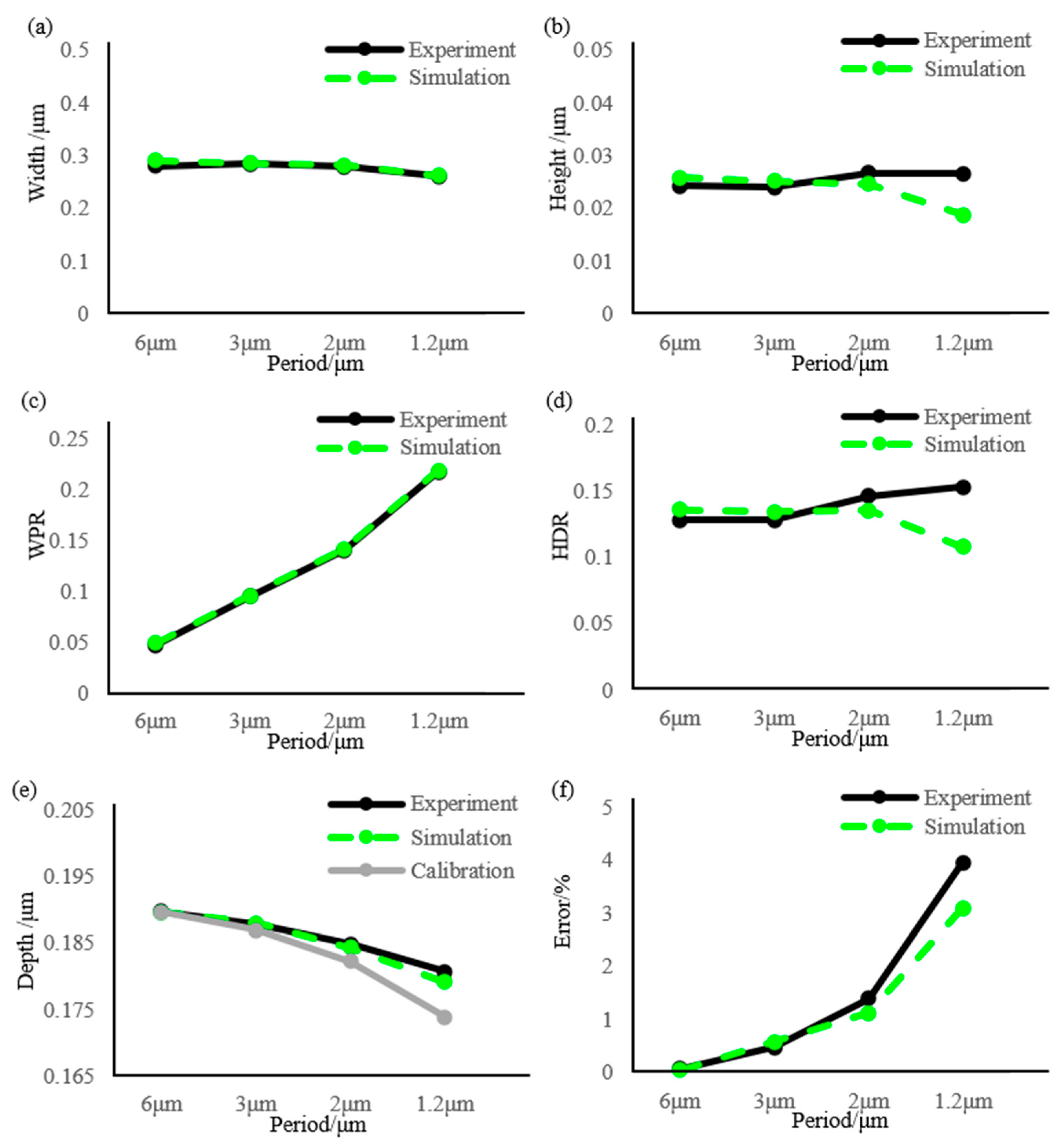
Figure 8a,b show the simulated and experimental batwing width and height for different grating periods, revealing consistent agreement.
Table 3 presents the computed cross-correlation values for
Figure 8a–f. Notably,
Figure 8c,d,f illustrate that the WPR values remain relatively unchanged for gratings with similar depths but different periods. As mentioned previously, when the WPR values are similar and exceed 1/6, there is a positive correlation between the depth measurement errors and HDR values. This relationship arises from the fact that the batwing effect occupies a significant portion of the measured profile for small-period gratings, resulting in considerable depth measurement errors [
5]. As the grating period decreases, the influence of grating diffraction effects on experimental measurements becomes more significant, leading to substantial depth measurement errors for small-period gratings.
4. Conclusions
Accurately quantifying the impact of the batwing effect on grating depth measurements using CSI is crucial for evaluating measurement results. To accomplish this, we determined the height and width of the batwing based on the characteristics that can affect depth calculations from the topography or profile, while utilizing the ‘W/3 rule’. Moreover, we have developed a comprehensive simulation model that integrates the shadow effect, diffraction effect, temporal coherence, and spatial coherence.
Extensive simulations and experimental investigations have revealed significant influences of the NA and the center wavelength on depth measurements. Conversely, the illumination spectrum and shadow effect exert minimal influence on depth measurements. Significantly, we have established that the batwing effect results in substantial depth measurement errors when the WPR values exceed 1/6. Moreover, we have observed a positive correlation between the depth measurement errors and HDR values when the WPR values are similar and exceed 1/6. However, based on our experience, if the grating period exceeds five times the Rayleigh criterion, the ‘W/3 rule’ can accurately determine the grating depths. The proposed model provides a valuable means of evaluating the accuracy of CSI in measuring the depths of rectangular gratings.
In this study, the Fourier model is utilized. When the grating period exceeds twice the Rayleigh criterion and the height is less than the central wavelength, the disparity between the model simulation and experimental results is minimal. However, as the grating period decreases, the inconsistency between the model simulation and experimental results grows. To address the impact of batwing effects on CSI measurement depths for grating periods less than twice the Rayleigh criterion, it is essential to incorporate the effects of grating diffraction and scattering into the model.


