Abstract
In this paper, diffraction of scalar waves by a screen with a circular aperture is explored, considering the incidence of either a collimated beam or a focused wave, a historical review of the development of the theory is presented, and the introduction of the Fresnel approximation is described. For diffraction by a focused wave, the general case is considered for both high numerical aperture and for finite values of the Fresnel number. One aim is to develop a theory based on the use of dimensionless optical coordinates that can help to determined the general behaviour and trends of different system parameters. An important phenomenon, the focal shift effect, is discussed as well. Explicit expressions are provided for focal shift and the peak intensity for different numerical apertures and Fresnel numbers. This is one application where the Rayleigh–Sommerfeld diffraction integrals provide inaccurate results.
1. Introduction
Diffraction by a circular aperture of a uniform plane wave, or focused wave, is an important fundamental topic in optics with numerous applications. Hundreds of papers have been written about this area. Many of these papers have been concerned with applications in acoustics, and a book Scalar Diffraction from a Circular Aperture by Daly and Rao was even published, concentrating especially on the time domain behavior [1]. Another classic source in the optics discipline is the book Waves in Focal Regions by Stamnes, which stresses asymptotic approaches to evaluating diffraction integrals [2].
The aim of the present paper is to reconsider diffraction of monochromatic plane waves, and in particular focused spherical waves, by a circular aperture. We limit our treatment to the scalar case for simplicity, as it will be seen that even the scalar case is quite complicated. Osterberg and Smith calculated the axial intensity for the focused case using the first Rayleigh–Sommerfeld diffraction formula (RSI) and found that under some circumstances the maximum intensity could be situated further from the aperture than the geometrical focus [3]. Li pointed out that because experimentally the maximum should be closer to the aperture, RSI may not always be accurate, as the assumed field in the aperture will not be not correct [4]. He instead calculated the focal shift using a boundary diffraction wave theory. In this paper, we consider different forms of the Fresnel approximation applied to Kirchhoff diffraction theory for diffraction of focused spherical waves. Optical systems with different geometry, dimensions, and wavelength can be compared by introducing normalized optical coordinates.
These results have potential applications in the areas of laser beam systems, micro-optics, diffractive optics, planar optics, teraHertz optics, and microwave lenses.
The obvious further work is to extend the treatment to the vectorial case. The topic of diffraction is very diverse, and any paper cannot cover all areas. Other modern research which could be related to the present study includes diffraction by disks, rather than apertures [5]; diffraction of vortex beams [6,7]; and diffractive optics and meta-lenses [8,9,10].
2. Historical Background
Fresnel diffraction theory is taught in most optics courses and optics text books. Fresnel proposed the principle of half-period zones (∼1818) as a mathematical model for Huygens’ principle of secondary waves (∼1678). The Fresnel number is the number of half-period zones of which an even number tend to cancel by destructive interference. As many papers have discussed Fresnel diffraction, in this section we identify a selection of some key papers in its historical development.
We mention first the work of Young, who proposed a boundary diffraction wave theory (BDW) of diffraction in which the diffracted field can be considered as a summation of a direct beam and a wave scattered from the boundary of an aperture [11].
Airy derived the diffracted intensity for a circular aperture, the Airy disk [12]; his result was in the form of a power series expansion, as this predated the general use of Bessel functions.
Huygens’ principle was placed on a rigorous mathematical basis by Kirchhoff, who applied Green’s theorem over a closed surface to provide the Kirchhoff integral theorem (∼1882), although Helmholtz had previously derived a related result in the frequency rather than the time domain (∼1859). Kirchhoff went on to propose that for diffraction by an aperture in a screen, the field and its normal derivative within an aperture can be assumed equal to their values in the absence of the screen, while the field on the screen and elsewhere on the closed surface of integration can be taken as zero. These are known as the Kirchhoff (or physical optics) boundary conditions. The combination of the Kirchhoff integral theorem and Kirchhoff boundary conditions is called the Kirchhoff diffraction theory. This theory can be applied over a variety of different surfaces, including a planar surface within the aperture (which we call Kp) or over a spherical wavefront (Ks).
In the conventional Fresnel approximation, a square root in an exponent in the diffraction integral is approximated using a power series expansion. Fresnel theory for diffraction by a circular aperture results in integrals that can be evaluated analytically in terms of Lommel functions of two variables, , [13,14]. The functions are used in the illuminated region, as they converge quickly, while the functions are used in the shadow region. The two variables (transverse and axial , respectively) are so-called optical coordinates, dimensionless quantities that allow the resulting intensity to be expressed in a way that is independent of the wavelength and the system geometry and dimensions. This property is quite useful, as even if the field can be computed for specific cases it is difficult to appreciate the overall performance and trends. The same functions can be used to investigate the important cases of diffraction by a circular aperture of a collimated wave or a focused wave in the paraxial approximation. For illumination with a collimated plane wave, the axial optical coordinate u is related to the Fresnel number (the number of half-period zones) , where a is the radius of the circular aperture, z is axial distance, and is the wavelength. The transverse optical coordinate is , where and R is the cylindrical radius, meaning that . Nijboer developed an alternative expansion for the focal field of a lens with circular aperture [15]. Boersma proposed that this expansion can be used for efficient numerical calculation of the Lommel functions [16].
Lord Rayleigh (1891) conducted an analysis of the pinhole camera (camera obscura) [17]. He found that light diffracted by a circular aperture illuminated with collimated light comes to a focus at a distance corresponding to about , which corresponds to the situation where the phase difference between marginal and axial rays is equal to , meaning that there is a single Fresnel zone. Note that an aperture illuminated with collimated light is analogous to a lens with infinite focal length, and the focus is closer to the lens than infinity, meaning that this can be considered as a simple example of focal shift. Rayleigh went on to say that if the distance is increased such that , then the phase difference is reduced to , which reduces the wavefront aberration (defocus) but also reduces the brightness.
Rayleigh (1897) derived the Rayleigh diffraction formulae, in which the integrals are performed over an infinite planar surface [18]. Rayleigh considered an aperture illuminated with a plane wave; the more general case where Kirchhoff-like boundary conditions are applied results in the Rayleigh–Sommerfeld diffraction formulae [19]. There are two Rayleigh–Sommerfeld diffraction formulae, which we call RSI and RSII. Note that the literature does not seem to be consistent in naming the two Rayleigh–Sommerfeld integrals, which seems to result from the fact that Rayleigh considered RSII first, as it is physically relevant for acoustic waves. Our notation (the most common) is that RSI uses a known field on the integration boundary surface and RSII uses a known field derivative. The predicted field from Kp is the mean of RSI and RSII: . The difference between RSI and RSII lies in the resulting obliquity factors. Under many practical conditions, they provide identical results; however, in the far field of a small simple planar source, the field predicted by RSI has a factor , where is the angle of diffraction, equivalent to the planar source behaving as an axial dipole.
Debye (1909) proposed his diffraction theory of focusing, which is basically an angular spectrum theory in which the aperture is assumed to be in the far field relative to the focus [20]. The theory is often further approximated into a paraxial Debye theory [14].
In the acoustics discipline, several papers on the diffraction of convergent beams were published that do not seem to have become well known by the optics community. Williams investigated the acoustic field excited by a concave piezoelectric crystal [21]. He found that the peak in intensity did not coincide with the geometrical focal point, but was displaced towards the crystal. This effect is now known in optics as focal shift. Later papers in acoustics were by Fein, who mentioned that [22]
“Focusing measurements show agreement with A. O. Williams’ prediction that the point of maximum acoustic intensity in the radiation pattern is not necessarily at the centre of curvature of the crystal,”
by O’Neil, who analyzed the system and found that [23]
“The point of greatest intensity is not at the centre of curvature …,”
and by Lucas and Muir [24]. All of these papers found a focal shift towards the aperture, i.e., a negative distance from the geometrical focus.
Andrews studied diffraction of a plane wave by a circular aperture using microwave experiments and Kirchhoff diffraction theory [25]. He found that the positions of the intensity maxima and minima were satisfactorily predicted by the Fresnel zone theory even if the field within the aperture varies in amplitude.
Based on spheroidal wave functions, Bouwkamp developed a rigorous theory of diffraction of an acoustic plane wave by a small circular hole [26]. He then developed the analogous theory for diffraction of electromagnetic waves by a hole in a perfect conductor [27]. Numerical calculation of these results becomes more difficult as the diameter of the hole becomes larger than the wavelength. These results were discussed in more detail in a paper which reprinted his PhD dissertation [28]. As far as I know, the treatment of diffraction of a converging spherical wave has not been studied by a rigorous treatment. Bouwkamp published a review paper on diffraction of both scalar and electromagnetic waves [29].
Linfoot and Wolf investigated the field near the focal region for a circular aperture (as well as for annular apertures) based on the paraxial Debye approximation, and plotted contours of constant intensity in the focal region [30]. The plot was later reproduced in Born and Wolf [14]. The corresponding optical coordinates are and , where is the semi-angular aperture and and z are cylindrical coordinates. Thus, for a contour plot of the intensity in a meridional section, contours of constant are parallel to the z and coordinates, respectively, and the intensity in the focal region is symmetrical about the focal plane, meaning that the intensity maximum is at the focal point [14].
Farnell calculated the field distribution of a microwave lens in the scalar approximation [31]. He found that the axial maximum in intensity was found to occur closer to the aperture than the geometrical focus, and confirmed these results experimentally using microwaves [32].
Richards and Wolf investigated focusing by a high numerical aperture (NA) system in the vectorial nonparaxial Debye (angular spectrum of plane waves) case [33]. However, they used a paraxial axial (defocus) optical coordinate , which is not the most appropriate choice for high NA systems.
Based on the first Rayleigh-Sommerfeld diffraction integral (RSI), Osterberg and Smith [3] derived an exact expression for the amplitude distribution along the optical axis for a focused scalar wave. They found that under certain circumstances the focal shift could be in the positive direction, i.e., further from the aperture than the geometrical focus. For a paraxial system in the Fresnel approximation, the focal shift is found to depend on the value of the Fresnel number.
McCutchen showed that the field in the focal region of a lens can be calculated as a three-dimensional (3D) Fourier transform of a 3D generalization of the lens aperture (related to what is now often called the 3D coherent transfer function, or CTF) [34]. This approach avoids the need for a paraxial approximation.
Kogelnik and Li described the theory, in the paraxial approximation, for propagation of Gaussian laser beams [35]. The focal shift effect is a noticeable property of this theory. In laser optics, the Rayleigh distance ( is called the confocal parameter) is provided by , where is the radius of the beam waist; thus, , where is a Fresnel number associated with the waist of the beam.
Sherman showed the equivalence of the formalism for angular spectrum of plane waves and the RSI diffraction integral [36]. Note that this equivalence holds for the complete RSI diffraction integral, including a factor , and including evanescent waves. Analogous angular spectrum theories also hold for RSII and the Kirchoff diffraction theory with integration over a planar surface (Kp).
Dainty extended the contour plot of intensity for diffraction of a focused wave by a circular aperture for the paraxial and large Fresnel number case to larger values of u [37]. He suggested that intensity zeros occur only in the focal plane and along the optical axis.
Zemanek calculated the diffracted field from a planar circular acoustic transducer, and confirmed Rayleigh’s result that the best focus was when [38]. He started from the Huygens–Fresnel diffraction formula (without an obliquity factor) and calculated the integral exactly, i.e., with no Fresnel approximation. He presented contour plots of intensity, and remarked that
“Two surprising features become evident from examining these figures…. The first feature is that the dB contour has a minimum diameter or spot size of less than one-fourth the transducer diameter.”
This is reminiscent of the reduction in cross-section of a water spout when emanating from a circular orifice.
Heurtley calculated analytic expressions for the axial intensity for diffraction of a focused wave by a circular aperture using RSII and Kp [39], and presented plots showing the focal shift.
Welford showed that a diffractive lens on a spherical surface can be free from spherical aberration [40]. The curvature of the surface modifies the radii of the Fresnel half-period zones.
Papoulis developed a theory of Fresnel diffraction and Fourier optics for an aperture that involved coordinate transformations of the independent variables of the ambiguity function [41]. He derived a simple expression for the variation in width of a diffracted beam in the paraxial approximation in terms of moments of the amplitude of the incident wave.
Carter calculated the field of a scalar spherically-symmetric source numerically, excluding evanescent waves [42]. This is equivalent to the problem of focusing a complete uniform hemispherical converging wave, i.e., . He also presented a plot of the intensity for a semi-angle of convergence of .
Arimoto applied the Fresnel approximation to a lens with circular aperture. He found there was a factor in the axial amplitude, and showed that the point spread function of an optical system of low NA (for a constant focal length) is not symmetrical about the focal plane [43]. He stressed that this effect becomes particularly important for the focusing of laser beams:
“The large f-number optics will become more important as the laser becomes more popular.”
Harvey showed that the breakdown in the Fresnel approximation close to the aperture is equivalent to the introduction of aberrations [44].
Southwell discussed the connections between the Fresnel approximation and the paraxial approximation [45].
The focal shift for optical systems of finite Fresnel number became well known in the traditional optics community only in 1981, when three papers were independently published [46,47,48].
Sheppard and Wilson studied high NA focusing of scalar waves, and introduced a redefined axial (or defocus) optical coordinate , which is a better approximation for nonparaxial systems than the paraxial form [49].
Li and Wolf showed that the optical coordinate of the paraxial Debye theory scales nonlinearly with the axial distance according to the value of the Fresnel number , where f is the focal length and a is the radius of the aperture [47,50]. They found that
The Debye theory is valid only for systems with large Fresnel number values, rather than a small f-number as proposed by Arimoto [43]. For the case of a finite Fresnel number, the paraxial diffraction integral undergoes a coordinate transformation such that the diffracted intensity is not symmetrical about the focal plane. Li and Wolf plotted the intensity in the focal region [50]. Lines of constant u are straight lines perpendicular to the z axis that get further apart with increasing u, while lines of constant v are straight lines that radiate from a point at the centre of the aperture. Born and Wolf’s Principles of Optics was revised (from the 6th corrected edition, in 1986) to provide conditions of validity for the paraxial Debye approximation [51]:
“However if , and , the Debye integral can be expected to give a good approximation to the light distribution in the region of focus.”
Li and Wolf derived an expression for the fractional focal shift for the paraxial case as [47]
Wilson and Sheppard analyzed diffraction of a focused wave by a circular aperture using Fresnel diffraction theory in the paraxial approximation, and showed that there is a paraboloidal phase factor in the focal plane [52]. In addition, they showed that the axial optical coordinate for a point at a distance z from the focus is
only if . Thus, it can be seen that the paraxial Debye form for the axial optical coordinate u makes the assumption that .
Li [53] calculated the focal shift for a nonparaxial scalar system based on the BDW theory. He found that the focal shift effect could be expressed as a function of two parameters, namely, the Fresnel number N and the f-number. Experimental confirmation of the focal shift effect for visible laser light was demonstrated by Li and Platzer [54]. In particular, it was found that the focal shift relative to the geometrical focal point was towards the aperture.
Sheppard described how the focal shift effect for a low NA system could be explained by a compromise between an increase in spatial frequency cut-off for observation points closer to the aperture and blurring caused by defocus [55]. According to this theory, the axial optical coordinate is modified to become , where the effective semi-angular aperture at the observation point is a function of axial position.
Li extended the results of his previous paper on the coordinate transformation resulting from finite Fresnel number in a Fresnel approximation calculation to small Fresnel numbers, including [56].
Sheppard and Matthews proposed the pseudo-paraxial diffraction theory of focusing [57]. According to this theory, the focused field for a system of moderate NA is better approximated by the paraxial approximation if the axial optical coordinate is redefined as [49] such that (the axial component of the phase change along a marginal ray). They also showed that the amplitude of a full uniform spherical focused wave with its maximum intensity normalized to unity is , where r is the spherical radius.
English and George extended the treatment of Osterberg and Smith for the on-axis amplitude for illumination of a circular aperture by a plane wave to provide an analytic expression for the vectorial regime [58].
Steane and Rutt derived an expression for the transverse derivative of the amplitude for illumination of a circular aperture by a plane wave in the Fresnel approximation [59]. They showed that the accuracy of the Fresnel approximation can be improved by redefining the Fresnel number, and thereby the axial optical coordinate.
Bertilone calculated an analytic expression for the focused field at the focus of a uniform hemispherically-focused scalar wave in terms of Lommel functions [60,61].
Kraus proposed calculating the Huygens–Fresnel diffraction integral for diffraction of a diverging spherical wave by a circular aperture by integrating over the wave front rather than the plane of the aperture [62]. He claimed at the time that this approach was more accurate, but later showed that if the full Kirchhoff diffraction integral is used (rather than Huygens–Fresnel) there is in fact no advantage from the point of view of accuracy [63].
Sheppard and Hrynevych [64] provided expressions for the optical coordinates in the nonparaxial finite Fresnel number regime based on a generalization of Fresnel diffraction. In this theory, the optical coordinates are redefined taking into account the critical points in a stationary phase treatment. However, this is not an asymptotic evaluation, and as such is valid even at the focal point. They went on to consider oblique illumination, and derived expressions for the optical coordinates in the meridional plane. The validity of this approach is supported by Young’s BDW theory [11] and the results of Andrews [25]. The accuracy of the generalized Fresnel diffraction theory for diffraction of a plane wave by a circular aperture was investigated in detail by Hrynevych [65]. He found that the results for intensity were accurate to for , as compared with for the conventional Fresnel theory, while for the phase they were accurate to for as compared with for the conventional Fresnel theory.
Andrés et al. studied the off-axis focal shift for non-rotationally symmetric apertures [66].
Hsu and Barakat [67] calculated the focal distribution for a finite Fresnel number system of high NA. They assumed, however, that the distribution could be expressed in terms of Li and Wolf’s optical coordinates, which are not the most appropriate choice for high NA systems.
Wang et al. investigated the far-field behaviour of focused fields for different Fresnel numbers [68,69]. Their numerical results were restricted to the paraxial domain.
Forbes investigated the accuracy of the Fresnel approximation for diffraction of a plane wave by a circular aperture [70].
Sheppard and Török [71] reinterpreted the numerical results of Li [53] using different definitions for the focal length and Fresnel number, which are more appropriate for high NA.
Sheppard and Török considered different power series expansions of the square root in the diffraction integral and derived different optical coordinates corresponding to these expansions [72]. They also considered the vectorial focused case.
Sheppard stressed the requirement for satisfaction of the Debye approximation, i.e., that the axial displacement z must also satisfy in addition to the conditions mentioned by Born and Wolf ( and ) [14,73]. The condition is necessary in order for the paraxial Debye approximation to be valid.
Sheppard and Török calculated the axial field, axial optical coordinate, and focal shift for systems with a high NA and finite Fresnel number based on various different scalar diffraction formulae [74]. For RSI, they confirmed the conclusion of Osterberg and Smith [3], namely, that the focal shift can be in the direction further from the lens than the geometric focus. They considered five different diffraction theories: RSI, RSII, and Kirchhoff (Kp) diffraction integrals performed over the plane of the aperture, a Kirchhoff diffraction integral over the spherical illuminating wavefront (Ks), and an approximate form of Ks valid for small displacements (which we call aKs). Of these, only RSI resulted in positive focal shifts.
Teng et al. showed how the amplitude on the axis and along the shadow edge for diffraction of a plane wave by a circular aperture can be calculated analytically using series of Bessel functions, as these are equivalent to Lommel functions [75].
Li reproduced Osterberg and Smith’s results for RSI; as the occurrence of positive focal shift does not agree with experimental observations, he deduced that RSI is not an accurate diffraction model for this application [4]. Although RSI is rigorous for a scalar approximation, the assumed boundary condition, that is, that the field in the aperture is unperturbed by the presence of the screen, may not be valid. Using BDW theory to correct for the field in the aperture, they were able to obtain negative focal shifts.
Lin et al. used McCutchen’s approach involving 3D Fourier transformation to calculate a focused field of finite Fresnel number in the paraxial approximation [76]. Kou et al. extended this approach to the nonparaxial regime using a 3D RSI model [77].
Glückstad and Madsen described how the predictions of Fraunhofer diffraction by a circular aperture can be extended into the Fresnel regime by renormalizing to the axial amplitude, which can be very simply calculated by the Fresnel diffraction expression [78].
A recent paper by Li considered the complete field, from the aperture to infinity, for diffraction of a focused wave in the paraxial case [79]. He introduced a mapping from the axial coordinate z to a new coordinate (where ) in order to plot the behaviour in the far field. He showed that there are a finite number of intensity zeros between the geometrical focus and infinity.
Several papers have extended the treatment for finite Fresnel number and high NA to the case of oblique illumination [2,80,81,82,83,84,85]. These results have applications in digital deconvolution with objective lenses of finite tube length, although this utility has been reduced by the current adoption of infinite tube length objectives.
It is apparent from this historical review that the traditional optical community was rather slow to appreciate several features of diffraction that were well known in other disciplines, including laser beam optics, microwave optics, and acoustics. It is interesting to recall the rebirth of optics in the 1960s, which resulted from the introduction of optics and photonics into the electrical engineering curriculum through developments in lasers and quantum electronics, electromagnetic theory and microwaves, and information and Fourier optics.
3. The Fresnel Approximation
3.1. The Two Traditional Forms for the Fresnel Approximation (FrA1 and FrA2)
We first review the case of diffraction of a uniform plane wave by a circular aperture in order to introduce the Fresnel approximation. For illumination of a circular aperture by a uniform plane wave, the Huygens–Fresnel (HF) diffraction integral (neglecting an obliquity factor) becomes
where r is the distance from a point in the aperture to the observation point, with
Here, represents a spherical wave emanating from a point in the aperture and the factor comes from the fact that the source is driven in resonance, meaning that the far field is out of phase with the forcing.
Although it sometimes might not be appreciated, there are two forms of the Fresnel approximation [44,82]. In the first (FrA1), we replace r in the exponent by expanding the square root by a binomial expansion:
where are cylindrical radii in the aperture and observation planes, respectively. In the second form (FrA2), we divide by the distance from the centre of the aperture to the observation point:
The difference between these approximations is that if is large, cannot be assumed to be small, as in Equation (6).
In the denominator, r is replaced by the first term of the expansion Equations (6) and (7). Then, the diffracted amplitude (for FrA1) is
or
for FrA2, where is a Bessel function of the first kind of order n. For FrA1, the exponential before the integral represents a paraboloidal wave, while for FrA2 it represents a spherical wave.
Setting , we can introduce optical coordinates (FrA1) or (FrA2) to obtain
where
A third optical coordinate w has now been introduced:
where can be expressed in terms of Lommel functions of two variables . The factor of 2 in Equation (11) ensures that for .
Contours of u and v are plotted against and in Figure 1 and Figure 2 for FrA1 and FrA2, respectively, where the variable , the shadow edge corresponds to , and small (small u) corresponds to the far field. Lines of constant v are straight lines in both cases. They are very similar for small values of v but become more different as v increases. Lines of constant u are straight lines for FrA1 and circles for FrA2. They agree quite well for small and larger than about three.
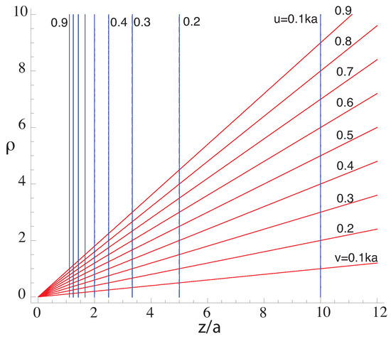
Figure 1.
Contours of u (blue) and v (red) for FrA1 for diffraction of a plane wave by a circular aperture.
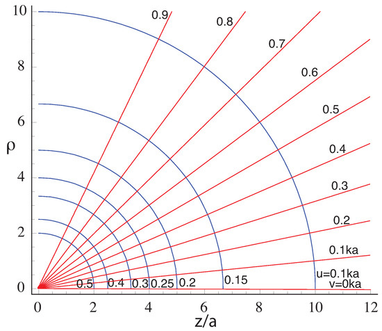
Figure 2.
Contours of u (blue) and v (red) for FrA2 for diffraction of a plane wave by a circular aperture.
The advantage of FrA1 is that it allows the field to be propagated from a plane to a plane. However, FrA2 is more accurate than FrA1 in the far field for large values of , when the field strength can be significant for small apertures. It should be appreciated that although the intensity can be expressed in a way that is independent of wavelength and geometry, the phase cannot because of the factor .
3.2. The Generalized Fresnel Approximation (gFrA)
The Fresnel approximation uses a parabolic approximation of r evaluated by a power series expansion that becomes worse as increases relative to z or . This is unfortunate, as we know from the stationary phase method that the edge of the aperture makes a significant contribution to the integral. Thus, alternative ways of matching can be expected to provide an improved result [59]. In the generalized Fresnel approximation (gFrA), we still use a parabolic approximation, but choose to match up at the critical points of r in the stationary phase evaluation of the diffraction integral [64]. However, we do not actually use a stationary phase expansion, and only use it to define the optical coordinates, meaning that the approach is valid even in the focal region. Here, we have
In the illuminated region, there are three critical points, two of the second kind and one of the first kind, which provide three simultaneous equations for . We introduce , respectively the maximum and minimum distances from the observation point to the aperture edge, as follows:
Then, the two critical points of the second kind provide the two equations
where the + and − signs refer to and , respectively. Subtracting the two parts of Equation (15), we obtain the transverse optical coordinate
such that surfaces of constant v are hyperboloids of one sheet, with the foci located on the aperture edge. Contours of constant v are shown in Figure 3. If and are large enough, then lines of constant v tend asymptotically to straight lines, the slopes of which agree better with FrA2 than FrA1.
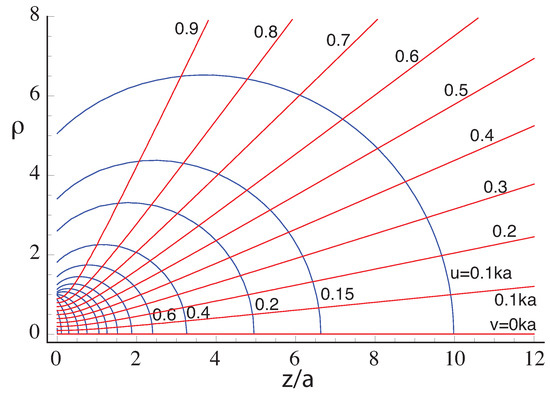
Figure 3.
Contours of u (blue) and v (red) for the generalized Fresnel approximation for diffraction of a plane wave by a circular aperture.
Additionally, adding the two parts of Equation (15), we have
The third simultaneous equation is provided by the critical point of the first kind:
Eliminating w, we have
which are positive, and which we can set equal to , , respectively. results in slow intensity variations, while results in fine structure. We introduce the variables , defined as [64]
resulting in . It is difficult to appreciate the behaviour of for large z from Equation (20); thus, we rewrite them here as
where we have used .
Then, the other two optical coordinates are
Contours of constant u are shown in Figure 3. These are plotted over a larger domain than our previous plot [64], and are more accurate as a result of improvements in the contour plotting routines. Lines of constant u become close to circles for small values of u. For small , they match FrA2 quite well for values of greater than about four. For larger values of u (greater than about ), lines of constant u become more elongated and the shape of the lines for FrA1 agree better than those for FrA2, although neither of the standard Fresnel approximations provides the correct relationship between u and . Contours of constant w are shown in Figure 4. For large w these are approximately circular, becoming more elongated for smaller values of w. For large , it can be seen from Equation (17) that as u becomes small, the equation for constant values of w provide a family of ellipses with the centre at the origin, tending towards spheres for .
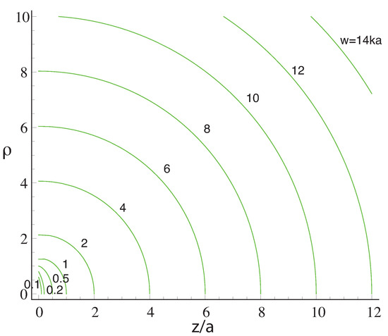
Figure 4.
Contours of for the generalized Fresnel approximation for diffraction of a plane wave by a circular aperture.
Along the axis, and ; thus, and , and we have
Values of , where n is a positive integer, determine the positions of the intensity zeros along the axis. The axial intensity zero furthest from the aperture occurs at
Thus, the number of axial intensity zeros is , indicating the axial behaviour depends on the value of the dimensionless parameter . The axial field agrees well with direct evaluation of the diffraction integral, but only agrees with FrA1 or FrA2 if .
Along the shadow edge, , , , and .
In the plane of the aperture, , , and ; thus, , and within the aperture, and .
For small , we have the following for :
If is larger than about 5 [64], then we have
The radius of curvature of contours of constant u at tends to for large z, i.e., the centre of curvature is at , as can be deduced from Figure 3.
For , we obtain
which indicates agreement with FrA1.
The generalized coordinates work well for the illuminated region. In the shadow region, there are two critical points of the second kind, corresponding to the rim of the aperture. Then, the transverse optical coordinate v is
which is consistent with the previous results (as in Equation (16)). For , if we also have , then
which agrees with FrA2. If, in addition, , then this also agrees with FrA1.
The amplitude and phase of the diffraction pattern can be calculated from Equation (4) using the values of and to provide gFrA-HF. These same values can alternatively be used together with RSI, RSII, or Kp diffraction integrals. The integral should be pre-multiplied by a factor for gFrA-RSI, a factor for gFrA-RSII, and a factor for gFrA-Kp, where is the angle subtended at the axis by the line from the centre of the aperture to the point of observation. For a distant observation point, and can be neglected; however, there will still be distinct angular differences between RSI and Kp relative to the Huygens–Fresnel result. In fact, as is well known in antenna theory, RSI acts as an axial dipole rather than as a simple source. Closer to the aperture, gFrA-RSI reproduces the exact RSI results better than the gFrA-HF predictions [64].
4. The Focused Case
4.1. Focal Length and Fresnel Number
We now consider the case of diffraction of a convergent wave by a circular aperture, considering a spherical wave convergent on an opaque screen with a circular aperture of radius a (Figure 5). We stress that this is different from the case of a microscope objective used to focus light to a small spot, where the aperture is situated in the front focal plane of the lens and Fresnel number effects are not present. We define the focal length as the radius of curvature f of the wave front at the aperture. This is different from the usual convention in paraxial optics, which is the distance d of the focus from the plane of the aperture. If the focal length of the lens is long, then these tend to the same value; however, in the limiting case of a hemisphere of focused wavefront, , where is the semi-angular aperture of the focusing system. We choose to specify either or the NA rather than the f-number , as the f-number becomes zero for the hemispherical case in which .
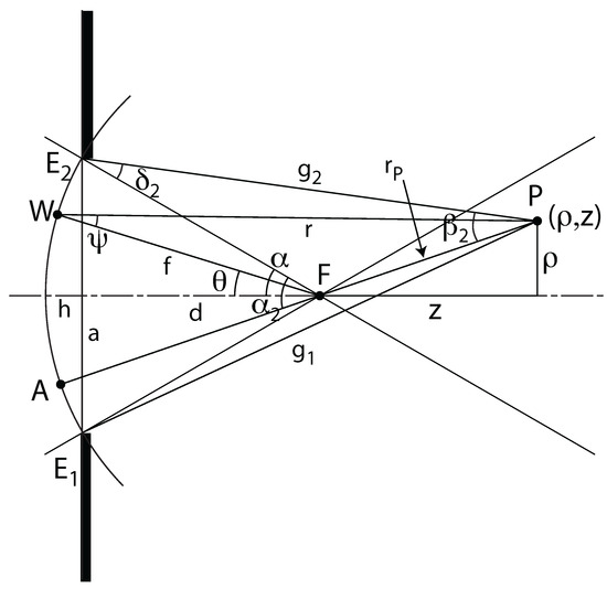
Figure 5.
Schematic diagram of a spherical wave diffracted by a circular aperture of radius a in an opaque screen at distance d from the geometrical focal point F, with sagitta ; the angle is the semi-angular aperture, and is the angle subtended at the optical axis by a ray from a general point W on the wavefront to F. The points on the aperture edge correspond to the maximum and minimum distances from the observation point P, with cylindrical coordinates relative to F and distant from F and r from W. The triangle has an exterior angle and interior angles and . The angle rays between rays from point W to F and P are .
We define the Fresnel number as the number of half-wavelengths in the difference between the distances of the geometrical focus from the edge and centre of the aperture; thus, . This definition is different from the definitions used by Li and by Hsu and Barakat (which are also different from each other) [53,67]. Note that is related to the surface area of the cap of the spherical wavefront by , which determines the amplitude at the focal spot. The significance of the Fresnel number of half-period zones is that the field for an even number of zones tends to cancel by destructive interference to give a zero, while for an odd number of zones there tends to be close to a secondary maximum in intensity. This definition of Fresnel number is consistent with Welford’s proposal for generating diffractive lenses on spherical surfaces to eliminate spherical aberrations [40]. For a low NA, is small, meaning that and ; however, this latter expression does not accurately provide the number of Fresnel zones for higher NA. A consequence is that the radii of the regions in a zone plate, conventionally , need to be modified at higher NAs [40]. Indeed, for the hemispherical case, , while the paraxial form becomes infinite. Even for the complete spherical case, is still defined, providing ; however, N is only defined for . Moreover, as must be non-zero, implies that .
Li argued that RSI is not valid for the case of high NA focusing by a system of finite Fresnel number [4], as the calculated focal shift can be positive, as calculated by Osterberg and Smith [3], whereas in practice negative values are always observed. In addition, negative focal shift would be intuitively expected by analogy with Gaussian beams, where the waist of a focused wavefront occurs before its centre of curvature. The problem with RSI is that, although it is exact, the assumed amplitude within the aperture (equal to the amplitude if the screen with aperture were absent) is not correct. For this reason we agree with Li, and choose not to use RSI.
The amplitude in the focal region of a lens can be alternatively calculated using the Kirchhoff diffraction integral, which is known to be exact when performed over an arbitrary closed surface. We choose to integrate over the spherical wave front (Figure 1), an approach we call Ks (for Kirchhoff, spherical). Note that while this has similarities with the approach of Kraus, it is different in that we apply integration over the wave front for a converging wave rather than for a diverging one [62]. We assume that the field on this surface is equal to the incident spherically-convergent wave (Kirchhoff boundary condition), and the field on the remainder of the closed surface is taken as zero. We argue that this assumption is more accurate than either of the RSI and RSII Rayleigh–Sommerfeld approaches, where the integral is performed over a planar surface (or, in the Kirchhoff approximation, performed by integrating over a plane, which we call Kp) because the presented method incorporates effects of diffraction during the propagation of the wave before reaching the aperture plane. The obliquity factor for this geometry is close to unity, and as such can be neglected for observation points not too distant from the geometrical focus, even though the convergence angle is appreciable. This is very different from the geometry for a planar integration surface or diverging wave as studied by Kraus [62,63]. We continue by neglecting a term of order . Then, the amplitude at a point P with cylindrical coordinates relative to the geometrical focus is
where
4.2. Behaviour along the Optical Axis
We first consider the amplitude U at a point on the axis at a distance z from the geometrical focus when
and
Li and Wolf presented an evaluation based on series expansion of the square root, resulting in a form of the Fresnel approximation [50,72]. However, rather than approximating the square root, which can introduce inaccuracies, we choose to evaluate the integral in Equation (32) directly for an observation point on the optical axis. This approach was described previously in [74]. Thus, changing the variable of integration from to r using from Equation (33), we have
where the distance g of P from the centre and edge of the aperture is
Geometrically, Equation (34) can be recognized as comprising two components, representing the sum of two waves from the centre and edge of the aperture, respectively (as in Young’s BDW approach) added in antiphase. The axial amplitude is then provided by
Therefore, to describe the axial amplitude, we introduce the axial (defocus) optical coordinate u, defined in terms of the argument of the sine function in Equation (36) as follows:
This definition for the axial optical coordinate has previously been discussed elsewhere [64,71,74].
Then, for the axial amplitude we have
where the phase variation (unwrapped) along the axis relative to the geometrical focal point is
This expression for the axial amplitude is a generalization of the paraxial Debye expression ([14], p. 441) but is valid for both large angles of convergence and finite values of the Fresnel number. Thus, the axial intensity is
From Equation (37), it is difficult to see the behaviour of u when z is small; we can rewrite the equation as
Now, , with a mapping
In a similar way, is provided by
We can obtain an equation between u and z by eliminating g from Equations (35) and (37):
which can be solved for as a function of u:
We now introduce the Fresnel number , where . For in terms of , we have
which is plotted in Figure 6a for different values of . In Equation (46), we have introduced a dimensionless parameter . All the curves exhibit the same slope for small . For small (or for large , and consequently large ), we have , agreeing with the result of the pseudo-paraxial treatment [57], while for u reduces to the form of Li and Wolf for the finite Fresnel number case in the paraxial approximation [50]. For large values of , , meaning that there is a finite number of zeros in intensity beyond the geometrical focus. In the centre of the aperture , unlike in the paraxial case, is also finite. Interestingly, for , corresponding to extreme case of a complete spherically focused wave, and , agreeing with the correct values for a spherical standing wave [57]. This gives us confidence that the diffraction integral is providing meaningful results.
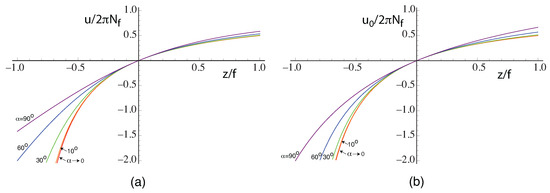
Figure 6.
The behaviour of (a) (from Ks) and (b) (from aKs), with for different semi-angular apertures. Lines are coloured red for small , orange for , green for , blue for , and purple for . For small , the behaviour of and agrees with that of Li and Wolf [50]. Along the optical axis, , with Z as in Equation (42) and D as in Equation (46).
We now have the following for as a function of and :
which was plotted in [74].
We have expressed u in terms of , and z, with the first three parameters characterizing the optical system. There are many alternative ways to specify the geometry. The triangle has sides in general (and similarly for triangle ); for the special case when P is on the axis, it has sides . The angles of the triangle are , where is the exterior angle. For P on the axis, . On the optical axis [74],
Using the sine rule, we have
which, if are small, gives us
which is the same as derived for the paraxial case [55]. Further, if we defines a Fresnel number for the observation point, then , meaning that . Then,
and
The intensity at the geometrical focal point is
Then, the axial intensity is
or in terms of u and ,
For large N, Equation (55) reduces to the standard form for the paraxial Debye approximation as provided by Born and Wolf [14], except that the optical coordinate u is provided by the more correct high NA form [57]. The focal shift effect is caused by the factor in the braces in Equation (55). It can be seen that this factor becomes weaker as NA increases, becoming a constant for a complete spherical wave (i.e., corresponding to no focal shift).
4.3. Focal Shift
The optical coordinate u provided by Equations (37) or (46) is of a more complicated form than that of Li and Wolf [50]. However, if we apply the condition that , which we call aKs (approximate Kirchhoff spherical), we have and can obtain approximate expressions for u from Equation (41):
Note that this equation cannot be derived accurately from Equation (37) in the same way, as is the small difference between two large quantities; thus, we must be careful when using the approximation . A better approximation is . The first equality of Equation (56) reduces to provide the usual high NA expression if is negligible [57], while the second form reduces to the finite Fresnel number expression of Li and Wolf when is small [50]. Thus, Equation (56) can be regarded as providing more accurate expressions for the optical coordinate in the regime with finite Fresnel number and high NA that are valid for small distances from the geometrical focus. We can further introduce , approximate values of , valid near the geometrical focal point. Then, we have , . It should be noted that Hsu and Barakat [67] assumed the paraxial form for the optical coordinates in their high-aperture vectorial treatment based on the Stratton–Chu formula, which is not justifiable for high NAs. The behaviour of with is shown in Figure 6b. It can be seen that the range of values of for which is a good approximation for u increases as NA decreases.
If is small, then for the analogous approximate expression for we have
which reduces to the high NA axial phase variation for [57].
The approximate form for u is valid for small focal shifts, meaning that the principal maximum in intensity is located at
Then, the fractional focal shift is provided by
and the increase in intensity relative to that at the geometrical focus by
Equations (58)–(60) are generalizations of those of Li and Wolf for low NAs [47,50]. Further, Equation (59) for the fractional focal shift is much simpler than the empirical formula provided by Li for the nonparaxial case [53]. As we have seen that implies that , in this case Equation (59) provides , meaning that the axial intensity decays monotonically from the aperture plane [79]. For non-zero , as the value of cannot be less than from geometrical arguments, there is a minimum Fresnel number predicted by Equation (59) for any given value of . For example, the minimum Fresnel number is for , corresponding to a value of and .
Figure 7 compares the fractional focal shift predicted from the Ks expression for intensity in Equation (40) using Equation (46) and by the analytic expression in Equation (59) provided by aKs. The behaviour calculated from Equation (40) and aKs show good agreement. The fractional focal shift is negative, showing that the diffraction focus is shifted towards the aperture for all NAs, in contrast to Osterberg and Smith’s results using RSI for high NA (, ) [3] (and confirmed by [4,74]). The absolute value of the fractional focal shift increases as the Fresnel number decreases. For Ks, the absolute value of the fractional focal shift decreases with NA for Fresnel numbers greater than about 0.62 and increases for smaller values of Fresnel number. The behaviour predicted by the aKs analytic expression in Equation (40) is qualitatively similar, but the effect of NA is smaller, with the cross-over for no variation in focal shift with aperture occurring at a Fresnel number of for low NAs. For high NA, as decreases the size of the aperture also decreases, and eventually the diffraction calculations become invalid. We indicate where in Figure 7 the value of () by coloured circles.
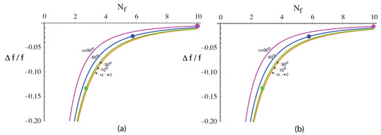
Figure 7.
The fractional focal shift as a function of the Fresnel number N for different NAs: (a) for the Ks model (Equations (46) and (55)) and (b) from the analytic aKs expression in Equation (59). Lines are coloured red for small , orange for , green for , blue for , and purple for . For small , the behaviour agrees with that of Li and Wolf [50]. The curves for small and are very close to each other. The small circles indicate where : for small , the Kirchhoff boundary conditions tend to break down.
4.4. Off-Axis Behaviour
We now wish to generalize to off-axis observation points. Although Equation (30) can be evaluated exactly for points on the axis, unfortunately this cannot be done in general; thus, we wish to approximate it. In [57,64], we approximated it to the Fresnel diffraction integral, which has analytic solutions in terms of Lommel functions. We called this the pseudo-paraxial approximation. However, as the NA increases, the field calculated by the Fresnel diffraction integral departs from that predicted by the Debye integral (angular spectrum) method. Therefore, here we choose to approximate to the scaled Debye–Wolf (sDW) approximation, as the (unscaled) Debye–Wolf (DW) form provides better agreement for higher NAs and large Fresnel numbers than the pseudo-paraxial approximation [57,71]:
where the optical coordinates are scaled as follows:
by the mappings to approximate r in Equation (31) by
Note the opposite sign of u in Equation (61) as compared with the collimated case in Equation (11). This is consistent with the fact that for the collimated case u was defined as positive and increasing towards the aperture, as in Figure 3. The diffraction integral no longer has variables in the Bessel and complex exponential functions of the simple forms , as they are in the paraxial Debye or the Fresnel approximations. Along the axis, , it reduces to the Ks of Equation (38).
For the (unscaled) DW equation, then, , , and , and it is valid for high NAs in the scalar approximation, though only for large values of the Fresnel number. Thus, the normalized axial intensity is regardless of the value of , even up to ; however, the transverse intensity in the focal plane varies from an Airy disk for small to for both and .
For smallish such that , Equation (61) reduces to the pseudo-paraxial form, with analytic solutions provided in terms of Lommel functions. For large Fresnel numbers, , , and , meaning that , and for a marginal ray subtending an angle of we have
by which it can be seen that axial scaling is more correct than the paraxial treatment in Born and Wolf, which gives [14].
For very small , sDW reduces to the fully paraxial form when . This is the case for the mapping , discussed by Li [79].
4.5. The Debye–Wolf (DW) Integral
Bertilone provides an analytic expression for the focal field for the (unscaled) DW case for [60,61]. Then,
where is a Lommel function of two variables and is taken as ±ve for . This expression is equivalent to the (unscaled) Debye–Wolf integral. Useful properties of the Lommel function are that and . A numerically calculated contour plot of the intensity was presented earlier by Carter, who provided a plot for as well [42]. The intensity in the focal region, calculated directly from Bertilone’s expression, is shown as contours in Figure 8d [86], where it is compared with the paraxial Debye case (i.e., for small ) in (a) and with the nonparaxial DW plots for and in (b) and (c). For , and ; thus, . While the overall features of the contour plots are all similar, there are differences in their sidelobe structures. Carter’s plot for shows that the overall pattern of the maxima and minima in intensity exhibit alignment of features along lines of constant v and along circles with the centre at the focus [42].
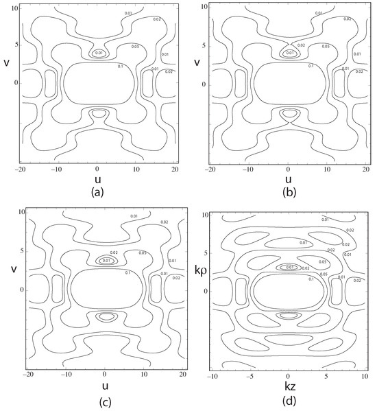
Figure 8.
Contours of constant intensity in the focal region of a focused scalar wave diffracted by a circular aperture in the Debye approximation: (a) for a small semi-angular aperture , (b) for the nonparaxial Debye case for , (c) for the nonparaxial Debye case for , and (d) for , computed from the analytic expression in Equation (65). The intensity at the focal point is normalized to unity. An analytic plot for was first shown in [86].
4.6. The Scaled Debye–Wolf (sDW) Case
In the sDW case, for the illuminated region we match r and its approximation at the three critical points in the stationary phase expansion of the integral; note, however, that we do not use an asymptotic evaluation of the integral. For observation points close to the geometrical focus, even though the stationary phase asymptotic method cannot be used, the expansion is still valid. The two critical points of the second kind give
where are the maximum and minimum distances of the observation point from the aperture edge
Adding and subtracting, we have
where . The second of these equations defines R and v valid for the whole of the focal region, whether illuminated or shadow:
Surfaces of constant R are hyperboloids of one sheet:
Close to the axis, such that , we have , . If is small, then the surfaces of constant R tend to cones with the vertex at the centre of the aperture and , agreeing with Li and Wolf [50].
The first line of Equation (68) contains both W and Z, and as such cannot be solved independently for these. We note that on the axis it reduces to Equation (39), meaning that and . However, for the illuminated region there is a third critical point corresponding to matching up the values at the maximum or minimum of the two sides of Equation (63), resulting in an additional equation. For the left-hand side, this corresponds to a direct undiffracted ray passing through the geometrical focal point along the line in Figure 5. For the right-hand side, we find the maximum or minimum of the right-hand side of Equation (63). Therefore, the third equation is
Eliminating W using the first line of Equation (68), we have
where we have introduced the variable m, a function of the observation point, which is zero at the geometrical focal point. We take for and for . Equation (72) can then be written as a quadratic equation in Z:
and solved for Z in terms of m using Equation (69):
where we take the positive square root for (inside the shadow edge) or (outside the shadow edge) and the negative root for (outside) or (inside). On the shadow edge, .
The corresponding quadratic equation in the axial optical coordinate u is
and its solution for u is
Along the axis, and . Then, and , as in Equation (37) for the Ks theory. Simply, or , where we take the positive/negative roots in Equations (74) and (76) for positive/negative z, respectively.
In addition, for W we have
Contour plots for and are shown in Figure 9 for different values of , while contours of are shown in Figure 10. The plots cover the domain within a sphere of radius f. For and , contours for constant and are shown in green and blue for and , respectively. In particular, we note that for higher NA the sDW version of Ks can predict the field strength before (i.e., to the left of) the aperture plane, whereas RSI, RSII, and Kp cannot.
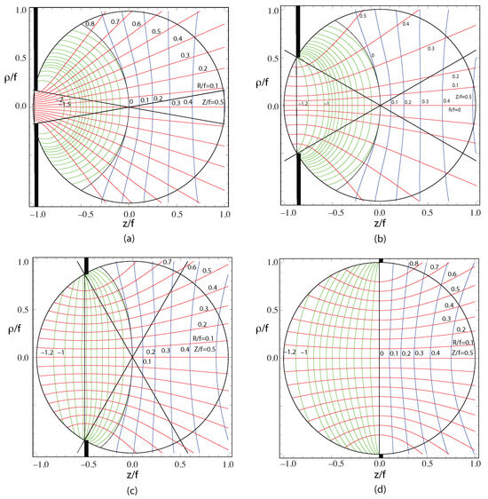
Figure 9.
Contours of (in red) and (in green for and blue for ) for the scaled Debye–Wolf theory for diffraction of a spherical wave by a circular aperture: (a) , (b) , (c) , (d) . The black contour is for . The shadow edge is also indicated in black.
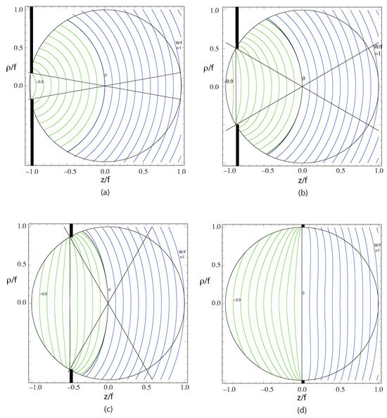
Figure 10.
Contours of (in green for and blue for ) for the scaled Debye–Wolf theory for diffraction of a spherical wave by a circular aperture: (a) , (b) , (c) , (d) . The black contour is for .
Although the third critical point is only present for the illuminated region, we can consider extrapolation into the shadow region as a type of analytic continuation. The slope of the contours for is continuous at the shadow edge. For or , the two contours do not match up completely in each case, but agree well for . This value of corresponds to a larger value of v as increases or decreases. A magnified contour plot of a smaller region is shown in Figure 11. On this scale, the two contours for are almost indistinguishable; only one, , is shown in the plot. However, even for the contours of constant are noticeably curved, unlike in the paraxial treatment of Li and Wolf [50].
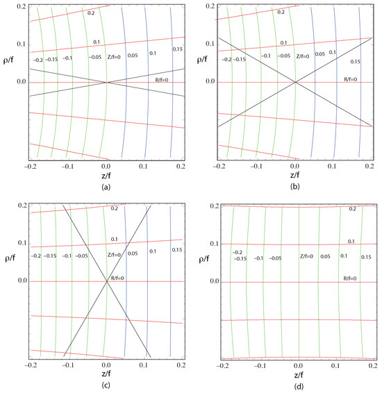
Figure 11.
A magnified view of the contours of (in red) and (in green for and blue for ) for the scaled Debye–Wolf theory for diffraction of a spherical wave by a circular aperture: (a) , (b) , (c) , (d) . The shadow edge is indicated in black. The contours for provided by the two alternative expressions in Equation (74) are almost identical at this scale.
As we have mentioned, the Debye approximation is only valid for regions near the focus [73]. Even for small values of , e.g., , the Debye approximation breaks down for distances from the focal point that are a substantial fraction of f, although of course for large f the intensity is very small in this case. For small , the surfaces for and are approximately spherical, with a radius of 1, agreeing with [52]. The radii of curvature increase with , becoming planar for . In fact, the radius of curvature of Z or W for small is approximately equal to . For small , the contours become approximately flat for , which reduces to the aperture plane for .
The values of and along the shadow edge are shown in Figure 12, where . The behaviour of Z is qualitatively similar to the variation along the axis, as shown in Figure 6.
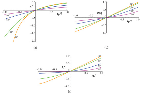
Figure 12.
The variations in (a) , (b) and (c) along the shadow edge. Here, . Lines are coloured orange for , green for , blue for , and purple for .
In the far field, when and , we have
which can be written as a quadratic equation in Z
and solved for Z in terms of m:
where g is defined in Equation (35). In a similar way, the quadratic equation in the axial optical coordinate u is
and its solution for u is
For m, in terms of the spatial coordinates, for and we have
meaning that for Z we have
This expression for Z predicts the behaviour of Z near the optical axis in the far field. We find that the curvature of the contours of constant Z reduce as z increases, then changes sign, reaches a maximum value, and decays as . The position of the sign change agrees well with Figure 9 for or . For , it does not agree, probably because is not sufficiently large for the approximations to be valid.
While the approach used thus far fares well for the illuminated region, the definitions of Z and W become more inaccurate as we move into the shadow region. This is because there are only two critical points in the shadow region. We have defined , and can see from Equation (68) that because constant A corresponds to constant , the surfaces of constant A are oblate spheroids (surfaces of rotation of ellipses about their minor axes) with equations
The corresponding contours of are shown in Figure 13. For small , ; if , then . On the optical axis, from Equations (37), (68), and (62) we have
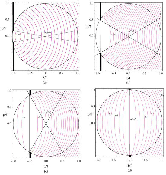
Figure 13.
Contours of for the scaled Debye–Wolf theory for diffraction of a spherical wave by a circular aperture: (a) , (b) , (c) , (d) .
The value of along the shadow edge is shown in Figure 12c.
If , then
The contour for is indicated in Figure 9 and Figure 10. In all cases, this contour lies between the corresponding green and blue contours for both and . Z is small when ; therefore, we propose taking as an approximation that for points in the region between the two alternative contours for , meaning that . In this region, the intensity is very weak anyway, and small values of u result in only a small effect on the intensity. For the conventional Airy disk, the intensity for falls off quickly, as . Interestingly, we find that when , the two solutions for m are equal and opposite in sign; thus, their mean is zero.
For this choice of values, Figure 14 shows the variation in , , and along three lines of constant z () and for four values of equal to , as indicated by colour. For , there is a nonlinear variation in R as a function of (except for , when it is linear) and . The nonlinearity decreases as increases. For , and exhibit break points at the shadow edge, marked by small circles; for , the behaviour is more complicated for and . There are up to three break points, located at the shadow edge and the two points where . Between these, we assign and .
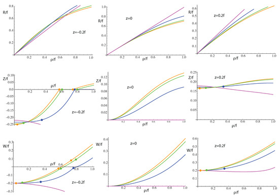
Figure 14.
Plots of (top row), (middle row), and (bottom row) along lines of constant ((left column) , (middle column) , and (right column) ), shown for different values of (indicated by colour, orange , green , blue , and purple ) Break points are indicated by small circles.
This choice of and in the shadow region is only one possible strategy. Another alternative is to take contours of both and in the shadow region to be the same shape as contours for , with the magnitude chosen such that the contours are continuous with those in the illuminated region at the shadow edge. We call this the corrected scaled Debye–Wolf theory (csDW). Figure 15 shows contours of constant and for and . Note that there are now no gaps in the coverage, unlike the previous stategy (sDW), which had a problem with the region around . csDW works well for negative , as the contours are smooth through the shadow edge.
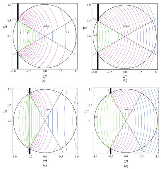
Figure 15.
Plots showing contours of constant (left column: a and c) and (right column: b and d) for (top row: a and b) and (bottom row: c and d) for the csDW theory. Colours: illuminated region, blue , green ; shadow region, purple.
However, for positive the contours of constant have a different shape, meaning that there is a discontinuity of the slope at the shadow edge. Preliminary numerical calculations have shown that the proposed choice of sDW results in better predictions than csDW near the shadow edge for positive z.
In fact, the shape of the contours in the illuminated region for is very similar to that of the contours of , and could be approximated by contours in scaled to match on the optical axis. We call this the approximate sDW theory (asDW). Setting , the z coordinate of the contour on the optical axis is , where the negative sign is taken if . Then, we have
Contours of constant and for and are shown in Figure 16. For , the contours agree well with those for sDW and csDW. For , however, the contours for in particular, although agreeing on the optical axis, exhibit curvatures of opposite sign.
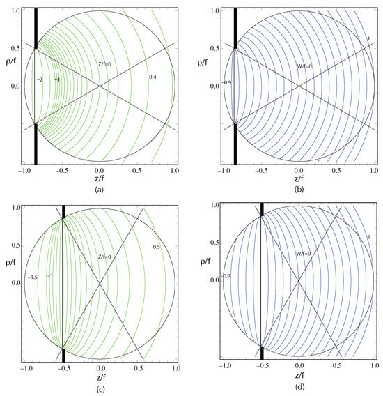
Figure 16.
Plots showing contours of constant (in green) (left column: a and c) and (in blue) (right column: b and d) for (top row: a and b) and (bottom row: c and d) for the asDW theory.
The case for is interesting. As there is no shadow region, the three critical points are valid everywhere, and Bertilone’s analytical solution for the field in the DW case is available. The equations for the optical coordinates also simplify, meaning that and .
4.7. The Pseudo-Paraxial Approximation
In this paper, we have considered the scaled Debye–Wolf approach for approximating the focused field in the finite Fresnel number case as a scaled high-NA field. In a previous paper [64], we studied the pseudo-paraxial theory for a finite Fresnel number, which is not as accurate at high NAs but has the advantage that the analytical Lommel solution is available. This pseudo-paraxial theory is based on the generalized Fresnel approximation, i.e., a quadratic fit of the DW theory is made, matching up at the critical points. It is interesting to compare these two solutions, namely, the sDW and the pseudo-paraxial approximation to Ks. In the pseudo-paraxial approximation, the in Equation (63) is matched to the parabola , where s is a radial variable normalized to unity at the aperture edge . The critical points corresponding to the aperture edge are the same as for sDW, as in Equation (66); thus, the values of are the same as those in Equation (68). The third critical point satisfies the condition
thus, eliminating w,
In this way, we obtain quadratic equations for u or Z:
and solve for u or Z in terms of m:
which reduce to the corresponding Equations (74) and (76) for either small or on the axis. The intensity along the axis is identical to that in the sDW case, and the intensity along the shadow edge is similar for or . However, plots of and (Figure 17) show that the behaviour is quite different from the sDW case, even for . Contours of constant small value of have an opposite sign of the curvature than the sDW case, which means that, although they are the same as sDW close to the axis where the contours are flat, there is actually only a single point, at the geometrical focus, where and . Unlike sDW, there is a region between the two contours for corresponding to different signs of the square roots where the two solutions provide different values for . These factors suggest that the pseudo-paraxial treatment is useful only in the illuminated region or close to it. The contours are similar, though more detailed, when compared to those shown in our previous paper (which were only shown for off-axis illumination) [64]. In our earlier paper, the expressions for were provided in terms of , as in Equation (20) of this paper, whereas in the notation used in the present paper this is and .
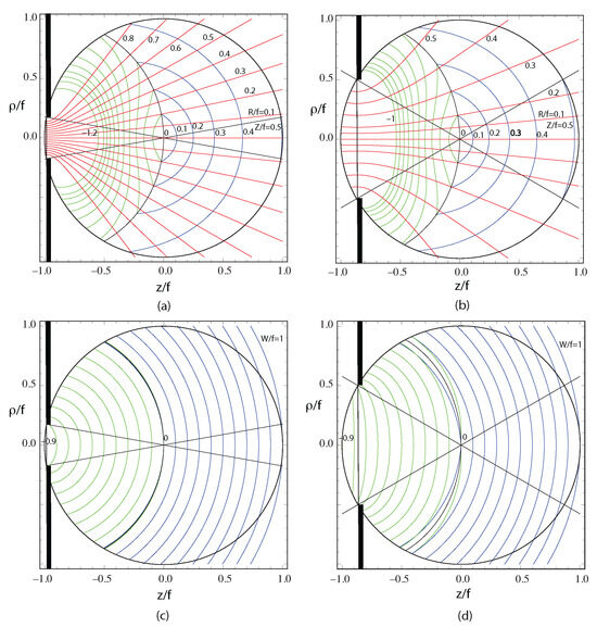
Figure 17.
Contours of (in red), and (in green for and blue for ) for the pseudo-paraxial theory for diffraction of a spherical wave by a circular aperture: (a) and , , (b) and , , (c) , , (d) , . The black contours in (c,d) are for .
In the far field, , near to the axis ,
and
Although the curvature of the contours of Z for positive z in Figure 17 always has the same sign, we actually find that the curvature changes sign at about (reducing as increases).
4.8. The Kirchhoff Diffraction Integral Performed over the Plane of the Aperture (Kp)
For Ks in Equation (34), we found that the amplitude along the optical axis is provided by the destructive summation of equal contributions from a direct wave and a BDW, agreeing with the concepts of Young’s BDW theory. Exact solutions for the amplitude along the optical axis predicted by RSI, RSII, and Kp have been published as well [3,4,39,74]. It is found that all these solutions are of the same form, with only the relative strength of the BDW differing; thus, we now write a general form,:
where denotes the strength of the BDW. Here, C can alternatively be expressed in terms of u using Equation (47). As well as generalizing to these other diffraction theories, this approach allows for investigation of different apodization functions. Then, the intensity along the axis is
For the different diffraction theories, such that , and the intensity at the geometrical focal point is unchanged from that described for Ks in Equation (53). Thus, the expressions for Ks in Equations (40) and (55) are easily modified.
RSI predicts positive focal shift at high NAs as a result of an incorrect assumed boundary condition [3]. This is contrary to observations; nevertheless, we consider RSI because it is a step towards calculating Kp. The value of C can be expressed in several different forms: in terms of the sides or angles of the triangle with P on the optical axis. The value of C for RSI or RSII depends on the obliquity factor , for RSI and RSII, respectively, as well as on the change in the distance g. Wenow have
The final expression for is particularly simple, and is equal to the obliquity factor for the Kirchhoff diffraction integral performed over the spherical wavefront, as disussed by Kraus for the case of illumination by a diverging wave [63]. Then is . The expressions for and , however, do not seem to be simply related to the amplitudes of the components of the integrals RSI and RSII corresponding to the centre and edge of the aperture.
Plots of the variation in , , and with are shown in Figure 18. is responsible for shifting the maximum axial intensity towards the screen for Ks. Its variation decreases as the NA increases. is multiplied by for RSI, RSII, and Kp. For RSI, increases for positive z (more strongly for larger ), which has the effect of producing a positive focal shift for high NA. On the other hand, increases for negative z, increasing the negative focal shift. For Kp, maintains a value of about one over a large variation in ; thus, the focal shift is negative and close to (slightly greater than) that predicted by Ks. The value of at the geometrical focal point is zero in all cases. Closer inspection shows that the relative strength of the complete second term of Equation (97) tends to zero at the geometrical focal point unless . Furthermore, it can be seen that remains smaller for a longer distance along the optical axis than or .
Figure 18.
(a) The variation in with for RSI (red), RSII (blue), and Kp (green). Curves are shown for (solid line), (dashed line), and (chained line). The variation in is shown in purple. (b) The variation in with for RSI (red), RSII (blue), and Kp (green). Curves are shown for (solid line), (dashed line), and (chained line).
5. Discussion
It is commonly regarded that the RSI diffraction integral is superior to that of Kirchhoff, mainly because it is self-consistent; for example, Osterberg and Smith state that “Consequently, the authors have a strong preference for Rayleigh’s diffraction integral” [3]. While RSI does provide a rigorously correct result for a given input field, in the present case, where the input field is not known exactly, it provides results that are not in agreement with experiments. Thus, the present study is one where RSI (or RSII) is not the most appropriate solution. Many previous works have come to similar conclusions in cases where the input field is not known exactly, and consequently prefer the Kirchhoff solution [2]. In this paper, we have used an approximation to the Kirchhoff diffraction integral evaluated over a spherical wavefront, which we call Ks, to calculate the field along the axis for a convergent spherical wave diffracted by a circular aperture. The work is an extension of our previous studies [64,71,74]. We have found that Kp provides on-axis results that are quite similar to Ks. If we had not made the approximation in Ks, then integration over spherical or planar surface should provide exactly the same result, as discussed by Kraus for the case of diffraction of a divergent spherical wave [63]. This is because the amplitude provided by the sum of contributions from the undiffracted wave and an edge scattered wave are identical to the obliquity factors. In fact, Ks, Kp, RSI, and RSII all predict the same positions for the axial zeros, unlike the two versions of the Fresnel approximation, FrA1 and FrA2. This fact then leads to a generalized axial coordinate u that is valid for different Fresnel numbers or NAs (Equations (37), (41), and (46)). A further approximation to Ks, aKs, is valid for small axial distances from the geometrical focal point and has a simple algebraic form (Equation (56)), allowing an analytic expression for the fractional focal shift to be obtained (Equation (59)). The focal shift measured experimentally for low NA acoustic, microwaves, and visible light systems agrees well with theoretical predictions [21,22,23,24,32,54]. Li and Platzer provided results for Fresnel numbers less than 1 [54]. To the best of our knowledge, detailed measurements for high NA have not been reported. For high NA and low Fresnel number, the radius a of the aperture is necessarily quite small, and the theoretical treatment could be validated using finite-difference time domain (FDTD) calculations.
We then went on to develop the optical coordinates for off-axis observation points for nonparaxial focusing at high NA and finite Fresnel number. The optical coordinates for the diffraction of a converging spherical wave in the paraxial Debye regime are orthogonal cylindrical coordinates proportional to . The importance of the optical coordinates u and v is that they allow for prediction of geometrical distortion of the focal field distribution and axial scaling (for example, of the axial zeros in intensity) as system parameters are altered. For high NA and/or finite Fresnel number, the optical coordinates describe a geometrical transformation that allows the position of different features of the diffraction pattern to be determined. Unlike a previous paper [64], we do not assume that the focused field is a geometrically distorted version of the Lommel (paraxial Debye) solution but rather of the non-paraxial Debye case [71]. The appropriate geometrical transformation for the illuminated region is derived for this sDW case. A notable observation is that surfaces of constant defocus optical coordinate u are curved and approximately spherical, rather than being planar, as predicted by Li and Wolf for the paraxial case [50]. Previously, we have found this transformation to provide good predictions of the focused field in the shadow region close to the shadow edge (), although it eventually fails further into the shadow region. Nonetheless, the transverse optical coordinate v remains valid, and for much of the shadow region where the intensity is not negligible the axial optical coordinate is small and can be taken as zero, as it does not appreciably affect the amplitude.
Forms for the transverse optical cordinate v valid for systems of both high NA and finite Fresnel number are provided in Equation (69). Forms for the optical coordinate u along the axis valid for systems of both high NA and finite Fresnel number are provided in Equations (37), (41), and (47). An approximate expression for u for points near the geometrical focus is provided in Equation (56). All of the theories, namely, Ks, Kp, RSI, and RSII, result in the same expression for the transverse optical coordinate v and for the on-axis variation in the optical coordinate u, as these follow directly from the difference in optical path between the axial and edge diffracted waves. Therefore, the optical coordinates are applicable for the vectorial case as well. These coordinates reduce to the well-known forms for both paraxial systems of finite Fresnel number and for nonparaxial systems in which the Fresnel number can be assumed to be infinite.
We additionally discussed a different approach, csDW, that avoids the problem of sDW near the contour for . This approach provides reasonable agreement for , but results in discontinuities of slope in the contours at the shadow edge for . Another approach, asDW, again agrees well for but provides a curvature of the opposite sign compared with sDW for contours of for .
The optical coordinates for the sDW theory were then compared with those for the pseudo-paraxial approach based on the generalized Fresnel approximation. Although these agree with each other in the limiting case of , even for , the pseudo-paraxial theory behaves well only within or near to the shadow edge. In particular, the value occurs only at the geometrical focal point.
The Kirchhoff diffraction integral performed over a spherical surface, Ks, was then compared with Kp integrated over a planar surface and the two Rayleigh–Sommerfeld integrals, RSI and RSII. On the axis, the field predicted by all of these is provided by the sum of a central undiffracted component and a wave scattered by the aperture edge. The intensity minima all agree with each other, but differ from the predictions of the conventional Fresnel approximation. Kp, RSI, and RSII all predict non-zero minima, unlike Ks, which includes the approximation . As we have mentioned, applying the Kirchhoff diffraction formula over the wave front but without the approximation provides the same result as Kp on-axis. Off-axis, we are of the opinion that the Kirchhoff diffraction formula performed over the wave front without approximation should not provide exactly the same results for the field as Kp, as although the obliquity functions are the same, different Kirchhoff approximations to the incident field are used. Neither RSI or RSII provide predictions that agree with experimental observations as a result of the inaccuracy of the assumed field in the aperture plane. The off-axis behaviour of the predictions of the different approaches for high NA and low Fresnel number could be compared using FDTD.
Funding
This research received no external funding.
Institutional Review Board Statement
Not applicable.
Informed Consent Statement
Not applicable.
Data Availability Statement
No new data were created.
Conflicts of Interest
The authors declare no conflicts of interest.
Abbreviations
The following abbreviations are used in this manuscript:
| aKs | approximate Kirchhoff diffraction formula, integrated over a spherical wavefront |
| asDW | Approximate scaled Debye–Wolf |
| BDW | Boundary diffracted wave |
| csDW | Corrected scaled Debye–Wolf |
| DW | Debye–Wolf |
| FrA1 | Fresnel approximation 1, dividing by z |
| FrA2 | Fresnel approximation 2, dividing by r |
| gFrA | Generalized Fresnel approximation |
| HF | Huygens–Fresnel integral |
| Kp | Kirchhoff diffraction formula, integrated over a planar surface |
| Ks | Kirchhoff diffraction formula, integrated over a spherical wavefront |
| RSI | First Rayleigh–Sommerfeld diffraction formula |
| RSII | Second Rayleigh–Sommerfeld diffraction formula |
| sDW | Scaled Debye–Wolf |
References
- Daly, C.J.; Rao, N.A.H.K. Scalar Diffraction from a Circular Aperture; Kluwer Academic: Amsterdam, The Netherlands, 2000. [Google Scholar]
- Stamnes, J.J. Waves in Focal Regions; Adam Hilger: Bristol, UK, 1986. [Google Scholar]
- Osterberg, H.; Smith, L.W. Closed solutions of Rayleigh’s diffraction integral for axial points. J. Opt. Soc. Am. 1961, 51, 1050–1054. [Google Scholar] [CrossRef]
- Li, Y. Predictions of Rayleigh’s diffraction theory for the effect of focal shift in high-aperture systems. J. Opt. Soc. Am. A 2008, 25, 1835–1842. [Google Scholar] [CrossRef] [PubMed]
- Aime, C. Fresnel diffraction of multiple disks on axis: Application to coronagraphy. Astron. Astrophys. 2020, 637, A16. [Google Scholar] [CrossRef]
- Basistiy, I.; Bazhenov, V.; Soskin, M.; Vasnetsov, M. Optics of light beams with screw dislocations. Opt. Commun. 1993, 103, 422–428. [Google Scholar] [CrossRef]
- Khonina, S.N.; Ustinov, A.V.; Kovalyov, A.A.; Volotovsky, S.G. Near field propagation of vortex beams: Models and computation algorithms. Opt. Mem. Neural Netw. 2014, 23, 50–73. [Google Scholar] [CrossRef]
- Engelberg, J.; Levy, L. The advantages of metalenses over diffractive lenses. Nat. Commun. 2020, 11, 1991. [Google Scholar] [CrossRef]
- Gonçalves, M.R.; Rozenman, G.G.; Zimmerman, M.; Efremov, M.A.; Case, W.B.; Arie, A.; Shemer, L.; Schleich, W.P. Bright and dark diffractive focusing. Appl. Phys. B 2022, 128, 51. [Google Scholar] [CrossRef]
- Weisman, D.; Carmesin, C.M.; Rozenman, G.G.; Efremov, M.A.; Shemer, L.; Schleich, W.; Arie, A. Diffractive guiding of waves by a periodic array of slits. Phys. Rev. Lett. 2021, 127, 014303. [Google Scholar] [CrossRef]
- Young, T. The Bakerian Lecture. Experiments and calculations relative to physical optics. Philos. Trans. R. Soc. Lond. 1804, 94, 1–16. [Google Scholar]
- Airy, G.B. On the diffraction of an object-glass with circular aperture. Trans. Camb. Philos. Soc. 1835, 5, 283–291. [Google Scholar]
- Lommel, E. Die Beugungserscheinungen einer kreisrunden Oeffnung und eines kreisrunden Schirmschens theoretisch und experimentell Bearbeitet. Abh. Bayer. Akad. 1885, 15, 233–328. [Google Scholar]
- Born, M.; Wolf, E. Principles of Optics, 1st ed.; Pergamon: Oxford, UK, 1959. [Google Scholar]
- Nijboer, B. The diffraction theory of optical aberrations. Part I: General discussion of the geometrical aberrations. Physica 1943, 10, 679–692. [Google Scholar] [CrossRef]
- Boersma, J. On the computation of Lommel’s functions of two variables. Math. Comput. 1962, 16, 232–238. [Google Scholar]
- Rayleigh, J.W.S. On pin-hole photography. Philos. Mag. 1891, 31, 87–91. [Google Scholar] [CrossRef]
- Rayleigh, J.W.S. On the passage of waves through apertures in plane screens, and allied problems. Philos. Mag. 1897, 43, 259–272. [Google Scholar] [CrossRef]
- Sommerfeld, A. Optics; Lectures on theoretical physics; Academic Press: New York, NY, USA, 1964. [Google Scholar]
- Debye, P. Das Verhalten von Lichtwellen in der Nähe eines Brennpunktes oder einer Brennlinie. Ann. Der Phys. 1909, 30, 755–776. [Google Scholar] [CrossRef]
- Williams, A.O., Jr. Acoustic intensity distribution from a ’piston’ source. II The concave piston. J. Acoust. Soc. Am. 1946, 17, 219–227. [Google Scholar] [CrossRef]
- Fein, L. Ultrasonic radiation from curved quartz crystals. J. Acoust. Soc. Am. 1949, 21, 511–516. [Google Scholar] [CrossRef]
- O’Neil, H.T. Theory of focused radiators. J. Acoust. Soc. Am. 1949, 21, 516–526. [Google Scholar] [CrossRef]
- Lucas, B.G.; Muir, T.G. The field of a focusing source. J. Acoust. Soc. Am. 1982, 72, 1289. [Google Scholar] [CrossRef]
- Andrews, C.L. Diffraction pattern of a circular aperture at short distances. Phys. Rev. 1947, 71, 777–786. [Google Scholar] [CrossRef]
- Bouwkamp, C.J. On the freely vibrating circular disk and the diffraction by circular disks and apertures. Physica 1950, 16, 1–16. [Google Scholar] [CrossRef]
- Bouwkamp, C.J. On the diffraction of electromagnetic waves by small circular disks and holes. Philips Res. Rep. 1950, 5, 401–422. [Google Scholar]
- Bouwkamp, C.J. Theoretical and numerical treatment of diffraction through a circular aperture. IEEE Trans. Antennas Propag. 1970, AP-18, 152–176. [Google Scholar] [CrossRef]
- Bouwkamp, C.J. Diffraction theory. Rep. Prog. Phys. 1954, 17, 35–100. [Google Scholar] [CrossRef]
- Linfoot, E.H.; Wolf, E. Diffraction images in systems with an annular aperture. Proc. Phys. Soc. B 1953, 66, 145–149. [Google Scholar] [CrossRef]
- Farnell, G.W. Calculated intensity and phase distribution in the image space of a microwave lens. Can. J. Phys. 1957, 35, 777–783. [Google Scholar] [CrossRef]
- Farnell, G.W. Measured phase distribution in the image space of a microwave lens. Can. J. Phys. 1958, 36, 935–943. [Google Scholar] [CrossRef]
- Richards, B.; Wolf, E. Electromagnetic diffraction in optical systems. II Structure of the image field in an aplanatic system. Proc. R. Soc. Lond. A 1959, 253, 358–379. [Google Scholar]
- McCutchen, C.W. Generalized aperture and the three-dimensional diffraction image. J. Opt. Soc. Am. 1964, 54, 240–244. [Google Scholar] [CrossRef]
- Kogelnik, H.; Li, T. Laser beams and resonators. Appl. Opt. 1966, 5, 1550–1567. [Google Scholar] [CrossRef] [PubMed]
- Sherman, G.C. Application of the convolution theorem to Rayleigh’s integral formulas. J. Opt. Soc. Am. 1967, 57, 546–547. [Google Scholar] [CrossRef] [PubMed]
- Dainty, J.C. The image of a point for an aberration free lens with a circular pupil. Opt. Commun. 1969, 1, 176–178. [Google Scholar] [CrossRef]
- Zemanek, J. Beam behavior within the near-field of a vibrating piston. J. Acoust. Soc. Am. 1971, 49, 181–191. [Google Scholar] [CrossRef]
- Heurtley, J.C. Scalar Rayleigh-Sommerfeld and Kirchhoff diffraction integrals: A comparison of exact evaluations for axial points. J. Opt. Soc. Am. 1973, 73, 1003–1008. [Google Scholar] [CrossRef]
- Welford, W.T. Aplanatic hologram lenses on spherical surfaces. Opt. Commun. 1973, 9, 268–269. [Google Scholar] [CrossRef]
- Papoulis, A. Ambiguity function in Fourier optics. J. Opt. Soc. Am. 1974, 64, 779–788. [Google Scholar] [CrossRef]
- Carter, W. Band-limited angular spectrum approximating to a spherical wave field. J. Opt. Soc. Am. 1975, 65, 1054–1058. [Google Scholar] [CrossRef]
- Arimoto, A. Intensity distribution of aberration-free diffraction patterns due to circular apertures in large f-number optical systems. Opt. Acta 1976, 23, 245–250. [Google Scholar] [CrossRef]
- Harvey, J.E. Fourier treatment of near-field scalar diffraction theory. Am. J. Phys. 1979, 47, 974–980. [Google Scholar] [CrossRef]
- Southwell, W.H. Validity of the Fresnel approximation in the near field. J. Opt. Soc. Am. 1981, 71, 7–14. [Google Scholar] [CrossRef]
- Erkkila, J.H.; Rogers, M.E. Diffracted fields in the focal region of a convergent wave. J. Opt. Soc. Am. 1981, 71, 904–905. [Google Scholar] [CrossRef]
- Li, Y.; Wolf, E. Focal shifts in diffracted converging spherical waves. Opt. Commun. 1981, 39, 211–215. [Google Scholar] [CrossRef]
- Stamnes, J.J.; Spjelkavik, S. Focusing at small angular apertures in the Debye and Kirchhoff approximations. Opt. Commun. 1981, 40, 81–85. [Google Scholar] [CrossRef]
- Sheppard, C.J.R.; Wilson, T. Effects of high angles of convergence on V(z) in the scanning acoustic microscope. Appl. Phys. Lett. 1981, 38, 858–859. [Google Scholar] [CrossRef]
- Li, Y.; Wolf, E. Three-dimensional intensity distribution near the focus in systems of different Fresnel numbers. J. Opt. Soc. Am. A 1984, 1, 801–808. [Google Scholar] [CrossRef]
- Born, M.; Wolf, E. Principles of Optics, 7th (expanded) ed.; Pergamon: Oxford, UK, 1999. [Google Scholar]
- Wilson, T.; Sheppard, C.J.R. Imaging with finite values of Fresnel number. J. Opt. Soc. Am. 1982, 72, 15–18. [Google Scholar] [CrossRef]
- Li, Y. Dependence of the focal shift on Fresnel number and f number. J. Opt. Soc. Am. 1982, 72, 770–774. [Google Scholar] [CrossRef]
- Li, Y.; Platzer, H. An experimental investigation of diffraction patterns in low-Fresnel-number focusing systems. Opt. Acta 1983, 31, 1621–1643. [Google Scholar] [CrossRef]
- Sheppard, C.J.R. Imaging in optical systems of finite Fresnel number. J. Opt. Soc. Am. 1986, A3, 1428–1432. [Google Scholar] [CrossRef]
- Li, Y. Three-dimensional intensity distribution in low Fresnel number focusing systems. J. Opt. Soc. Am. A 1987, 4, 1349–1353. [Google Scholar] [CrossRef]
- Sheppard, C.J.R.; Matthews, H.J. Imaging in high aperture optical systems. J. Opt. Soc. Am. A 1987, 4, 1354–1360. [Google Scholar] [CrossRef]
- English, R., Jr.; George, N. Diffraction from a circular aperture: On axis field strength. Appl. Opt. 1987, 26, 2760–2763. [Google Scholar] [CrossRef] [PubMed]
- Steane, A.M.; Rutt, H.N. Diffraction calcuations in the near field and the validity of the Fresnel approximation. J. Opt. Soc. Am. A 1989, 6, 1809–1814. [Google Scholar] [CrossRef]
- Bertilone, D.C. The contributions of homogeneous and evanescent plane waves to the scalar optical field: Exact diffraction formulae. J. Mod. Opt. 1991, 38, 865–875. [Google Scholar] [CrossRef]
- Bertilone, D.C. Wave theory for a converging spherical incident wave in an infinite-aperture system. J. Mod. Opt. 1991, 38, 1531–1536. [Google Scholar] [CrossRef]
- Kraus, H.G. Huygens-Fresnel-Kirchhoff wave-front diffraction formulation: Spherical waves. J. Opt. Soc. Am. A 1989, 6, 1196–1205. [Google Scholar] [CrossRef]
- Kraus, H.G. Huygens-Fresnel-Kirchhoffwave-front diffraction formulations for spherical waves and Gaussian laser beams: Discussion and errata. J. Opt. Soc. Am. A 1992, 9, 1132–1134. [Google Scholar] [CrossRef]
- Sheppard, C.J.R.; Hrynevych, M. Diffraction by a circular aperture: A generalization of Fresnel diffraction theory. J. Opt. Soc. Am. A 1992, A9, 274–281. [Google Scholar] [CrossRef]
- Hrynevych, M. Diffraction Effects in Michelson Stellar Interferometry. Ph.D. Thesis, University of Sydney, Sydney, NSW, Australia, 1992. [Google Scholar]
- Andrés, P.; Martinez-Corral, M.; Ojeda-Castañeda, J. Off-axis focal shift for rotationally nonsymmetric screens. Opt. Lett. 1993, 18, 1290–1293. [Google Scholar] [CrossRef]
- Hsu, W.; Barakat, R. Stratton-Chu vectorial diffraction of electromagnetic fields by apertures with application to small-Fresnel-number systems. J. Opt. Soc. Am. 1994, A11, 623–629. [Google Scholar] [CrossRef]
- Wang, W.; Friberg, A.T.; Wolf, E. Structure of focused fields in systems with large Fresnel numbers. J. Opt. Soc. Am. A 1995, 12, 1947–1953. [Google Scholar] [CrossRef]
- Wang, W.; Wolf, E. Far-zone behavior of focused fields in systems with different Fresnel numbers. Opt. Commun. 1995, 119, 453–459. [Google Scholar] [CrossRef]
- Forbes, G.W. Validity of the Fresnel approximation in the diffraction of collimated beams. J. Opt. Soc. Am. A 1996, 13, 1816–1826. [Google Scholar] [CrossRef]
- Sheppard, C.J.R.; Török, P. Dependence of focal shift on Fresnel number and angular aperture. Opt. Lett. 1998, 23, 1803–1804. [Google Scholar] [CrossRef]
- Sheppard, C.J.R.; Török, P. Effects of Fresnel number in focusing and imaging. Proc. SPIE 1999, 3729, 458–472. [Google Scholar]
- Sheppard, C.J.R. Validity of the Debye approximation. Opt. Lett. 2000, 25, 1660–1662. [Google Scholar] [CrossRef] [PubMed]
- Sheppard, C.J.R.; Török, P. Focal shift and the axial optical coordinate for high-aperture systems of finite Fresnel number. J. Opt. Soc. Am. A 2003, 20, 2156–2162. [Google Scholar] [CrossRef]
- Teng, S.; Liu, L.; Liu, D. Analytic expression of the diffraction of a circular aperture. Optik 2005, 116, 568–572. [Google Scholar] [CrossRef]
- Lin, J.; Yuan, X.C.; Kou, S.S.; Sheppard, C.J.R.; Rodríguez-Herrera, O.G.; Dainty, J.C. Direct calculation of a three-dimensional diffraction field. Opt. Lett. 2011, 36, 1341–1343. [Google Scholar] [CrossRef]
- Kou, S.S.; Sheppard, C.J.R.; Lin, J. Evaluation of the Rayleigh-Sommerfeld diffraction formula with 3D convolution: The 3D angular spectrum (3D-AS) method. Opt. Lett. 2013, 38, 5296–5299. [Google Scholar] [CrossRef] [PubMed]
- Glückstad, J.; Madsen, A.E.G. New analytical diffraction expressions for the Fresnel–Fraunhofer transition regime. Optik 2023, 285, 170950. [Google Scholar] [CrossRef]
- Li, Y. Three-dimensional intensity distribution in the far zone of focused fields in systems with different Fresnel numbers. J. Opt. Soc. Am. A 2023, 40, 2197–2204. [Google Scholar] [CrossRef]
- Murty, M.V.R.K. On the theoretical limit of resolution. J. Opt. Soc. Am. 1957, 47, 667–668. [Google Scholar] [CrossRef]
- Zverev, V.A. Illumination distribution in the diffraction image of an off-axis point. Sov. J. Opt. Technol. 1986, 53, 451–454. [Google Scholar]
- Gibson, S.F.; Lanni, F. Diffraction by a circular aperture as a model for three-dimensional optical microscopy. J. Opt. Soc. Am. A 1989, 6, 1357–1367. [Google Scholar] [CrossRef] [PubMed]
- Sheppard, C.J.R.; Roberts, P.P.; Gu, M. Fresnel approximation for off-axis illumination of a circular aperture. J. Opt. Soc. Am. 1993, A10, 984–986. [Google Scholar] [CrossRef]
- Sheppard, C.J.R.; Hegedus, Z. Resolution for off-axis illumination. J. Opt. Soc. Am. A 1998, 15, 622–624. [Google Scholar] [CrossRef]
- Sheppard, C.J.R.; Cooper, I.J. Fresnel diffraction by a circular aperture with off-axis illumination and its use in deconvolution of microscope images. J. Opt. Soc. Am. A 2004, 21, 540–545. [Google Scholar] [CrossRef]
- Sheppard, C.J.R.; Kou, S.S.; Lin, J. The Hankel transform in n-dimensions and its applications in optical propagation and imaging. In Advances in Imaging and Electron Physics; Hawkes, P.W., Ed.; Academic Press: Burlington, NJ, USA, 2015; Volume 188, pp. 135–184. [Google Scholar]
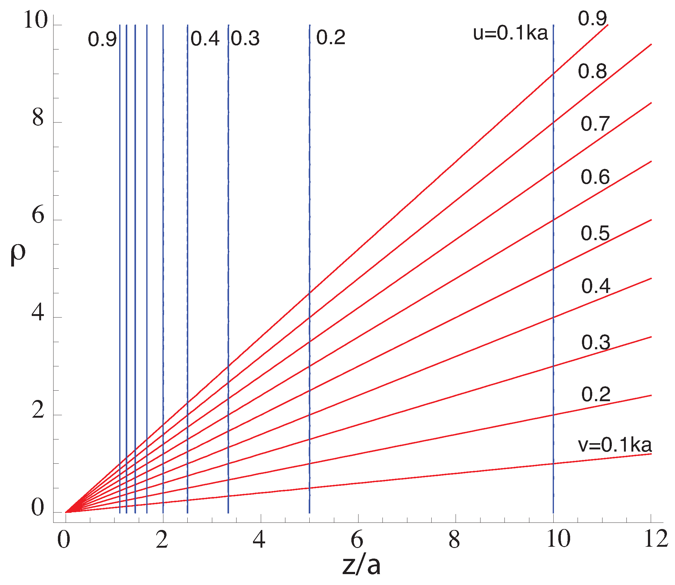
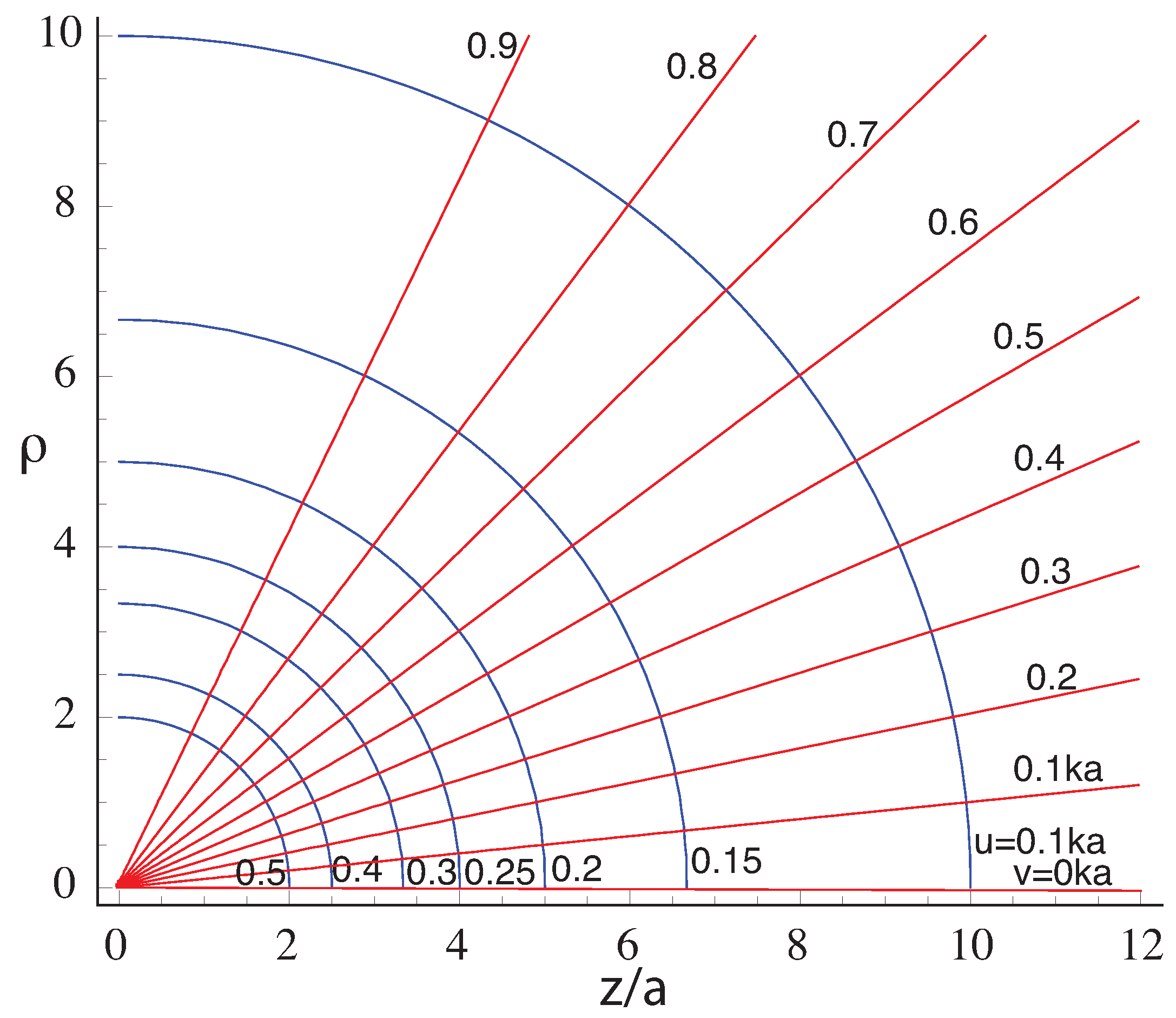

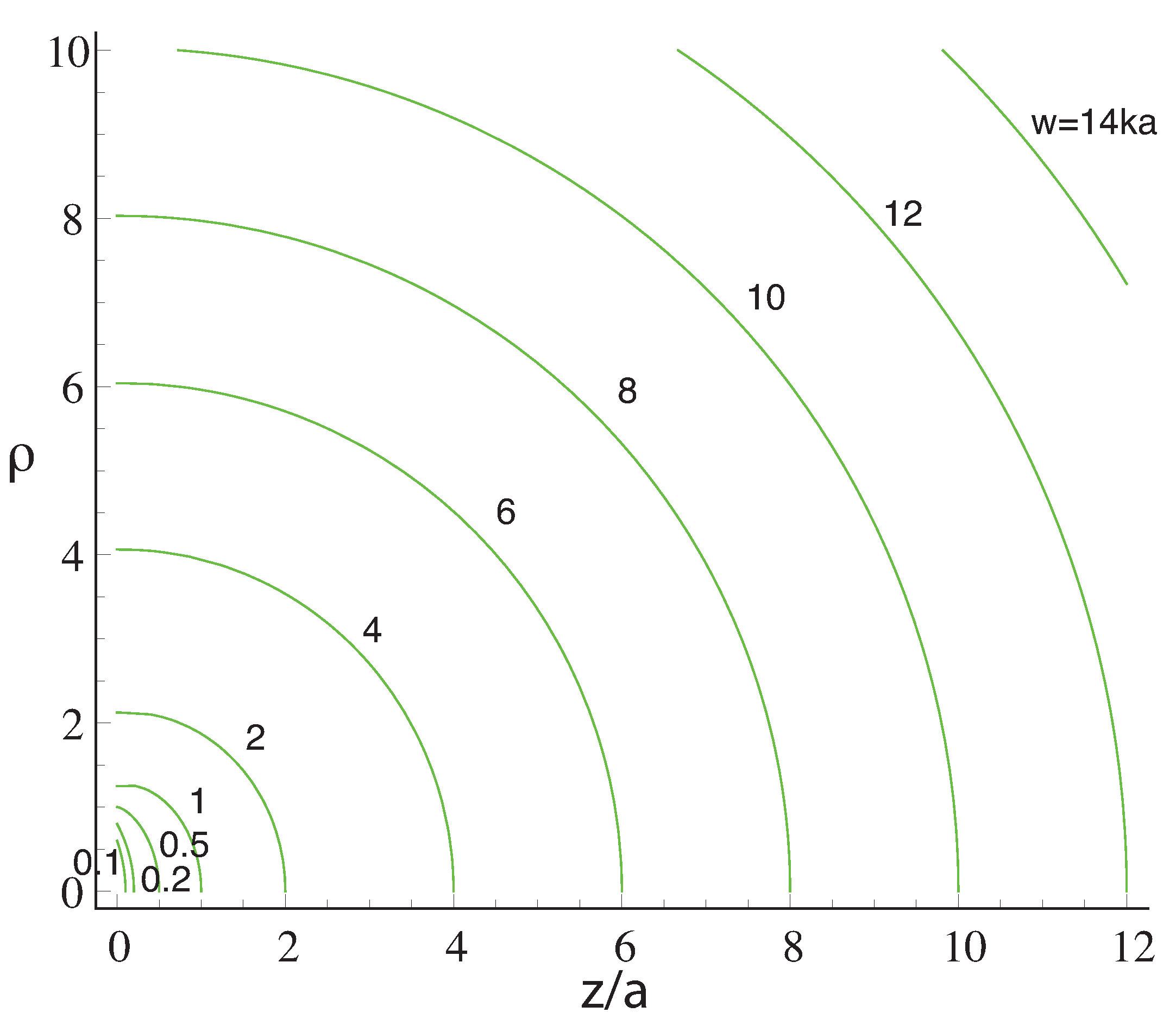
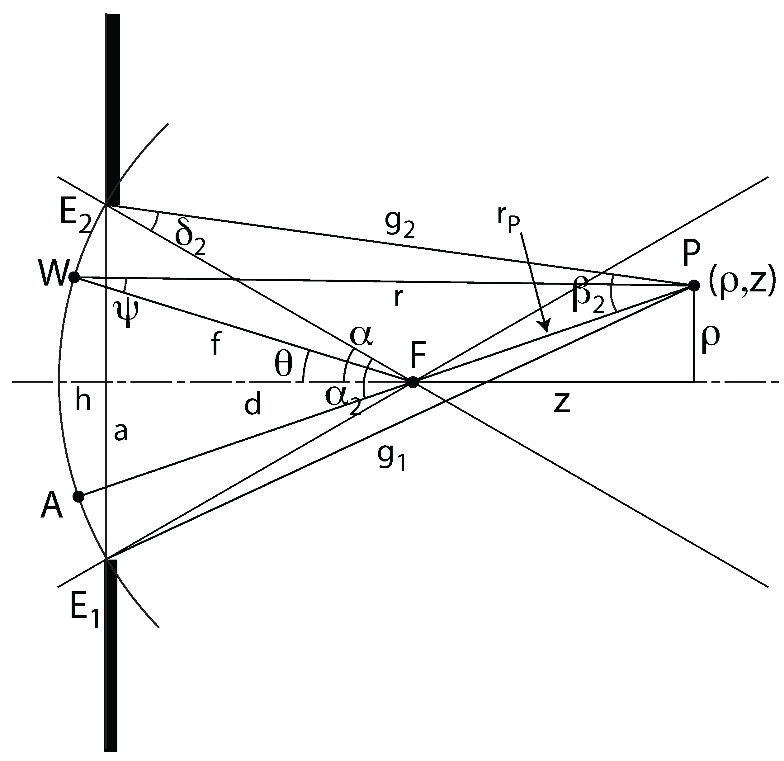
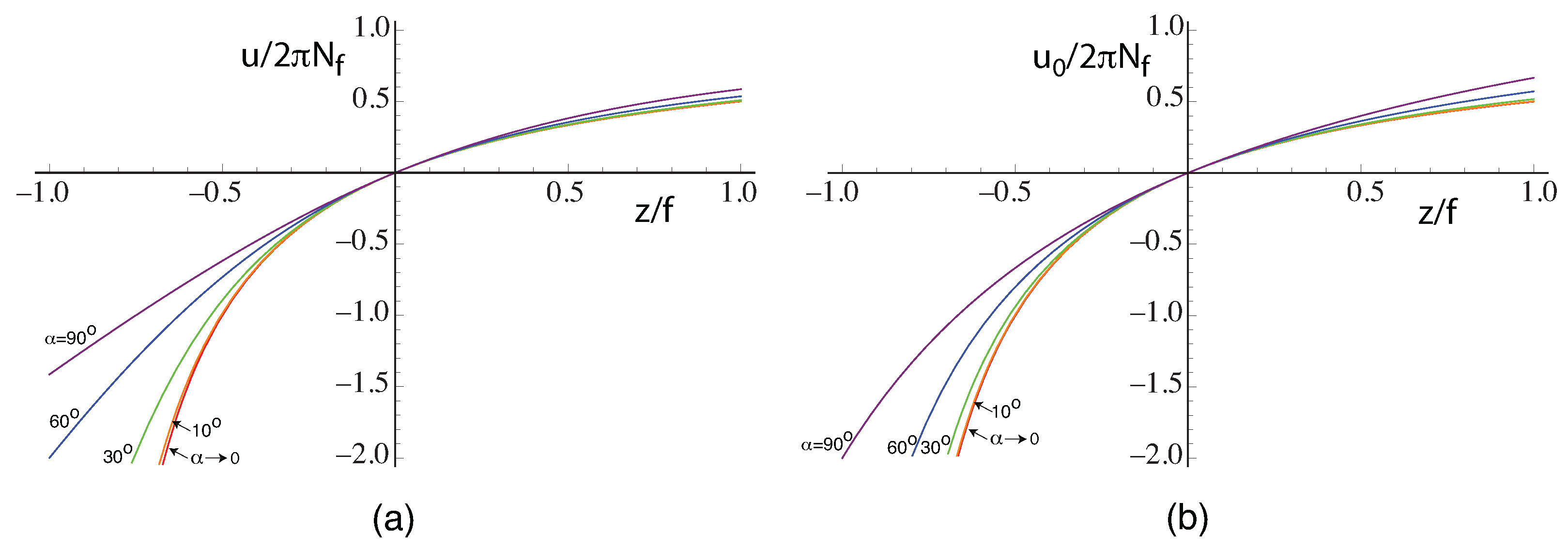
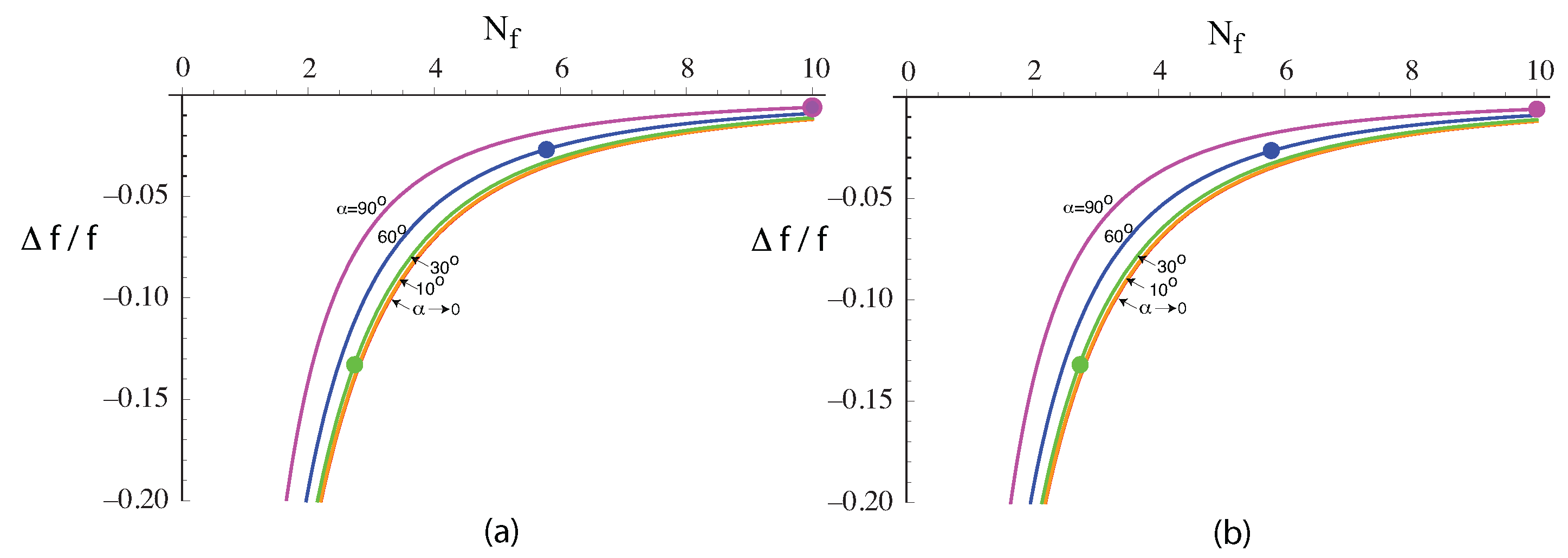
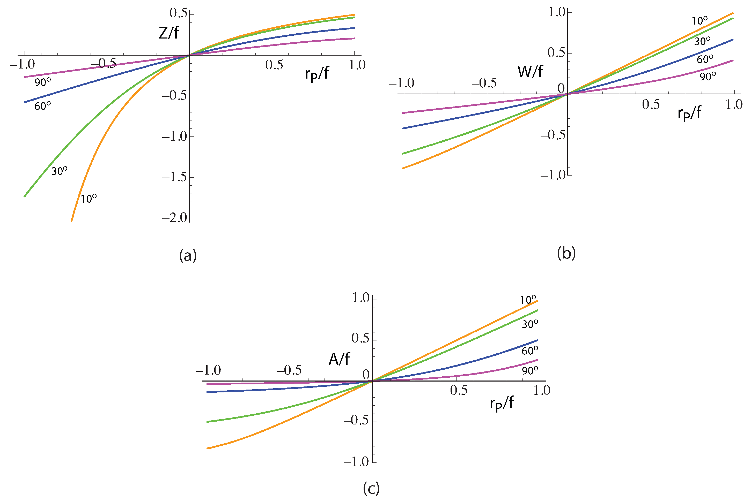
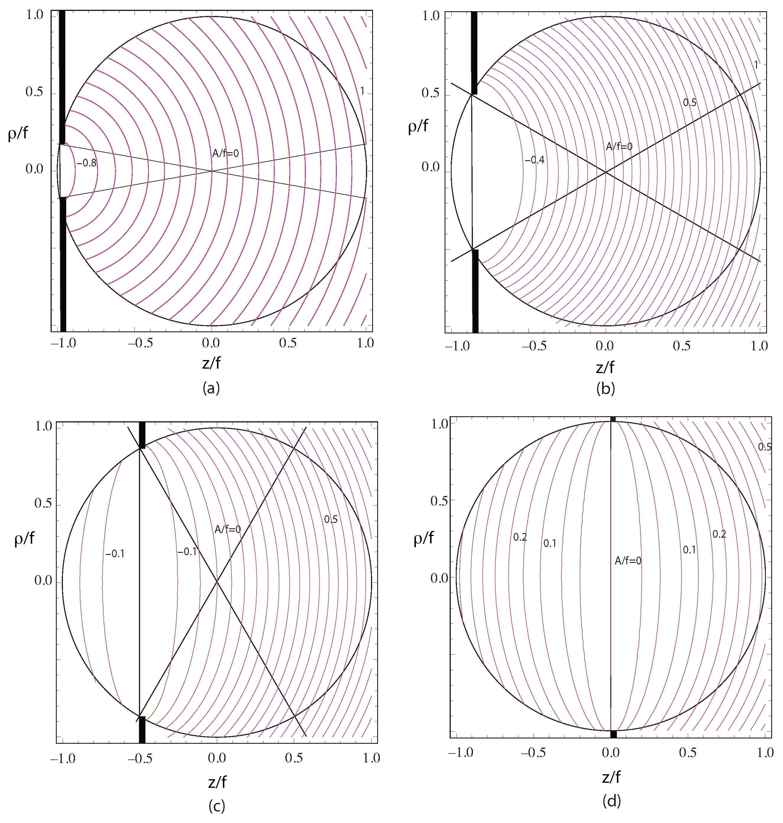
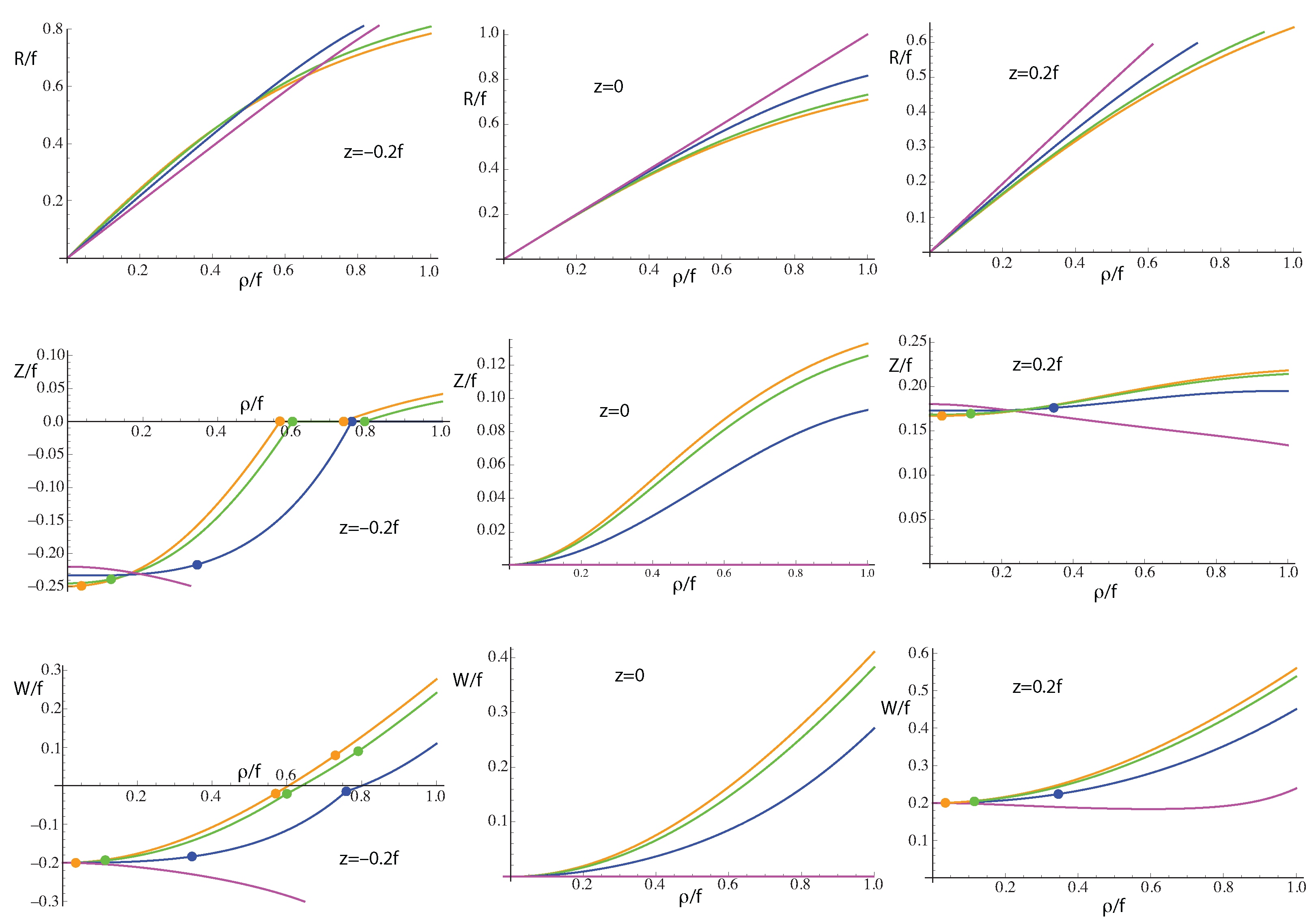
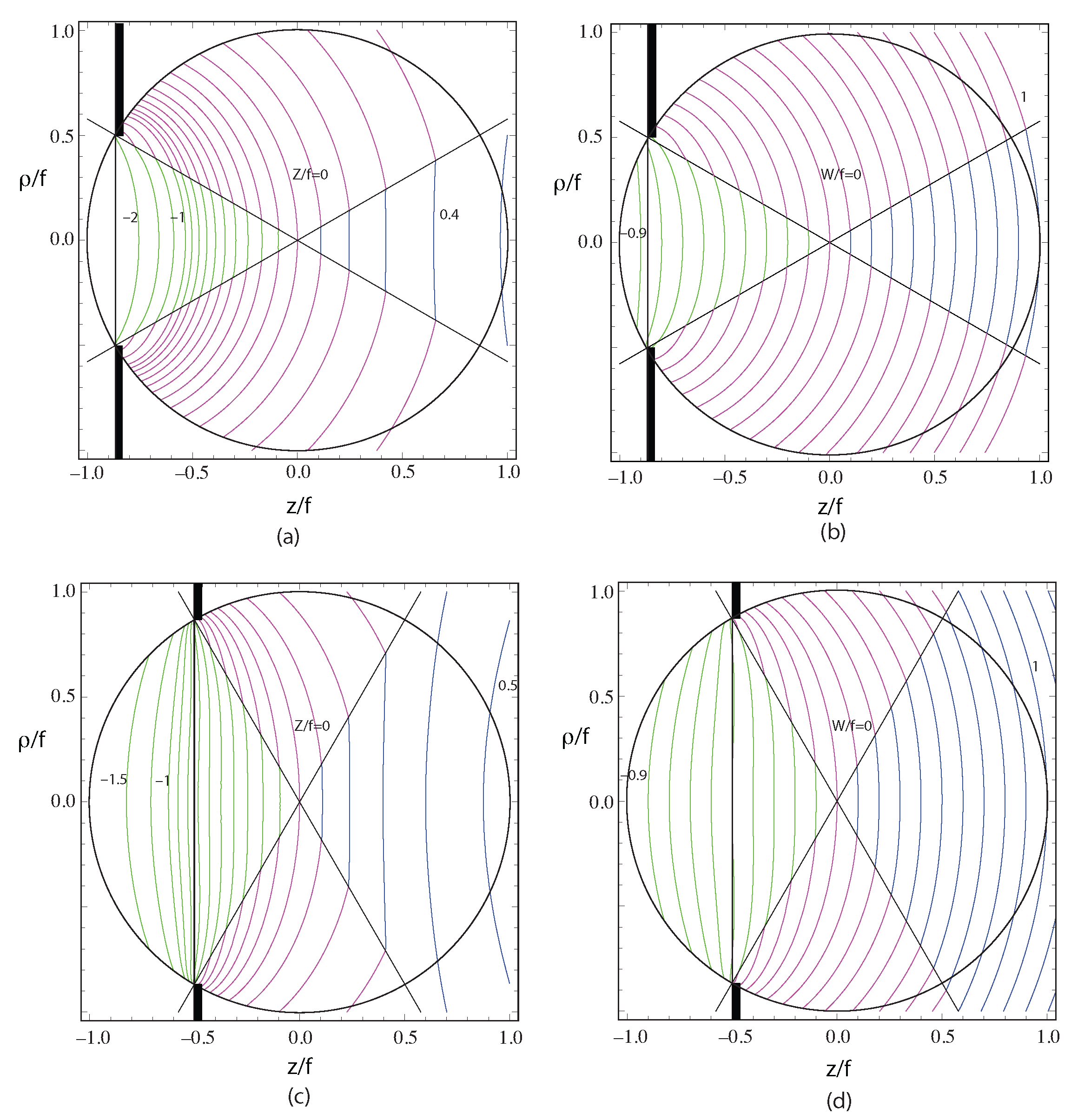
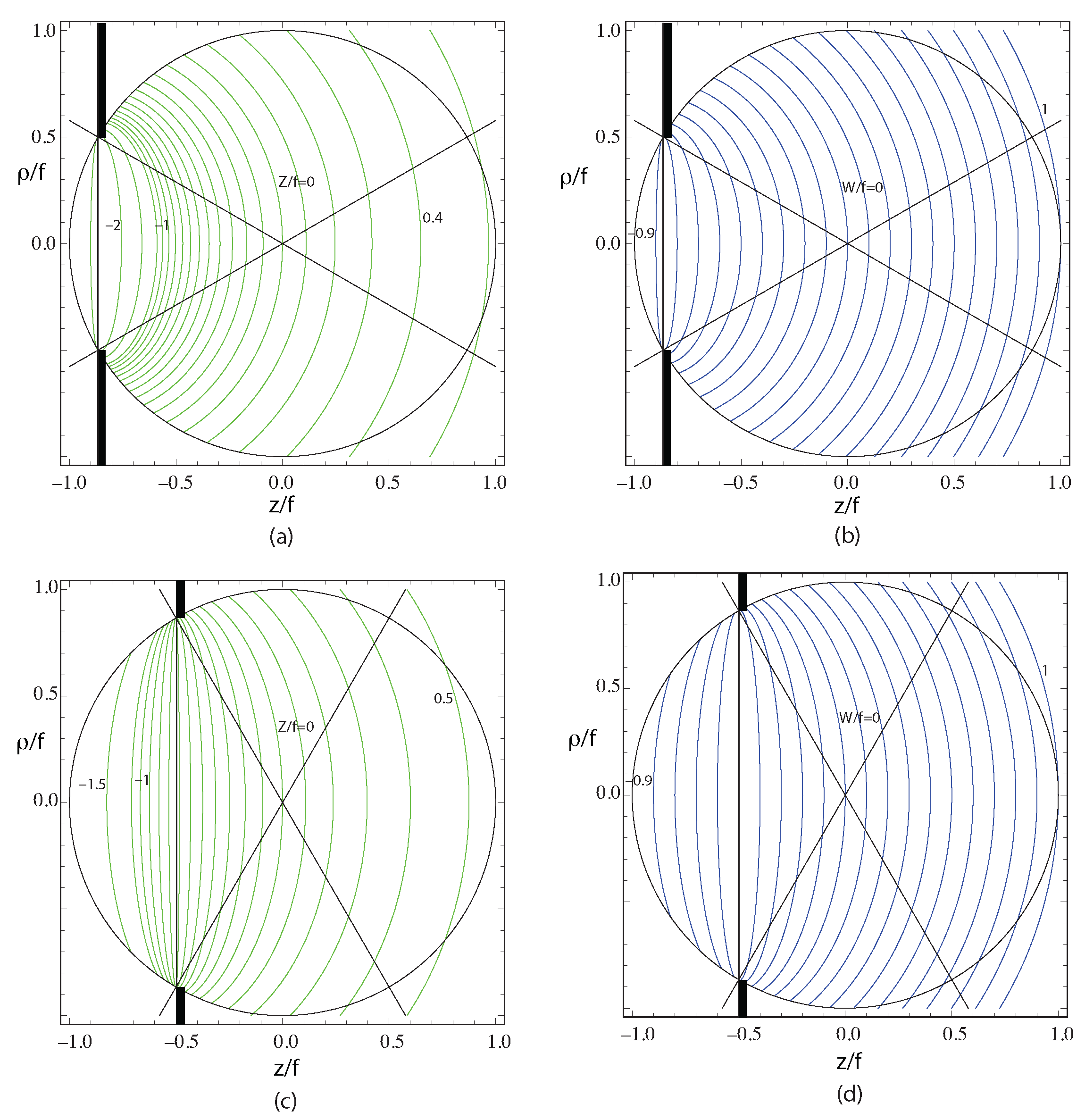
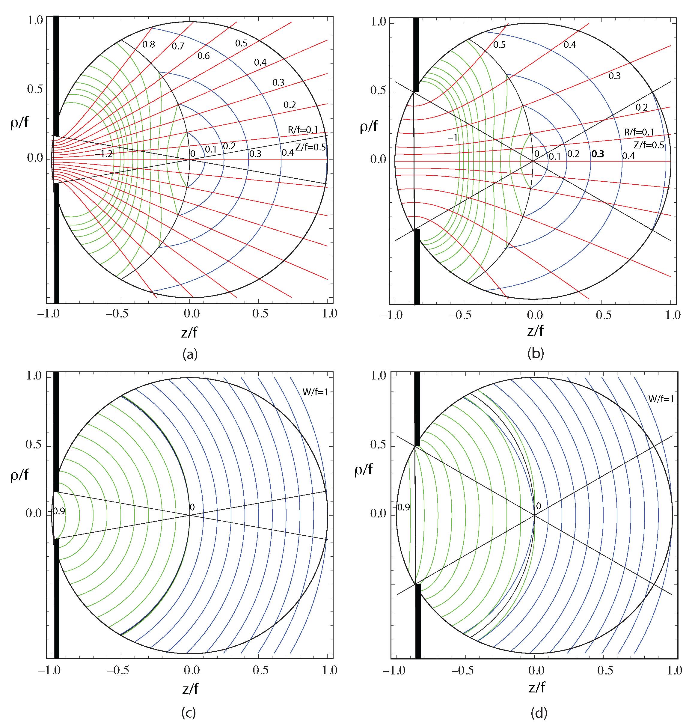
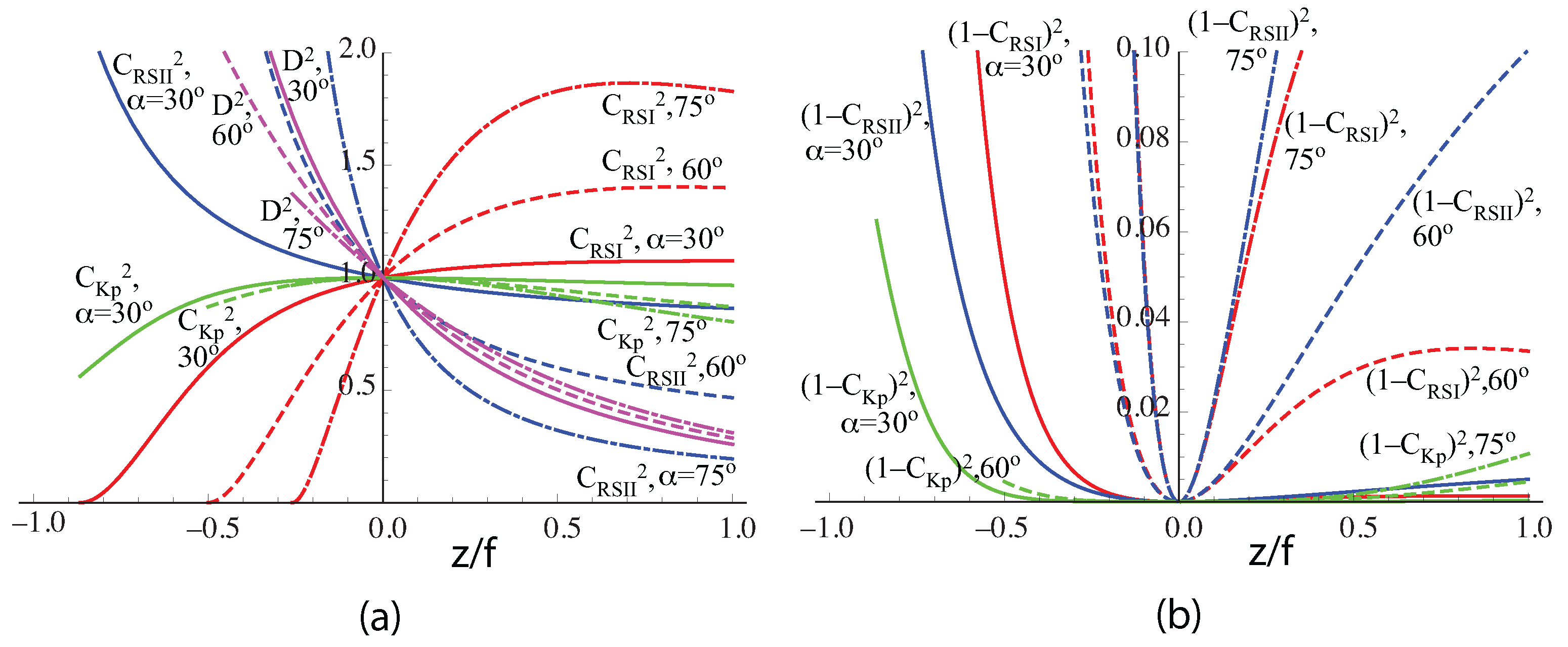
Disclaimer/Publisher’s Note: The statements, opinions and data contained in all publications are solely those of the individual author(s) and contributor(s) and not of MDPI and/or the editor(s). MDPI and/or the editor(s) disclaim responsibility for any injury to people or property resulting from any ideas, methods, instructions or products referred to in the content. |
© 2024 by the author. Licensee MDPI, Basel, Switzerland. This article is an open access article distributed under the terms and conditions of the Creative Commons Attribution (CC BY) license (https://creativecommons.org/licenses/by/4.0/).