Computational Optical Scanning Holography


Abstract
1. Introduction
2. Systems
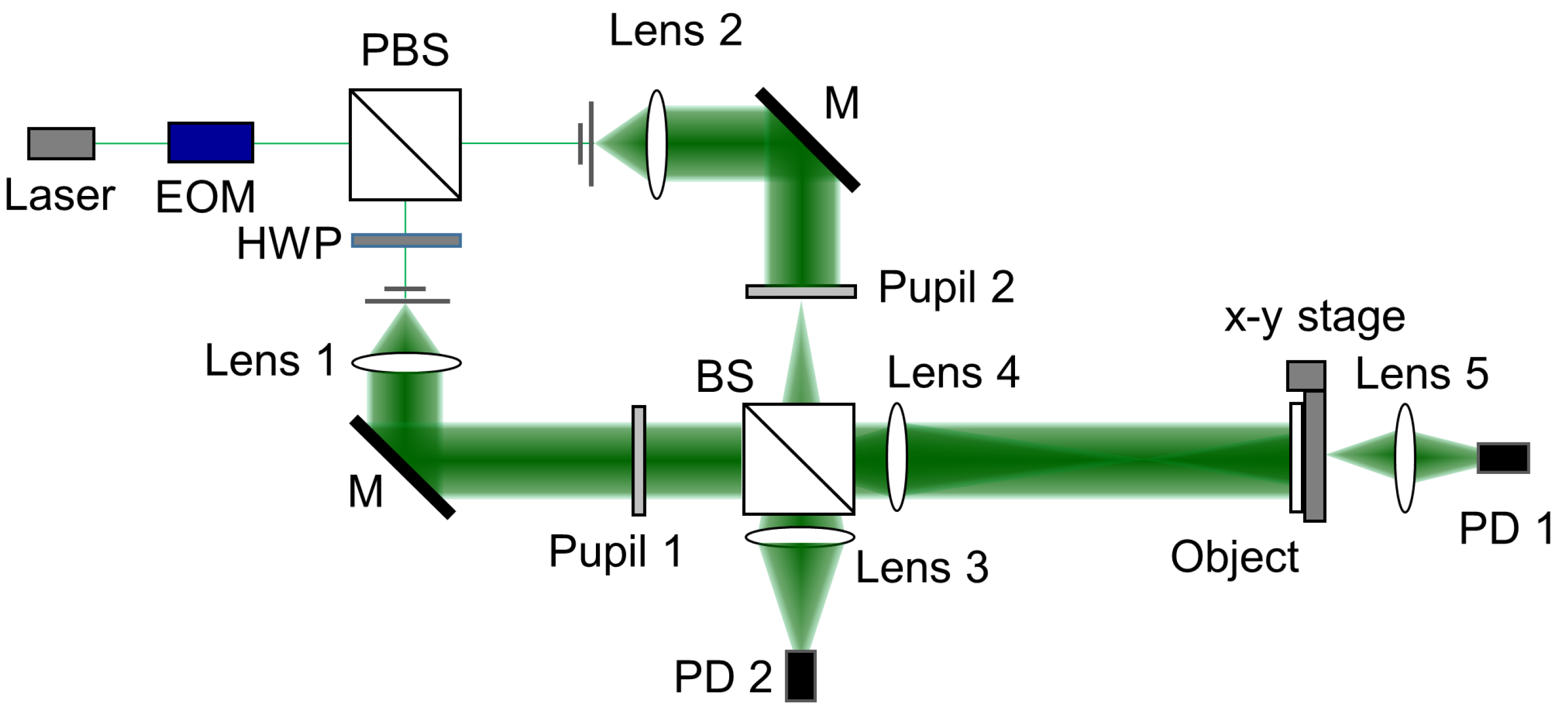
2.1. Basic Concept of Conventional OSH
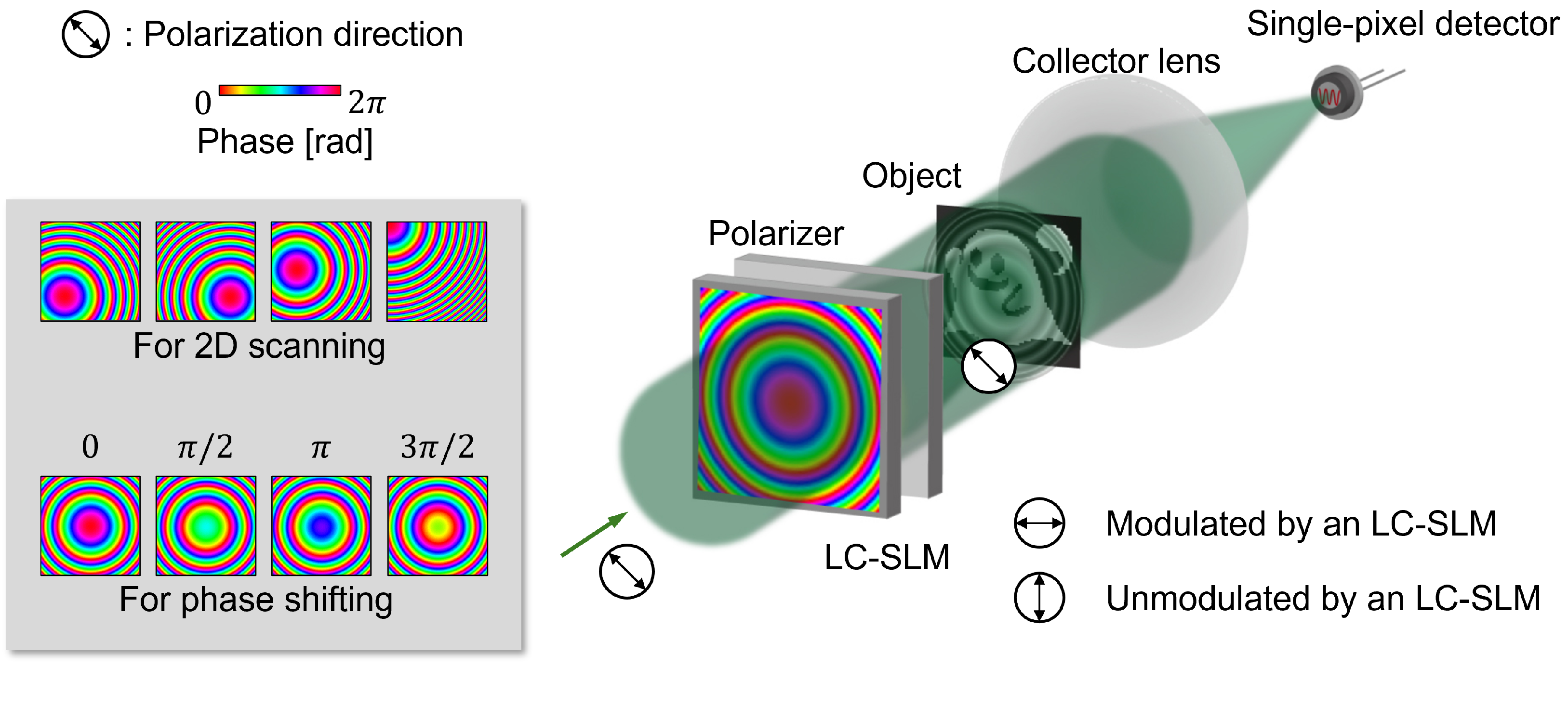
2.2. Motionless OSH
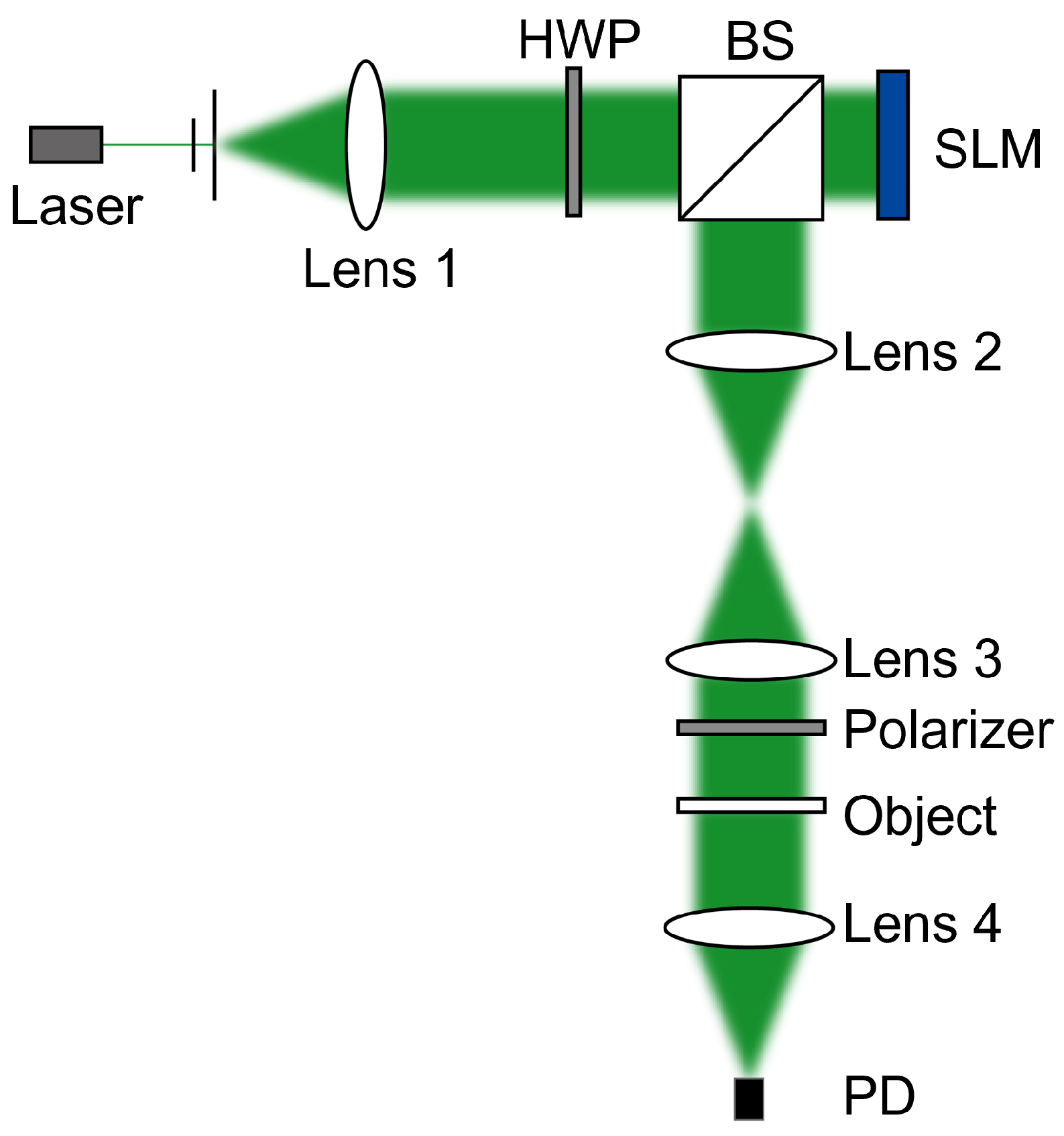
2.3. Interferenceless OSH
2.4. Comparison of OSH and COSH
3. Analysis Methods
3.1. Spatially Divided Phase-Shifting Method
3.2. Two-Step Spatially Divided Phase-Shifting Method
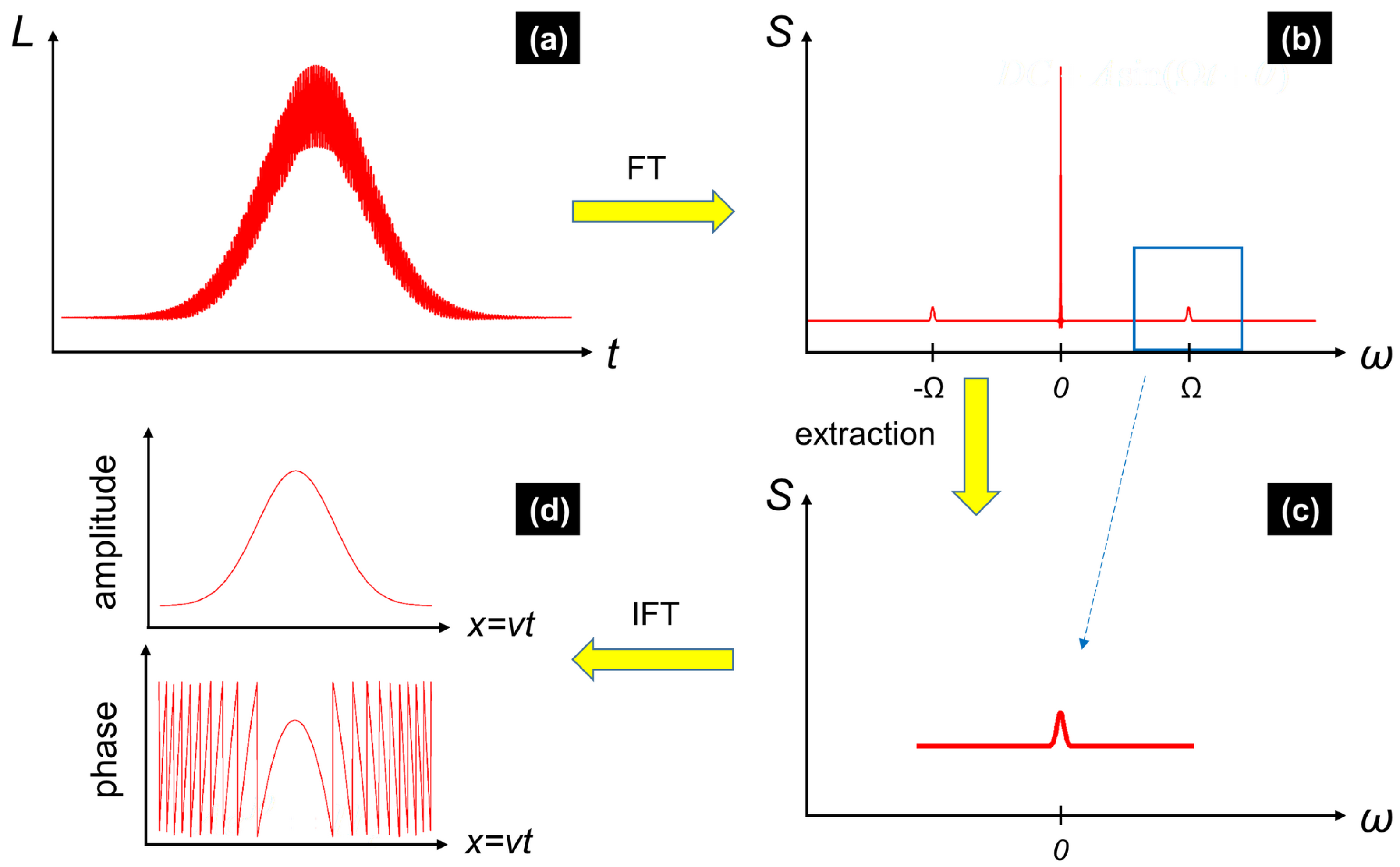
3.3. Digital Spatial–Temporal Demodulation
4. Applications
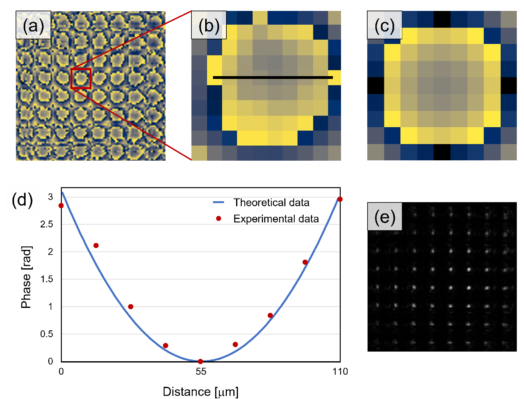
4.1. Quantitative Phase Imaging
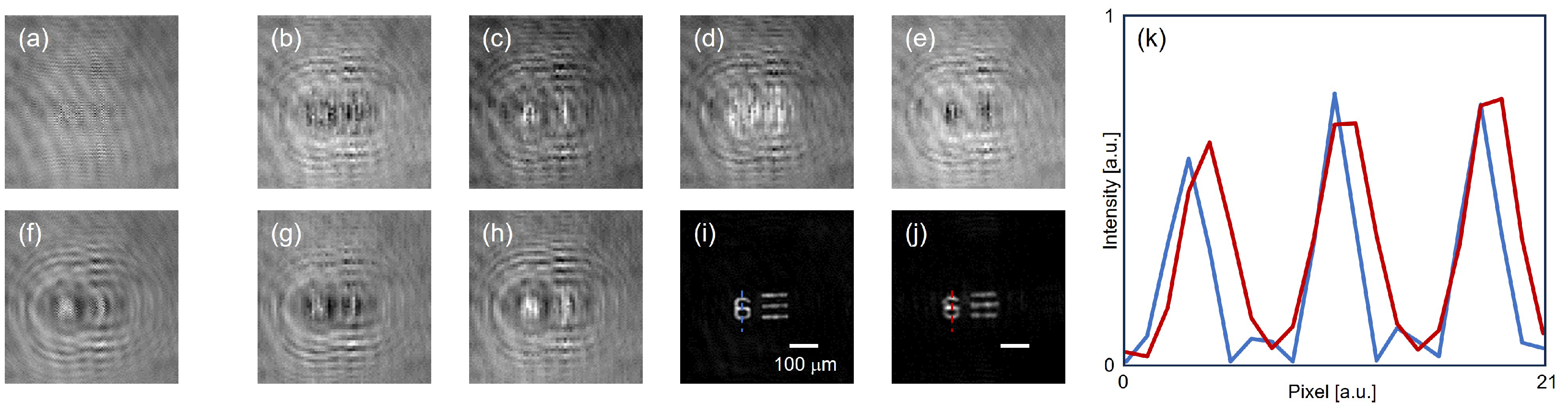
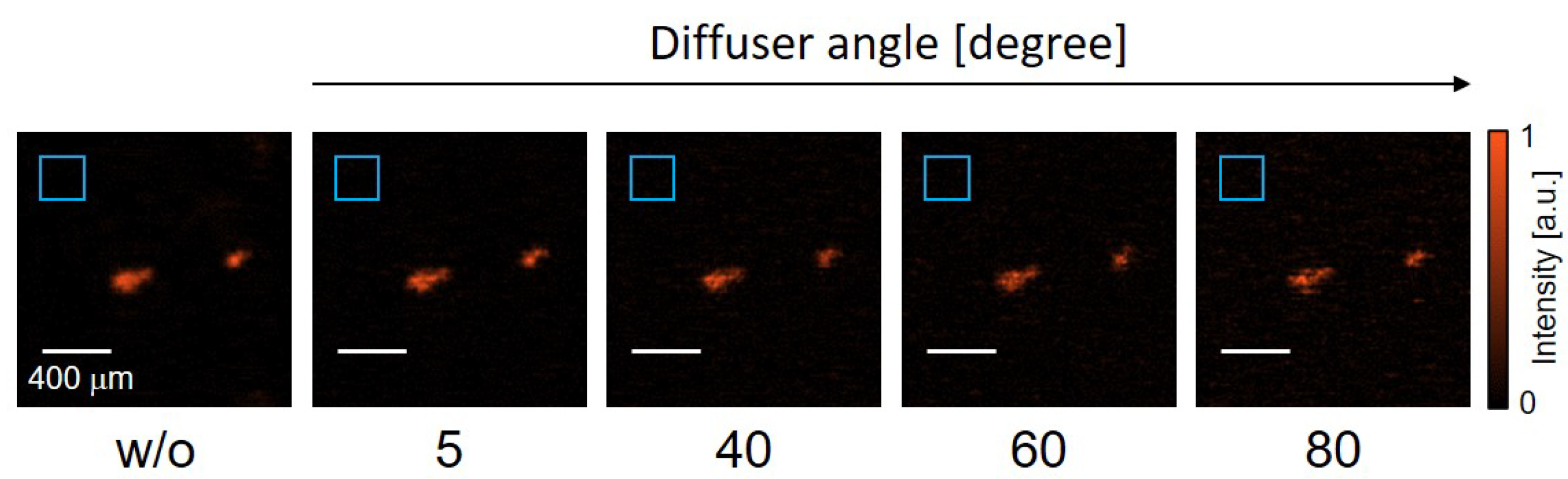
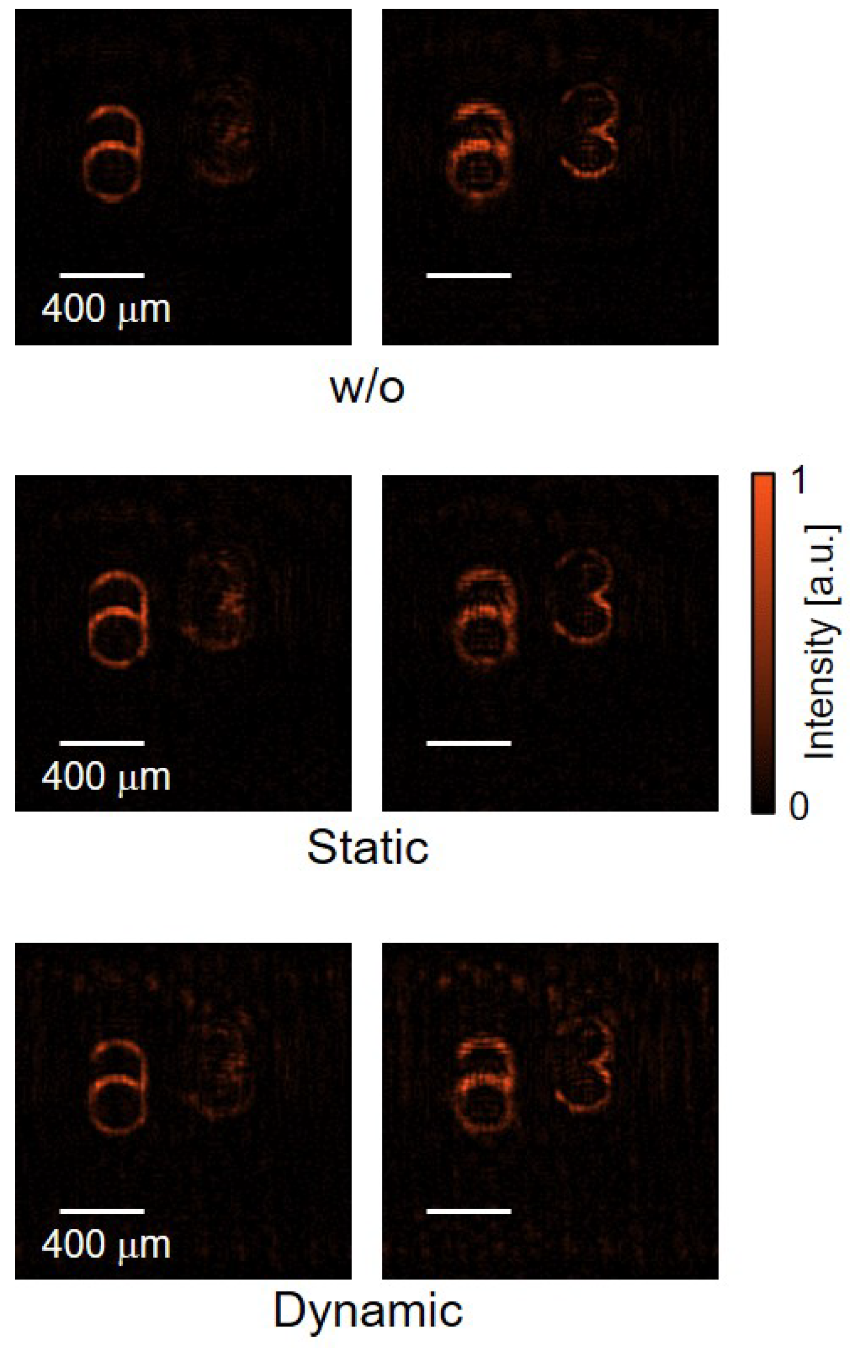
4.2. Imaging through Scattering Media
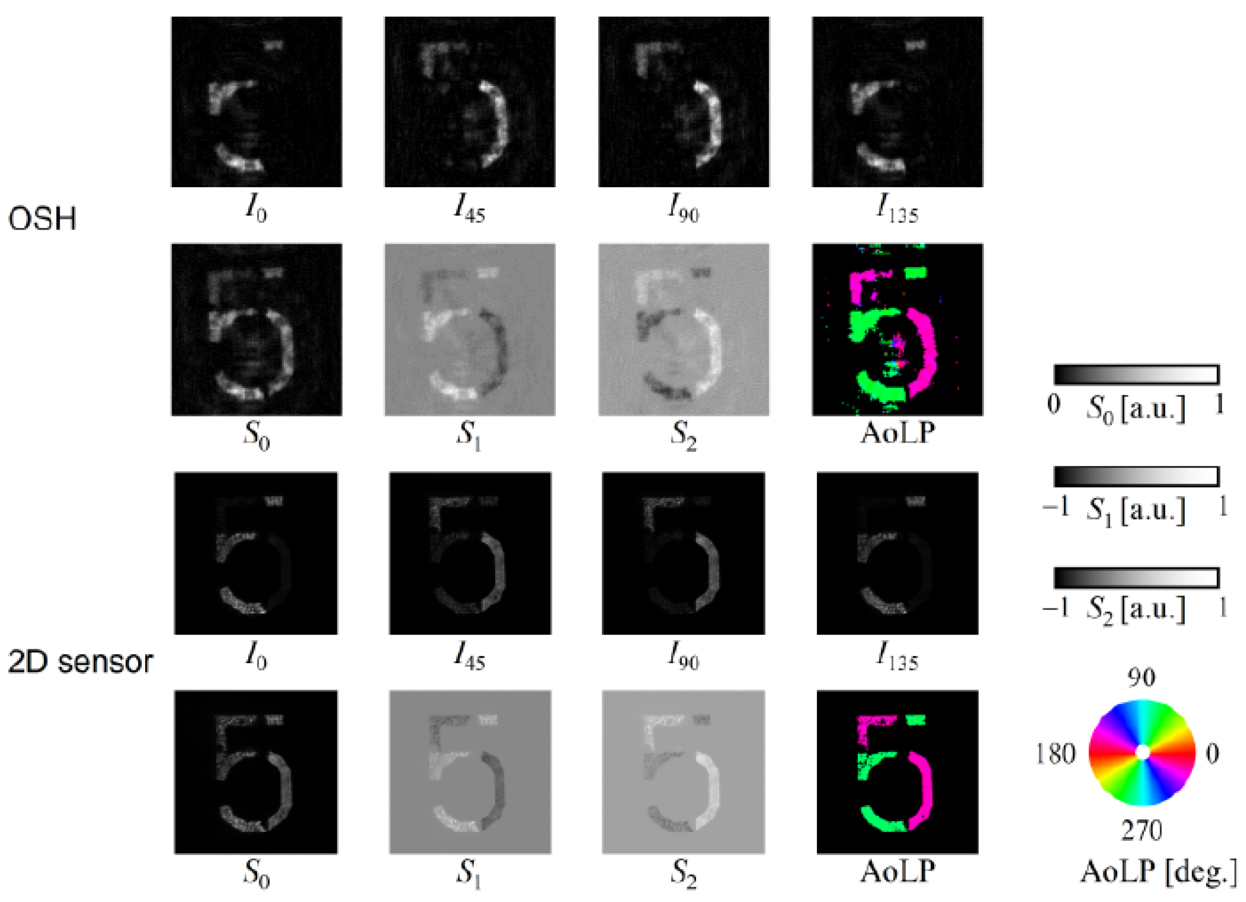
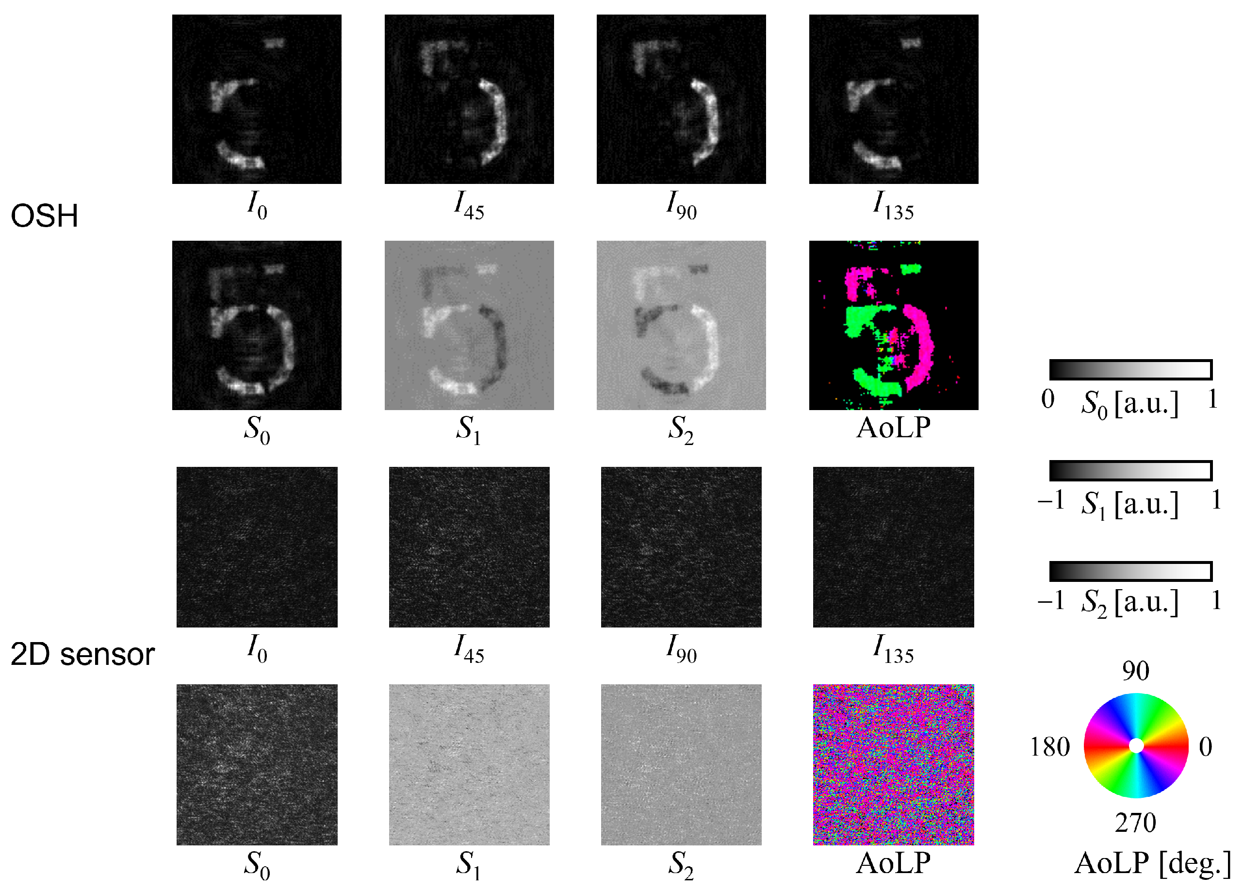
4.3. Polarization Imaging
5. Conclusions
Author Contributions
Funding
Institutional Review Board Statement
Informed Consent Statement
Data Availability Statement
Conflicts of Interest
Abbreviations
| OSH | Optical scanning holography |
| MOSH | Motionless optical scanning holography |
| IOSH | Interferenceless optical scanning holography |
| COSH | Computational optical scanning holography |
| SLM | Spatial light modulator |
| GI | Ghost imaging |
| CGI | Computational ghost imaging |
| HTI | Hadamard transform imaging |
| FSI | Fourier single-pixel imaging |
| IDH | Incoherent digital holography |
| CV | Coefficient of variance |
| SDPS | Spatially divided phase shifting |
| SBP | Space–bandwidth product |
References
- Mait, J.N.; Euliss, G.W.; Athale, R.A. Computational imaging. Adv. Opt. Photon. 2018, 10, 409–483. [Google Scholar] [CrossRef]
- Gibson, G.M.; Johnson, S.D.; Padgett, M.J. Single-pixel imaging 12 years on: A review. Opt. Express 2020, 28, 28190–28208. [Google Scholar] [CrossRef] [PubMed]
- Radwell, N.; Mitchell, K.J.; Gibson, G.M.; Edgar, M.P.; Bowman, R.; Padgett, M.J. Single-pixel infrared and visible microscope. Optica 2014, 1, 285–289. [Google Scholar] [CrossRef]
- Yu, H.; Lu, R.; Han, S.; Xie, H.; Du, G.; Xiao, T.; Zhu, D. Fourier-Transform Ghost Imaging with Hard X Rays. Phys. Rev. Lett. 2016, 117, 113901. [Google Scholar] [CrossRef] [PubMed]
- Gibson, G.M.; Sun, B.; Edgar, M.P.; Phillips, D.B.; Hempler, N.; Maker, G.T.; Malcolm, G.P.A.; Padgett, M.J. Real-time imaging of methane gas leaks using a single-pixel camera. Opt. Express 2017, 25, 2998–3005. [Google Scholar] [CrossRef] [PubMed]
- Vallés, A.; He, J.; Ohno, S.; Omatsu, T.; Miyamoto, K. Broadband high-resolution terahertz single-pixel imaging. Opt. Express 2020, 28, 28868–28881. [Google Scholar] [CrossRef] [PubMed]
- Olivieri, L.; Gongora, J.S.T.; Peters, L.; Cecconi, V.; Cutrona, A.; Tunesi, J.; Tucker, R.; Pasquazi, A.; Peccianti, M. Hyperspectral terahertz microscopy via nonlinear ghost imaging. Optica 2020, 7, 186–191. [Google Scholar] [CrossRef]
- Liu, X.; Shi, J.; Sun, L.; Li, Y.; Fan, J.; Zeng, G. Photon-limited single-pixel imaging. Opt. Express 2020, 28, 8132–8144. [Google Scholar] [CrossRef] [PubMed]
- Shibuya, K.; Araki, H.; Iwata, T. Photon-counting-based diffraction phase microscopy combined with single-pixel imaging. Jpn. J. Appl. Phys. 2018, 57, 042501. [Google Scholar] [CrossRef]
- Tajahuerce, E.; Durán, V.; Clemente, P.; Irles, E.; Soldevila, F.; Andrés, P.; Lancis, J. Image transmission through dynamic scattering media by single-pixel photodetection. Opt. Express 2014, 22, 16945–16955. [Google Scholar] [CrossRef]
- Yang, X.; Liu, Y.; Mou, X.; Hu, T.; Yuan, F.; Cheng, E. Imaging in turbid water based on a Hadamard single-pixel imaging system. Opt. Express 2021, 29, 12010–12023. [Google Scholar] [CrossRef] [PubMed]
- Pittman, T.B.; Shih, Y.H.; Strekalov, D.V.; Sergienko, A.V. Optical imaging by means of two-photon quantum entanglement. Phys. Rev. A 1995, 52, R3429–R3432. [Google Scholar] [CrossRef] [PubMed]
- Shapiro, J.H. Computational ghost imaging. Phys. Rev. A 2008, 78, 061802. [Google Scholar] [CrossRef]
- Pratt, W.; Kane, J.; Andrews, H. Hadamard transform image coding. Proc. IEEE 1969, 57, 58–68. [Google Scholar] [CrossRef]
- Zhang, Z.; Ma, X.; Zhong, J. Single-pixel imaging by means of Fourier spectrum acquisition. Nat. Commun. 2015, 6, 6225. [Google Scholar] [CrossRef] [PubMed]
- Poon, T.C.; Korpel, A. Optical transfer function of an acousto-optic heterodyning image processor. Opt. Lett. 1979, 4, 317. [Google Scholar] [CrossRef] [PubMed]
- Poon, T.C. Optical Scanning Holography with MATLAB®; Springer: Berlin/Heidelberg, Germany, 2007. [Google Scholar] [CrossRef]
- Kim, H.; Kim, Y.S.; Kim, T. Full-color optical scanning holography with common red, green, and blue channels [Invited]. Appl. Opt. 2016, 55, A17–A21. [Google Scholar] [CrossRef] [PubMed]
- Xin, Z.; Dobson, K.; Shinoda, Y.; Poon, T.C. Sectional image reconstruction in optical scanning holography using a random-phase pupil. Opt. Lett. 2010, 35, 2934–2936. [Google Scholar] [CrossRef] [PubMed]
- Wu, X.L.; Zhou, X.; Wang, Q.H.; Jiang, Y.F.; Xiao, C.J.; Dobson, K.; Poon, T.C. Deviation influences on sectional image reconstruction in optical scanning holography using a random-phase pupil. Appl. Opt. 2013, 52, A360–A366. [Google Scholar] [CrossRef]
- Ou, H.; Poon, T.C.; Wong, K.K.Y.; Lam, E.Y. Enhanced depth resolution in optical scanning holography using a configurable pupil. Photon. Res. 2014, 2, 64–70. [Google Scholar] [CrossRef][Green Version]
- Zhang, Y.; Wang, R.; Tsang, P.; Poon, T.C. Sectioning with edge extraction in optical incoherent imaging processing. OSA Contin. 2020, 3, 698–708. [Google Scholar] [CrossRef]
- Liu, J.P.; Wang, S.Y. Stereo-Lighting Reconstruction of Optical Scanning Holography. IEEE Trans. Ind. Informatics 2016, 12, 1664–1669. [Google Scholar] [CrossRef]
- Pan, Y.; Jia, W.; Yu, J.; Dobson, K.; Zhou, C.; Wang, Y.; Poon, T.C. Edge extraction using a time-varying vortex beam in incoherent digital holography. Opt. Lett. 2014, 39, 4176–4179. [Google Scholar] [CrossRef] [PubMed]
- Ou, H.; Wu, Y.; Lam, E.Y.; Wang, B.Z. Axial localization using time reversal multiple signal classification in optical scanning holography. Opt. Express 2018, 26, 3756–3771. [Google Scholar] [CrossRef]
- Chang, X.; Yan, A.; Zhang, H. Ciphertext-only attack on optical scanning cryptography. Opt. Lasers Eng. 2020, 126, 105901. [Google Scholar] [CrossRef]
- Ren, Z.; Lam, E.Y. Super-resolution imaging in optical scanning holography using structured illumination. In Proceedings of the Holography, Diffractive Optics, and Applications VII, Beijing, China, 12–14 October 2016; Sheng, Y., Yu, C., Zhou, C., Eds.; International Society for Optics and Photonics, SPIE: Bellingham, WA, USA, 2016; Volume 10022, p. 1002203. [Google Scholar] [CrossRef]
- Chen, N.; Ren, Z.; Ou, H.; Lam, E.Y. Resolution enhancement of optical scanning holography with a spiral modulated point spread function. Photon. Res. 2016, 4, 1–6. [Google Scholar] [CrossRef]
- Kim, T.; Poon, T.C.; Indebetouw, G.J.M. Depth detection and image recovery in remote sensing by optical scanning holography. Opt. Eng. 2002, 41, 1331–1338. [Google Scholar] [CrossRef]
- Liu, J.P.; Tahara, T.; Hayasaki, Y.; Poon, T.C. Incoherent Digital Holography: A Review. Appl. Sci. 2018, 8, 143. [Google Scholar] [CrossRef]
- Yoneda, N.; Ipus, E.; Ordóñez, L.; Lenz, A.J.M.; Martínez-León, L.; Matoba, O.; Tajahuerce, E. Videography based on computational optical scanning holography. In Proceedings of the Optica Imaging Congress (3D, COSI, DH, FLatOptics, IS, pcAOP), Boston, MA ,USA, 14–17 August 2023; Optica Publishing Group: Washington, DC, USA, 2023; p. HM4C.8. [Google Scholar] [CrossRef]
- Yu, H.; Kim, Y.; Yang, D.; Seo, W.; Kim, Y.; Hong, J.Y.; Song, H.; Sung, G.; Sung, Y.; Min, S.W.; et al. Deep learning-based incoherent holographic camera enabling acquisition of real-world holograms for holographic streaming system. Nat. Commun. 2023, 14, 3534. [Google Scholar] [CrossRef] [PubMed]
- Muroi, T.; Nobukawa, T.; Katano, Y.; Hagiwara, K. Capturing videos at 60 frames per second using incoherent digital holography. Opt. Contin. 2023, 2, 2409–2420. [Google Scholar] [CrossRef]
- Tahara, T.; Shimobaba, T. High-speed phase-shifting incoherent digital holography (invited). Appl. Phys. B 2023, 129, 96. [Google Scholar] [CrossRef]
- Tsang, P.W.M.; Liu, J.P.; Poon, T.C. Compressive optical scanning holography. Optica 2015, 2, 476–483. [Google Scholar] [CrossRef]
- Chan, A.C.S.; Tsia, K.K.; Lam, E.Y. Subsampled scanning holographic imaging (SuSHI) for fast, non-adaptive recording of three-dimensional objects. Optica 2016, 3, 911–917. [Google Scholar] [CrossRef]
- Tsang, P.W.M.; Poon, T.C.; Liu, J.P. Adaptive Optical Scanning Holography. Sci. Rep. 2016, 6, 21636. [Google Scholar] [CrossRef] [PubMed]
- Tsang, P.W.M.; Poon, T.C.; Liu, J.P.; Kim, T.; Kim, Y.S. Low Complexity Compression and Speed Enhancement for Optical Scanning Holography. Sci. Rep. 2016, 6, 34724. [Google Scholar] [CrossRef]
- Indebetouw, G.; Klysubun, P.; Kim, T.; Poon, T.C. Imaging properties of scanning holographic microscopy. J. Opt. Soc. Am. A 2000, 17, 380–390. [Google Scholar] [CrossRef]
- Indebetouw, G.; Tada, Y.; Leacock, J. Quantitative phase imaging with scanning holographic microscopy: An experimental assesment. Biomed. Eng. Online 2006, 5, 63. [Google Scholar] [CrossRef] [PubMed]
- Liu, J.P. Spatial coherence analysis for optical scanning holography. Appl. Opt. 2015, 54, A59–A66. [Google Scholar] [CrossRef] [PubMed]
- Liu, J.P.; Guo, C.H.; Hsiao, W.J.; Poon, T.C.; Tsang, P. Coherence experiments in single-pixel digital holography. Opt. Lett. 2015, 40, 2366–2369. [Google Scholar] [CrossRef]
- Kim, T.; Kim, T. Coaxial scanning holography. Opt. Lett. 2020, 45, 2046–2049. [Google Scholar] [CrossRef]
- Tsai, C.M.; Sie, H.Y.; Poon, T.C.; Liu, J.P. Optical scanning holography with a polarization directed flat lens. Appl. Opt. 2021, 60, B113–B118. [Google Scholar] [CrossRef] [PubMed]
- Yoneda, N.; Saita, Y.; Nomura, T. Motionless optical scanning holography. Opt. Lett. 2020, 45, 3184–3187. [Google Scholar] [CrossRef] [PubMed]
- Liu, J.P.; Tsai, C.M.; Poon, T.C.; Tsang, P.; Zhang, Y. Three-dimensional imaging by interferenceless optical scanning holography. Opt. Lasers Eng. 2022, 158, 107183. [Google Scholar] [CrossRef]
- Shinoda, Y.; Liu, J.P.; Chung, P.S.; Dobson, K.; Zhou, X.; Poon, T.C. Three-dimensional complex image coding using a circular Dammann grating. Appl. Opt. 2011, 50, B38–B45. [Google Scholar] [CrossRef] [PubMed]
- Liu, J.P.; Lee, C.C.; Lo, Y.H.; Luo, D.Z. Vertical-bandwidth-limited digital holography. Opt. Lett. 2012, 37, 2574–2576. [Google Scholar] [CrossRef] [PubMed]
- Zhang, L.Z.; Zhou, X.; Wang, D.; Li, N.N.; Bai, X.; Wang, Q.H. Multiple-image encryption based on optical scanning holography using orthogonal compressive sensing and random phase mask. Opt. Eng. 2020, 59, 102411. [Google Scholar] [CrossRef]
- Zhang, Y.; Poon, T.C.; Tsang, P.W.M.; Wang, R.; Wang, L. Review on Feature Extraction for 3-D Incoherent Image Processing Using Optical Scanning Holography. IEEE Trans. Ind. Inform. 2019, 15, 6146–6154. [Google Scholar] [CrossRef]
- Swoger, J.; Martinez-Corral, M.; Huisken, J.; Stelzer, E.H.K. Optical scanning holography as a technique for high-resolution three-dimensional biological microscopy. J. Opt. Soc. Am. A 2002, 19, 1910–1918. [Google Scholar] [CrossRef] [PubMed]
- Rosen, J.; Brooker, G. Digital spatially incoherent Fresnel holography. Opt. Lett. 2007, 32, 912–914. [Google Scholar] [CrossRef]
- Takasaki, H.; Yoshino, Y. Polarization Interferometer. Appl. Opt. 1969, 8, 2344–2345. [Google Scholar] [CrossRef]
- Yoneda, N.; Saita, Y.; Nomura, T. Spatially divided phase-shifting motionless optical scanning holography. OSA Contin. 2020, 3, 3523–3535. [Google Scholar] [CrossRef]
- Tsang, P.; Poon, T.C. Non-diffractive Optical Scanning Holography for Hologram Acquisition. In Proceedings of the Digital Holography and Three-Dimensional Imaging 2019, Bordeaux, France, 19–23 May 2019; Optica Publishing Group: Washington, DC, USA, 2019; p. Th1B.6. [Google Scholar] [CrossRef]
- Nomura, T.; Shinomura, K. Generalized sequential four-step phase-shifting color digital holography. Appl. Opt. 2017, 56, 6851–6854. [Google Scholar] [CrossRef]
- Awatsuji, Y.; Sasada, M.; Kubota, T. Parallel quasi-phase-shifting digital holography. Appl. Phys. Lett. 2004, 85, 1069–1071. [Google Scholar] [CrossRef]
- Awatsuji, Y.; Tahara, T.; Kaneko, A.; Koyama, T.; Nishio, K.; Ura, S.; Kubota, T.; Matoba, O. Parallel two-step phase-shifting digital holography. Appl. Opt. 2008, 47, D183–D189. [Google Scholar] [CrossRef]
- Tahara, T.; Ito, K.; Kakue, T.; Fujii, M.; Shimozato, Y.; Awatsuji, Y.; Nishio, K.; Ura, S.; Kubota, T.; Matoba, O. Parallel phase-shifting digital holographic microscopy. Biomed. Opt. Express 2010, 1, 610–616. [Google Scholar] [CrossRef]
- Yoneda, N.; Quan, X.; Matoba, O. Single-shot generalized Hanbury Brown & Twiss experiments using a polarization camera for target intensity reconstruction in scattering media. Opt. Lett. 2023, 48, 632–635. [Google Scholar] [CrossRef]
- Kakue, T.; Yonesaka, R.; Tahara, T.; Awatsuji, Y.; Nishio, K.; Ura, S.; Kubota, T.; Matoba, O. High-speed phase imaging by parallel phase-shifting digital holography. Opt. Lett. 2011, 36, 4131–4133. [Google Scholar] [CrossRef]
- Takase, Y.; Shimizu, K.; Mochida, S.; Inoue, T.; Nishio, K.; Rajput, S.K.; Matoba, O.; Xia, P.; Awatsuji, Y. High-speed imaging of the sound field by parallel phase-shifting digital holography. Appl. Opt. 2021, 60, A179–A187. [Google Scholar] [CrossRef]
- Yoneda, N.; Matoba, O. Two-Step Phase-Shifting Motionless Optical Scanning Holography. In Proceedings of the Imaging and Applied Optics Congress 2022 (3D, AOA, COSI, ISA, pcAOP), Vancouver, BC, Canada, 11–15 July 2022; Optica Publishing Group: Washington, DC, USA, 2022; p. 3F3A.7. [Google Scholar] [CrossRef]
- Yoneda, N.; Matoba, O. Spatially divided two-step phase-shifting method for computational optical scanning holography. J. Opt. 2023, 25, 124001. [Google Scholar] [CrossRef]
- Meng, X.F.; Cai, L.Z.; Xu, X.F.; Yang, X.L.; Shen, X.X.; Dong, G.Y.; Wang, Y.R. Two-step phase-shifting interferometry and its application in image encryption. Opt. Lett. 2006, 31, 1414–1416. [Google Scholar] [CrossRef]
- Liu, J.P.; Poon, T.C. Two-step-only quadrature phase-shifting digital holography. Opt. Lett. 2009, 34, 250–252. [Google Scholar] [CrossRef]
- Tahara, T.; Kozawa, Y.; Ishii, A.; Wakunami, K.; Ichihashi, Y.; Oi, R. Two-step phase-shifting interferometry for self-interference digital holography. Opt. Lett. 2021, 46, 669–672. [Google Scholar] [CrossRef]
- Poon, T.C.; Kim, T.; Indebetouw, G.; Schilling, B.W.; Wu, M.H.; Shinoda, K.; Suzuki, Y. Twin-image elimination experiments for three-dimensional images in optical scanning holography. Opt. Lett. 2000, 25, 215–217. [Google Scholar] [CrossRef]
- Indebetouw, G.; Zhong, W. Scanning holographic microscopy of three-dimensional fluorescent specimens. J. Opt. Soc. Am. A 2006, 23, 1699–1707. [Google Scholar] [CrossRef]
- Liu, J.P.; Luo, D.Z.; Lu, S.H. Spatial–temporal demodulation technique for heterodyne optical scanning holography. Opt. Lasers Eng. 2015, 68, 42–49. [Google Scholar] [CrossRef]
- Muñoz, V.H.F.; Arellano, N.I.T.; García, D.I.S.; García, A.M.; Zurita, G.R.; Lechuga, L.G. Measurement of mean thickness of transparent samples using simultaneous phase shifting interferometry with four interferograms. Appl. Opt. 2016, 55, 4047–4051. [Google Scholar] [CrossRef]
- Takabayashi, M.; Majeed, H.; Kajdacsy-Balla, A.; Popescu, G. Disorder strength measured by quantitative phase imaging as intrinsic cancer marker in fixed tissue biopsies. PLoS ONE 2018, 13, e0194320. [Google Scholar] [CrossRef]
- Choi, I.; Lee, K.; Park, Y. Compensation of aberration in quantitative phase imaging using lateral shifting and spiral phase integration. Opt. Express 2017, 25, 30771–30779. [Google Scholar] [CrossRef]
- Tamamitsu, M.; Toda, K.; Horisaki, R.; Ideguchi, T. Quantitative phase imaging with molecular vibrational sensitivity. Opt. Lett. 2019, 44, 3729–3732. [Google Scholar] [CrossRef]
- Ma, Y.; Dai, T.; Lei, Y.; Zheng, J.; Liu, M.; Sui, B.; Smith, Z.J.; Chu, K.; Kong, L.; Gao, P. Label-free imaging of intracellular organelle dynamics using flat-fielding quantitative phase contrast microscopy (FF-QPCM). Opt. Express 2022, 30, 9505–9520. [Google Scholar] [CrossRef]
- Yoneda, N.; Matoba, O.; Saita, Y.; Nomura, T. Quantitative phase imaging based on motionless optical scanning holography. Opt. Lett. 2023, 48, 5273–5276. [Google Scholar] [CrossRef]
- Rotter, S.; Gigan, S. Light fields in complex media: Mesoscopic scattering meets wave control. Rev. Mod. Phys. 2017, 89, 015005. [Google Scholar] [CrossRef]
- Popoff, S.M.; Lerosey, G.; Carminati, R.; Fink, M.; Boccara, A.C.; Gigan, S. Measuring the Transmission Matrix in Optics: An Approach to the Study and Control of Light Propagation in Disordered Media. Phys. Rev. Lett. 2010, 104, 100601. [Google Scholar] [CrossRef]
- Kim, M.; Choi, W.; Choi, Y.; Yoon, C.; Choi, W. Transmission matrix of a scattering medium and its applications in biophotonics. Opt. Express 2015, 23, 12648–12668. [Google Scholar] [CrossRef]
- Li, L.; Li, Q.; Sun, S.; Lin, H.Z.; Liu, W.T.; Chen, P.X. Imaging through scattering layers exceeding memory effect range with spatial-correlation-achieved point-spread-function. Opt. Lett. 2018, 43, 1670–1673. [Google Scholar] [CrossRef]
- Wu, T.; Dong, J.; Gigan, S. Non-invasive single-shot recovery of a point-spread function of a memory effect based scattering imaging system. Opt. Lett. 2020, 45, 5397–5400. [Google Scholar] [CrossRef]
- Bertolotti, J.; van Putten, E.G.; Blum, C.; Lagendijk, A.; Vos, W.L.; Mosk, A.P. Non-invasive imaging through opaque scattering layers. Nature 2012, 491, 232–234. [Google Scholar] [CrossRef]
- Liao, M.; Lu, D.; He, W.; Pedrini, G.; Osten, W.; Peng, X. Improving reconstruction of speckle correlation imaging by using a modified phase retrieval algorithm with the number of nonzero-pixels constraint. Appl. Opt. 2019, 58, 473–478. [Google Scholar] [CrossRef]
- Durán, V.; Soldevila, F.; Irles, E.; Clemente, P.; Tajahuerce, E.; Andrés, P.; Lancis, J. Compressive imaging in scattering media. Opt. Express 2015, 23, 14424–14433. [Google Scholar] [CrossRef]
- Martínez-León, L.; Clemente, P.; Mori, Y.; Climent, V.; Lancis, J.; Tajahuerce, E. Single-pixel digital holography with phase-encoded illumination. Opt. Express 2017, 25, 4975–4984. [Google Scholar] [CrossRef]
- Dutta, R.; Manzanera, S.; Gambín-Regadera, A.; Irles, E.; Tajahuerce, E.; Lancis, J.; Artal, P. Single-pixel imaging of the retina through scattering media. Biomed. Opt. Express 2019, 10, 4159–4167. [Google Scholar] [CrossRef]
- Paniagua-Diaz, A.M.; Starshynov, I.; Fayard, N.; Goetschy, A.; Pierrat, R.; Carminati, R.; Bertolotti, J. Blind ghost imaging. Optica 2019, 6, 460–464. [Google Scholar] [CrossRef]
- Zhao, S.; Rauer, B.; Valzania, L.; Dong, J.; Liu, R.; Li, F.; Gigan, S.; de Aguiar, H.B. Single-pixel transmission matrix recovery via two-photon fluorescence. Sci. Adv. 2024, 10, eadi3442. [Google Scholar] [CrossRef]
- Lenz, A.J.M.; Clemente, P.; Climent, V.; Lancis, J.; Tajahuerce, E. Imaging the optical properties of turbid media with single-pixel detection based on the Kubelka–Munk model. Opt. Lett. 2019, 44, 4797–4800. [Google Scholar] [CrossRef]
- Yoneda, N.; Saita, Y.; Nomura, T. Three-dimensional fluorescence imaging through dynamic scattering media by motionless optical scanning holography. Appl. Phys. Lett. 2021, 119, 161101. [Google Scholar] [CrossRef]
- Garcia, N.M.; de Erausquin, I.; Edmiston, C.; Gruev, V. Surface normal reconstruction using circularly polarized light. Opt. Express 2015, 23, 14391–14406. [Google Scholar] [CrossRef] [PubMed]
- Bei, C.; Xuejie, Z.; Cheng, L.; Zhu, J. Full-field stress measurement based on polarization ptychography. J. Opt. 2019, 21, 065602. [Google Scholar] [CrossRef]
- Garcia, M.; Davis, T.; Blair, S.; Cui, N.; Gruev, V. Bioinspired polarization imager with high dynamic range. Optica 2018, 5, 1240–1246. [Google Scholar] [CrossRef]
- Mehta, S.B.; McQuilken, M.; Riviere, P.J.L.; Occhipinti, P.; Verma, A.; Oldenbourg, R.; Gladfelter, A.S.; Tani, T. Dissection of molecular assembly dynamics by tracking orientation and position of single molecules in live cells. Proc. Natl. Acad. Sci. USA 2016, 113, E6352–E6361. [Google Scholar] [CrossRef]
- Yoneda, N.; Saita, Y.; Nomura, T. Polarization imaging by use of optical scanning holography. Opt. Rev. 2023, 30, 26–32. [Google Scholar] [CrossRef]


| OSH | COSH | |
|---|---|---|
| Complexity | High | Low |
| Speed | High | Low |
| Spatial resolution | High | Low |
| Application flexibility | Low | High |
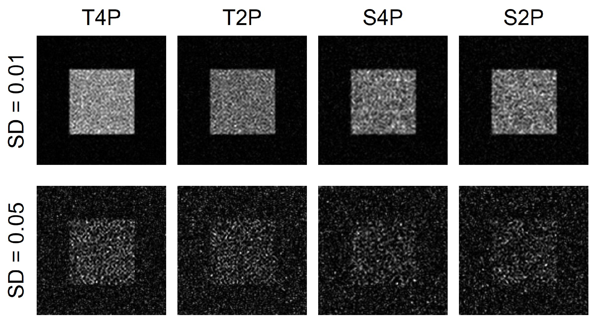
| T4P | T2P | S4P | S2P | |
|---|---|---|---|---|
| CV: SD | 0.194 | 0.265 | 0.288 | 0.289 |
| CV: SD | 0.722 | 0.830 | 0.839 | 0.869 |
Disclaimer/Publisher’s Note: The statements, opinions and data contained in all publications are solely those of the individual author(s) and contributor(s) and not of MDPI and/or the editor(s). MDPI and/or the editor(s) disclaim responsibility for any injury to people or property resulting from any ideas, methods, instructions or products referred to in the content. |
© 2024 by the authors. Licensee MDPI, Basel, Switzerland. This article is an open access article distributed under the terms and conditions of the Creative Commons Attribution (CC BY) license (https://creativecommons.org/licenses/by/4.0/).
Share and Cite
Yoneda, N.; Liu, J.-P.; Matoba, O.; Saita, Y.; Nomura, T. Computational Optical Scanning Holography. Photonics 2024, 11, 347. https://doi.org/10.3390/photonics11040347
Yoneda N, Liu J-P, Matoba O, Saita Y, Nomura T. Computational Optical Scanning Holography. Photonics. 2024; 11(4):347. https://doi.org/10.3390/photonics11040347
Chicago/Turabian StyleYoneda, Naru, Jung-Ping Liu, Osamu Matoba, Yusuke Saita, and Takanori Nomura. 2024. "Computational Optical Scanning Holography" Photonics 11, no. 4: 347. https://doi.org/10.3390/photonics11040347
APA StyleYoneda, N., Liu, J.-P., Matoba, O., Saita, Y., & Nomura, T. (2024). Computational Optical Scanning Holography. Photonics, 11(4), 347. https://doi.org/10.3390/photonics11040347