1. Introduction
Adaptive Optics (AO) is a technology that makes real-time corrections to distorted wavefronts by dynamically adjusting the control signal of a corrector based on wavefront sensing data, which was first proposed by American astronomer H.W. Babcock in 1953 [
1]. Over the past 60 years, AO has significantly developed and is now widely used in various fields such as astronomy [
2], Free space optics [
3], and microscopy [
4]. As optical systems become more complex and find applications in more extreme scenarios, the wavefront disturbance caused by atmospheric turbulence often exhibits higher temporal variability, which places greater demands on AO systems’ wavefront sensing and processing performance [
5,
6].
In recent years, researchers have been working to enhance AO systems’ performance by improving wavefront sensing and processing speed, which has been mainly achieved by applying electronic neural networks to data processing and system control [
7,
8,
9,
10]. Although these methods have reduced time consumption to some extent, they still require a large amount of data conversion and complex calculations due to the limitations of electronic computation. In contrast, recent architectures based on optical computation have shown considerable promise, particularly in object classification [
11] and saliency detection [
12] applications. Compared to electronic methods, these optical approaches demonstrate unparalleled speed advantages and comparable sensing accuracy.
Considering the wavefront sensing and processing task receiving optical signals as inputs, optical computation emerges as a promising avenue for acceleration. Significant progress has been made in this area. Pan et al. proposed a diffractive adaptive optics system (DAOS) architecture. This wavefront sensor-less AO system can achieve wavefront correction for converging light beams entirely through optical means, thereby enhancing the imaging quality of point targets [
13]. Zhan et al. also employed an optical neural network to correct wavefront distortion generated by oceanic turbulence in an underwater wireless optical communication (UWOC) system [
14]. Furthermore, Goi et al. introduced an Integrated Diffractive Deep Neural Networks (ID
2N
2) method [
15]. This hybrid photonic-electronic integrated deep neural network directly reconstructs the optical pupil phase as an intensity distribution through optical computation.
Although the methods mentioned above have provided insights into the application of optical computation in wavefront sensing and processing, there are still challenges in working with other components of the AO system. For instance, these methods exhibit sensitivity to overall or local perturbations in intensity distribution, thereby limiting their generalization capabilities, especially in harsh atmospheric conditions. Moreover, the coupling between these methods and the following wavefront correctors still necessitates extensive post-processing of data, which, due to the “weakest link” effect, continues to constrain the overall operational bandwidth of the AO system.
In this paper, we propose an integrated wavefront sensing and processing (IWFSP) method, which employs a diffractive optical neural network to replace traditional wavefront sensors and processors, specifically optimized for seamless integration with subsequent wavefront correctors to form a high-bandwidth AO system. In the simulation section, we generate a dataset of wavefront aberrations and train the diffractive neural network to perform wavefront sensing and processing tasks, followed by a numerical analysis of its performance. In the experimental section, we demonstrate wavefront correction based on IWFSP through benchtop experiments, preliminarily validating the feasibility of this method for constructing AO systems. In the discussion section, we propose several potential hardware improvement measures and further analyze the bandwidth of adaptive optical systems based on this approach.
2. Simulation
The IWFSP proposed in this paper is essentially an optical neural network optimized for wavefront sensing and processing tasks, which is a variant of the diffractive deep neural network (D
2NN). Introduced by Lin et al. from the University of California, D
2NN is an optical computation architecture based on the diffraction effect, enabling specific inference tasks at the speed of light [
11]. The implementation process of IWFSP, like a typical D
2NN, comprises two stages: electronic training and optical deployment. The electronic training stage can be seen as an automatic design process for the modulation layer of the optical field on an electronic computing platform. It is data-driven, utilizing abundant sample data to update parameters through deep learning algorithms iteratively. A comparison between the D
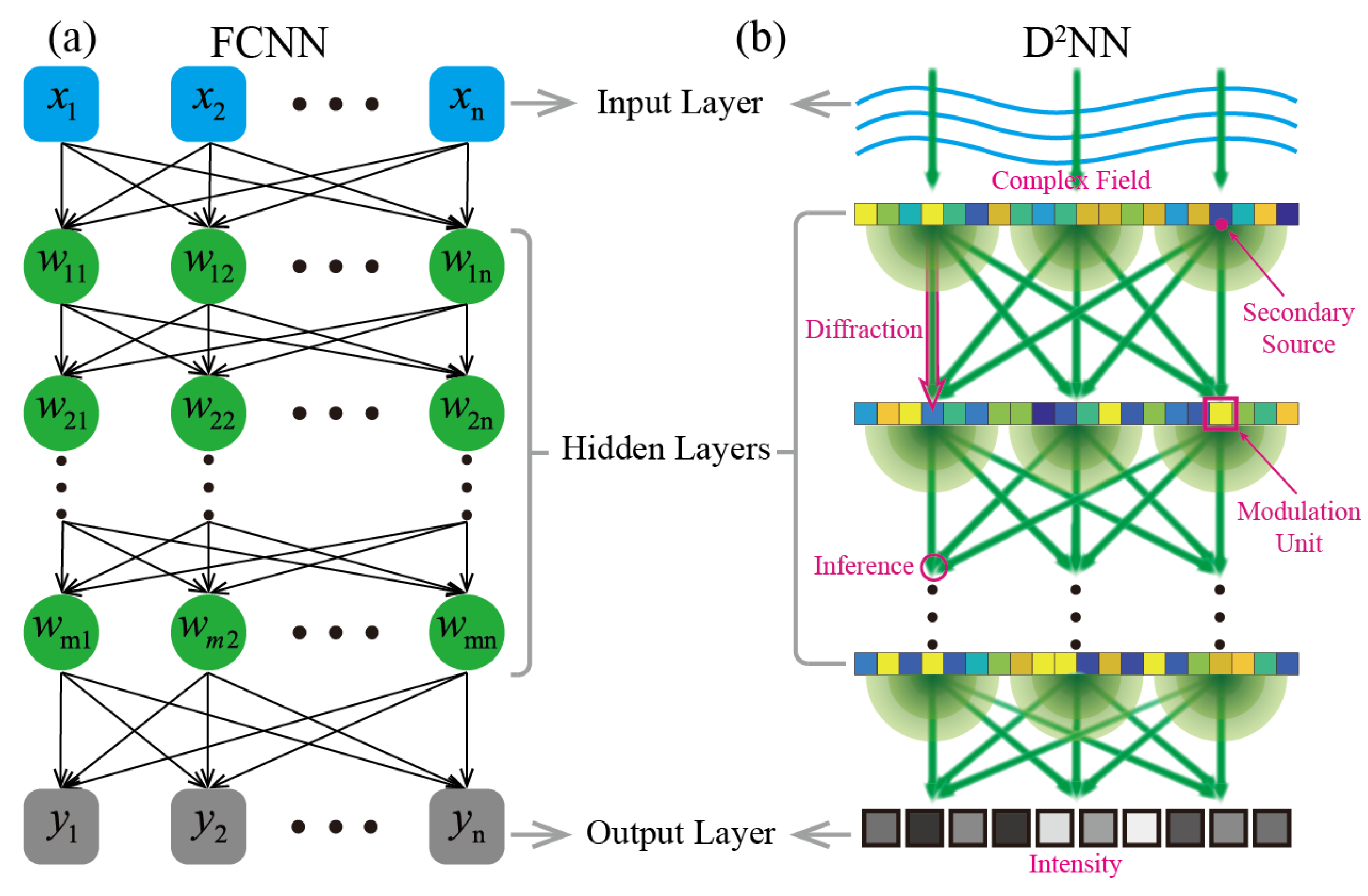
2NN and the classical Fully Connected Neural Network (FCNN) is illustrated in
Figure 1, where both consist of input, hidden, and output layers. Unlike electronic neural networks, in D
2NN, the interconnection between neurons is described by optical diffraction theory, which implies that the forward propagation of this model can be regarded as a numerical simulation of spatial light modulation and diffraction for a specific complex field. Consequently, based on the free-space optical interconnection, the parameters of the neural network trained electronically correspond to the modulation coefficients of spatial light, which can be deployed to achieve optical computation for specific tasks.
According to the description of the angular spectrum method, the diffraction propagation phenomenon of light can be regarded as a linear spatial filter, assuming that the complex field at
is
, then the complex field at
z position is
where the transfer function
is
therefore, based on the Huygens–Fresnel principle, the interconnection formula between neurons in adjacent layers of the neural network can be obtained as
where
represents the input of the neuron labeled
k in the next layer, and
represents the output of the neuron labeled
i in the previous layer.
Considering that the classical D
2NN architecture is only capable of handling classification problems based on the maximum output intensity, we introduce an improvement by incorporating differential operations to extend its inference capability to regression problems [
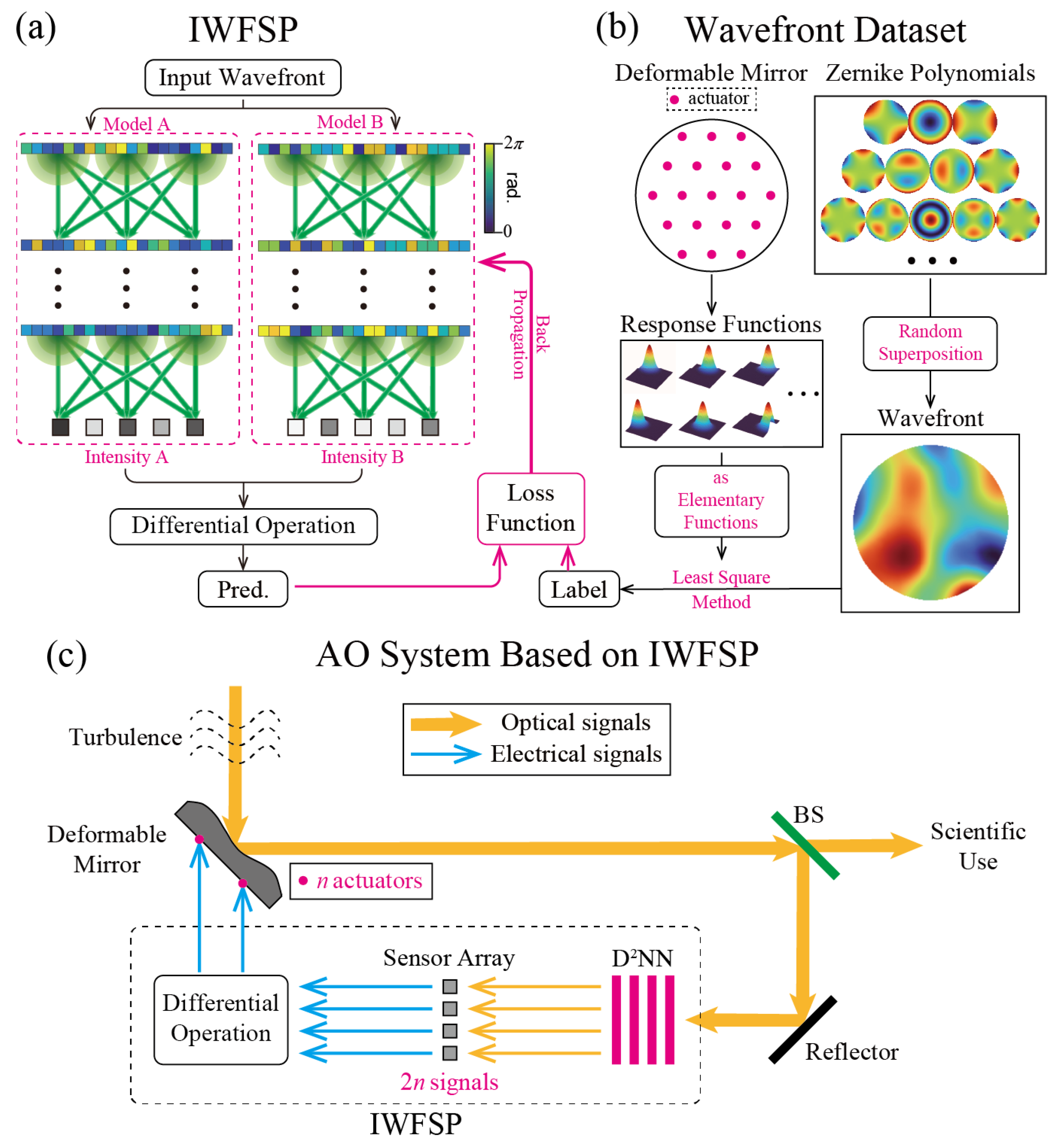
16]. The improvement method involves integrating a pair of parallel D2NNs through differential operations into the same model for synchronous optimization, as illustrated in
Figure 2a. This enhancement not only alleviates the strict non-negativity constraints on output light intensity but also enhances the robustness of the model to both overall and local perturbations in input light intensity, thereby contributing to the improvement of the model’s accuracy.
Additionally, we have specifically optimized the IWFSP for subsequent collaboration with the deformable mirrors, where output intensity signals, after simple differential operations, can be directly utilized to control actuators for correction, thereby constructing a high-bandwidth AO system, as illustrated in
Figure 2c. When working, a wavefront sensor in a traditional AO system, such as the Shack–Hartmann wavefront sensor (SH-WFS), first needs to collect the intensity distribution at the focal plane of the microlens array, and then calculate the intensity center of mass within the sub-aperture, and then The local slope of the wavefront is calculated based on the offset of the center of mass from the ideal focus, and finally the wavefront is reconstructed based on the slope of the wavefront. Then, the wavefront processor computes actuator control signals based on the reconstructed wavefront and the optical response function of the deformable mirror, involving extensive and complex matrix operations. Then, the wavefront processor needs to calculate the control signals of actuators based on the reconstructed wavefront and the optical response function of the deformable mirror, which involves a large number of complex matrix operations. In contrast, the proposed IWFSP method accomplishes most of the computations during wavefront sensing and processing using optical neural networks, resulting in minimal data volume for subsequent electronic operations. For a deformable mirror with
n actuators, only
intensity signals need to be detected and subjected to simple differential operations, significantly reducing the time required for wavefront sensing and computation processes.
Firstly, in order to train the diffractive optical neural network for wavefront sensing and processing tasks, we compiled a dataset of wavefronts. We generated 10,000 wavefront distortion samples using Zernike polynomials with random coefficients, as shown in
Figure 2b. Zernike polynomials, introduced by Zernike in 1934 [
17], constitute a complete orthogonal basic function set on the unit circle, making them suitable for fitting aberrations on circular pupils. These wavefront samples are generated using Zernike polynomials up to the 28th order (according to Noll indices), with random coefficients following Gaussian distributions of varying standard deviation. The coefficients of Zernike polynomials of all samples can be found in the
Supplementary Materials. These samples were employed for the electronic training process, with 6,000 randomly selected for training, 2000 for validation, and 2000 for testing. As part of integrating wavefront processing capabilities, we used the optical response functions of a 19-actuator deformable mirror as elementary functions. Each sample’s label represents the decomposition coefficients of the wavefront on this set of elementary functions. Expanding each response function into a vector and concatenating them into a response matrix,
R. For a random wavefront distortion sample
X, its label
L is given by the least-squares solution to the equation
.
During the electronic training process, we constructed an IWFSP model using Python 3.10.11 and PyTorch 2.0.1 frameworks, with specific parameter configurations shown in
Table 1. We set the physical size of a single neuron to
μm, determined by the pixel size of the SLM used in the subsequent experiment. Additionally, the input wavelength was set to 532 nm, determined by the laser source used in the experiment. After determining the neuron size and input wavelength, it was necessary to choose an appropriate inter-layer distance to ensure full connectivity of the neural network. Considering a single diffraction modulation layer as a grating with modulation unit physical size
d and incident light wavelength
, under normal incidence conditions, the diffraction angle
satisfies the following equation according to the grating equation
where
m represents the diffraction order, where the primary diffraction peak corresponds to
. As
m increases, the intensity of the diffraction peaks gradually decreases. Therefore, we choose
to determine the maximum diffraction angle, as follows:
For the
nm and
μm used in this simulation, the maximum diffraction angle is calculated to be
. Considering that each layer of the neural network contains
neurons, in order to achieve full connectivity, the inter-layer spacing
l must satisfy
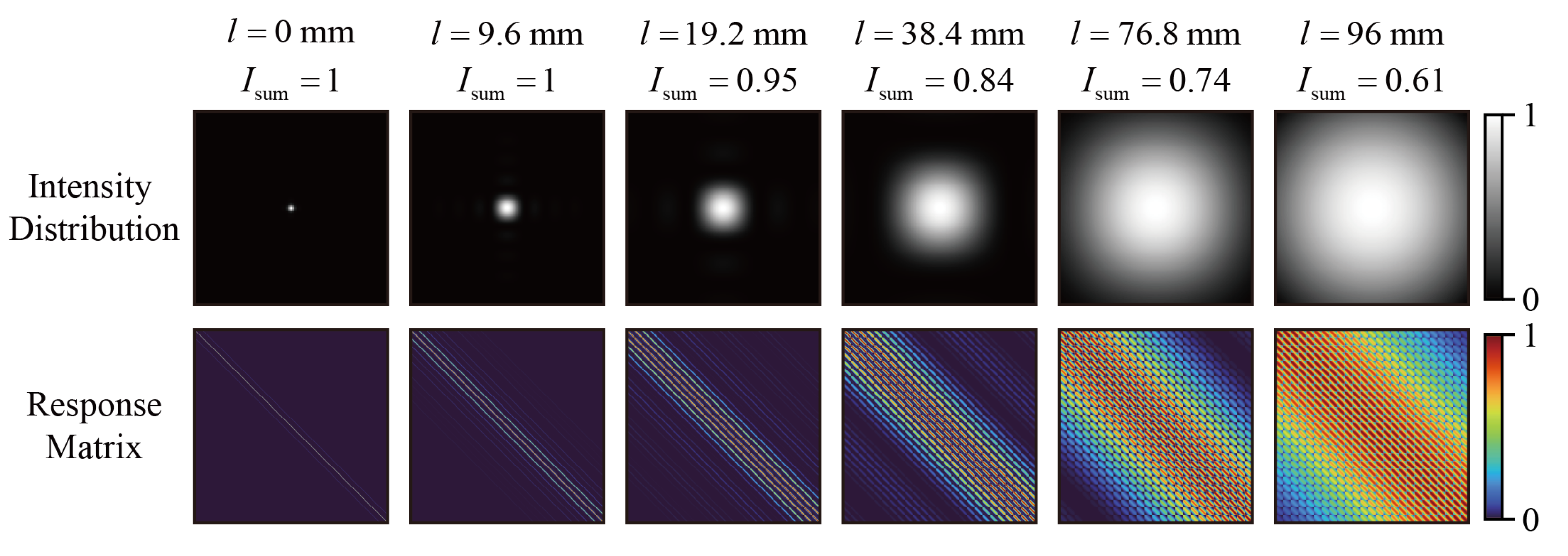
Furthermore, we validated this through numerical simulations of the diffractive response matrix at different distances. As mentioned earlier, the diffraction propagation phenomenon of light can be regarded as a linear system. For a diffractive layer containing
neurons, it has
inputs and
outputs. By applying unit excitation to each neuron and observing output intensities at different distances, we obtained multiple diffractive response matrices of size
, as depicted in
Figure 3. It is important to note that both the intensity distribution and the response matrices in the figure have been normalized. It can be observed that with increasing distance, the response of edge neurons becomes more pronounced. However, the total intensity decreases because some of the light propagates outside the calculation window. This implies the necessity of selecting an appropriate inter-layer spacing
l to maintain a high utilization of light intensity while satisfying the fully connected characteristic of the diffraction neural network. Consequently, in this study, we chose an inter-layer spacing of
cm.
Besides the four diffractive layers, the construction of the IWFSP model also incorporates a front-end input layer and an end-stage differential layer. The input layer loads wavefront data from the dataset onto the phase channel of the beam. The differential layer integrates the output intensities of the two parallel models, providing final differential predictions to enable joint training. The forward propagation of this neural network model is implemented using angular spectrum method, and the loss function is represented by the mean squared error (MSE) between the differential predictions and the labels of the samples. Error back-propagation is performed using the adaptive moment estimation (Adam) algorithm. For the Adam optimizer, the initial learning rate is set to , with coefficients for computing the running averages of gradients and their squares set as and , respectively. To improve numerical stability, is added in the denominator. Additionally, we apply the sigmoid function to the parameters of the neural network to confine the phase modulation coefficients within the range .
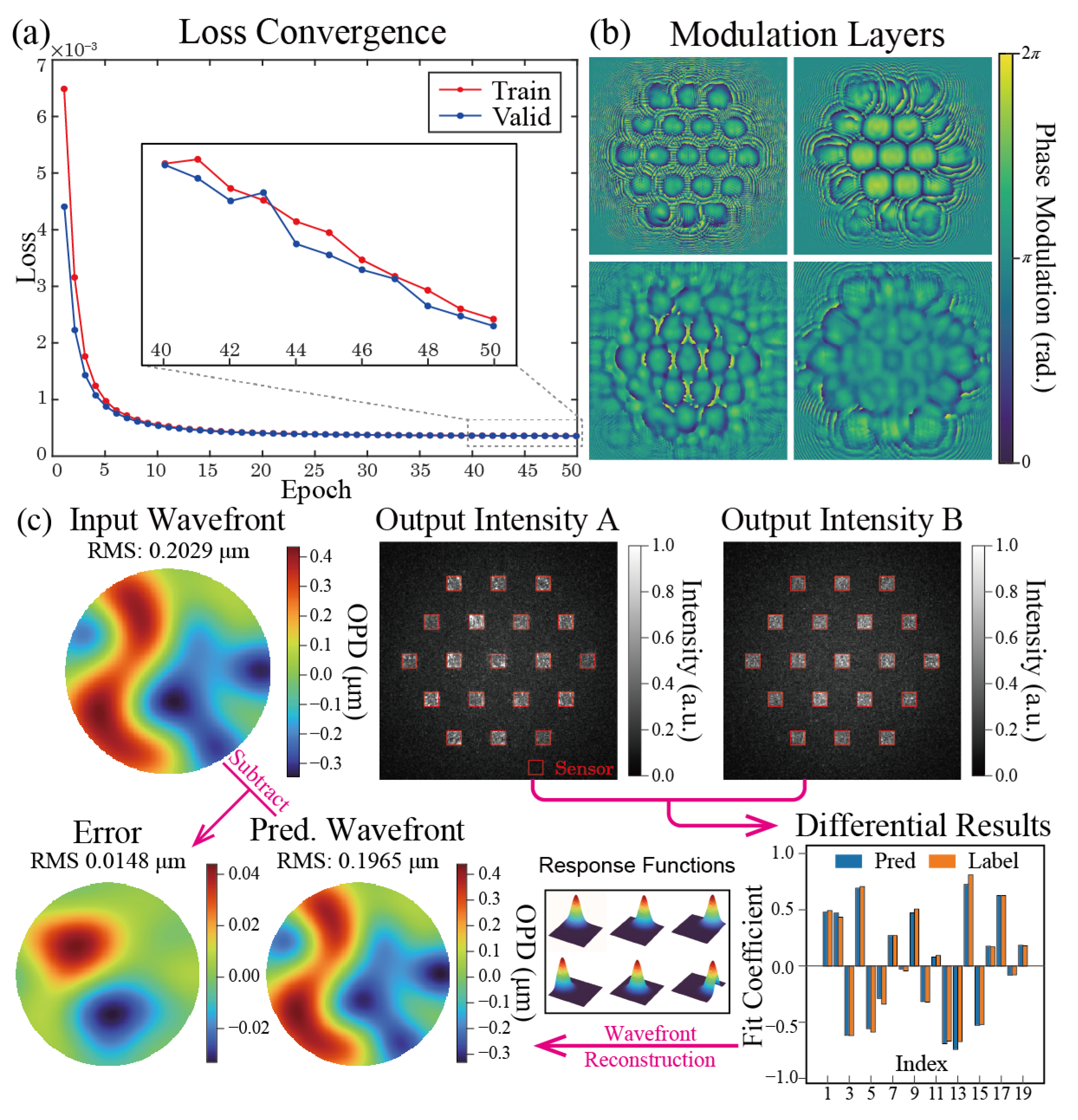
As depicted in
Figure 4a, after 50 epochs of training, the IWFSP model exhibits a convergence of the loss function, reaching its minimum on both the training and validation datasets, Which indicates optimal performance and generalization capability. Further training might offer marginal performance improvements but could potentially lead to overfitting. Therefore, we performed a detailed performance analysis for the 50-epoch model.
Parameters of the trained IWFSP model are extracted and transformed to obtain the final optimized design for the cascaded phase modulation layers, as shown in
Figure 4b. After training with a large dataset, the model forms specific modulations at positions corresponding to the peak values of the response functions, establishing a connection between the input wavefront’s local information and the target region’s light intensity. From the wavefront sensing and reconstruction process of a random sample in
Figure 4c, it is evident that after optical computing through phase modulation layers, the model provides two sets of discrete light intensity distributions on the output plane. Assuming subsequent collaboration of IWFSP with a deformable mirror containing
n actuators, models A and B will, respectively, output
n discrete output light intensities, denoted as
and
. The final prediction value
of IWFSP is determined by the following differential operation:
where
K is a scalar hyperparameter of the model, used to amplify the results of differential operations, thereby allowing smaller differences in light intensity to produce larger output signals. In both the simulations and experiments of this study, the value of K was set to 4. The value was determined as the optimal result by training multiple models while keeping other model and training hyperparameters unchanged. We varied this hyperparameter between 1 and 5 at intervals of 1 and conducted hyperparameter evaluations on the validation set, ultimately yielding the optimal result of 4. Additionally, due to the generation of the optical response function for a 19-actuator deformable mirror in this simulation (i.e., n = 19), models A and B output 19 intensity signals each, totaling 38 data points. This data volume is significantly smaller than what is required by traditional wavefront sensors and processors. It is worth noting that the 19 values of the differential prediction result
correspond to the control signals of the 19 actuators of the deformable mirror, which, after simple voltage amplification, can be directly used to guide the deformable mirror in correcting wavefront distortions.
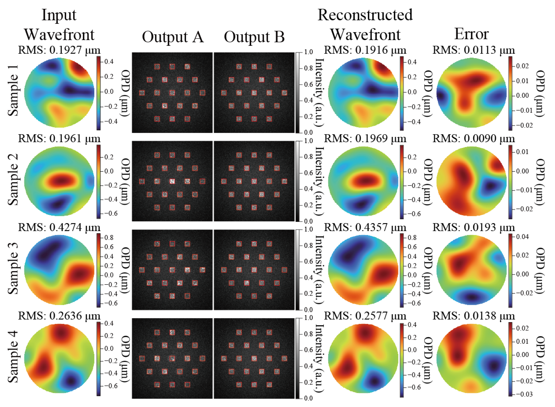
After obtaining the predicted values, we can multiply them with the corresponding elementary function and then superimpose sum them up to obtain the final reconstructed wavefront. The wavefront sensing results of four random test data not used during the training process are shown in
Figure 5, indicating its ability to generalize to a certain extent. We then conducted traversal verification on the test set of 2000 samples and calculated that the input wavefront’s average Root Mean Square (RMS) value was 0.2849 μm. The average RMS of sensing error was 0.0167 μm, which accounts for only 5.86% of the input wavefront RMS. Therefore, it can be concluded that IWFSP has high-precision sensing performance, which is comparable to traditional wavefront detection methods.
3. Experiment
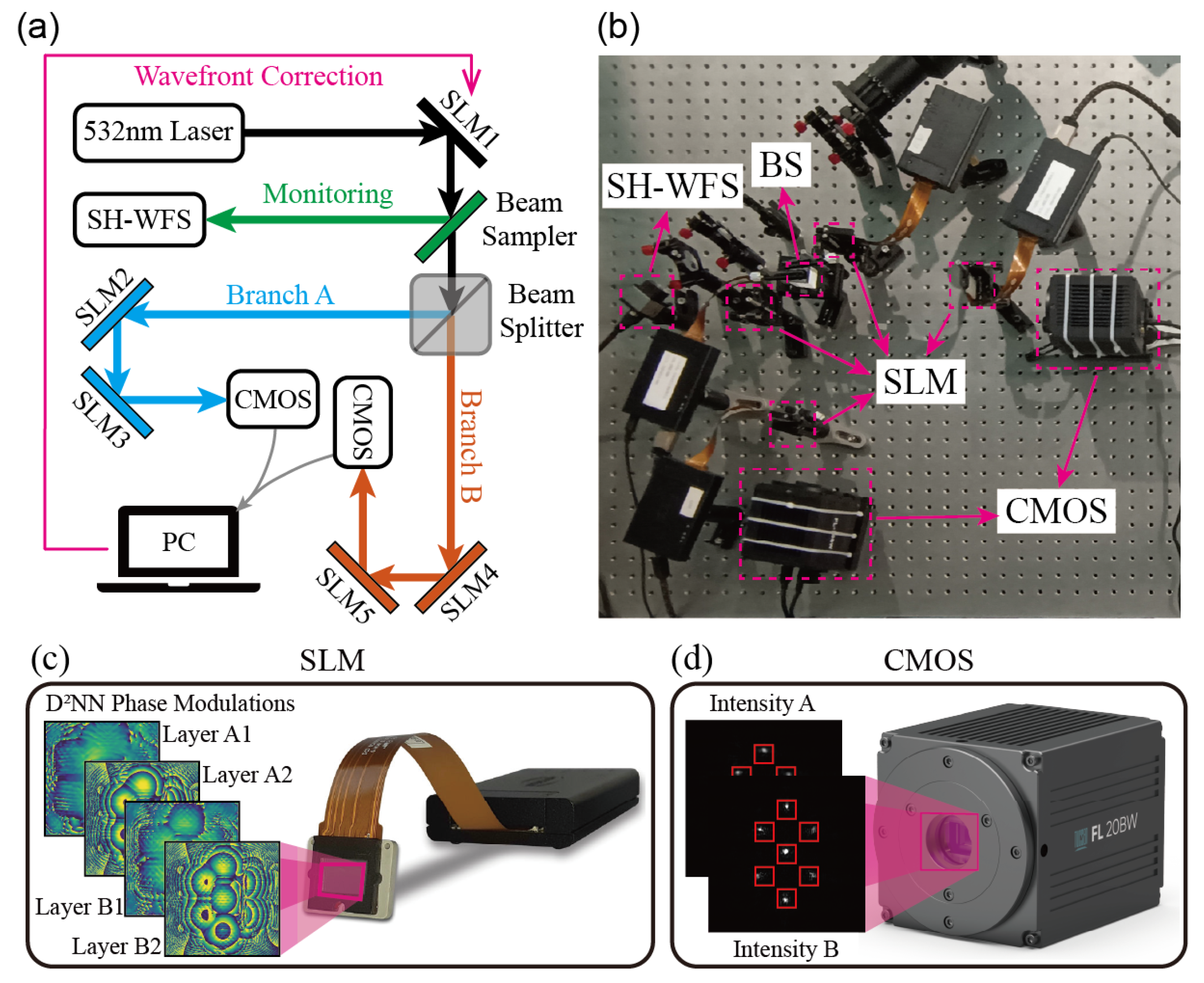
Following numerical simulations, we conducted benchtop experiments to validate the feasibility of the IWFSP method for wavefront correction, as illustrated in
Figure 6. In this experiment, we employed a continuous-wave laser with a wavelength of 532 nm as the illumination source, generating a circular beam with an approximate diameter of 5 mm. Following the laser, we placed a Spatial Light Modulator (SLM) to introduce wavefront aberrations into the beam. The SLM, an electro-optic modulating device, alters the arrangement of liquid crystal molecules by applying varying electric fields, thereby modifying the refractive index of the liquid crystal layer to modulate the incident wave. Specifically, we utilized reflective phase-type SLMs, which receives 8-bit grayscale image data as input and adjusts the phase of corresponding elements based on the grayscale values of the image pixels, where a grayscale value of 255 corresponds to a phase modulation of 2
. In the experiment, we randomly selected wavefront samples from the test dataset, converted them into grayscale images, and loaded them onto the first SLM to introduce wavefront aberrations. Subsequently, we constructed a monitoring branch using a beam sampler to quantitatively measure the wavefront of the beam using a Shack-Hartmann Wavefront Sensor (SH-WFS). Then, we split the beam into two branches, A and B, using a 1:1 beam splitter (BS), each equipped with two SLMs to deploy phase modulation layers designed by IWFSP corresponding to Model A and Model B. Finally, a Complementary Metal Oxide Semiconductor (CMOS) camera was placed at the end of each branch to capture the output intensity.
In this experiment, considering inter-layer misalignment of the neural network, we retrained a new model with neurons for each layer using only the central 7 actuators of the 19-actuator deformable mirror employed in simulations. This adjustment was made to reserve 280 pixels of the SLM for alignment correction. Apart from the number of actuators and neurons, all other parameters of this model remained identical to those used in the simulations. Inter-layer alignment error is one of the primary factors affecting the deployment performance of D2NN. Therefore, to address the alignment issues inherent in deploying D2NN based on SLMs, this study employs a holographic imaging-based alignment method. By loading a holographic modulation image onto the first SLM, a cross-shaped pattern is formed on the surface of the second SLM. If there is any deviation between the center of this cross and the center of the second layer SLM, calibration can be achieved by shifting the phase modulation pattern on the first layer. Considering the pixel size of the SLM is 8 μm, this method theoretically enables alignment accuracy up to 8 μm.
Subsequently, we extracted the trained D
2NN model parameters, transformed them into phase modulations using the sigmoid function, and loaded them to the corresponding SLM. Considering that there are some inevitable deployment errors in the optical implementation of IWFSP, we have made some corrections to the differential operation. If the two output light intensities corresponding to the
m-th actuator of the deformable mirror are denoted as
and
, then the actuator’s control signal is given by the following equation
where
is employed to correct the background noise of the CMOS and the incompletely shielded ambient light.
is utilized to correct the uneven beam splitter ratio. Both parameters can be determined through a calibration process before the experiment. After adjusting the optical path and completing the alignment process, without turning on the laser source, the intensity of light is collected using the two CMOS sensors at the end, which can be utilized to calibrate the
parameters for each target area. Subsequently, with the light source turned on, the intensity of light is once again captured using the two CMOS sensors at the end. The collected intensities are subtracted by
to eliminate background noise. Finally, the output intensity of branch A is divided by the output intensity of branch B to obtain the calibrated parameter value
.
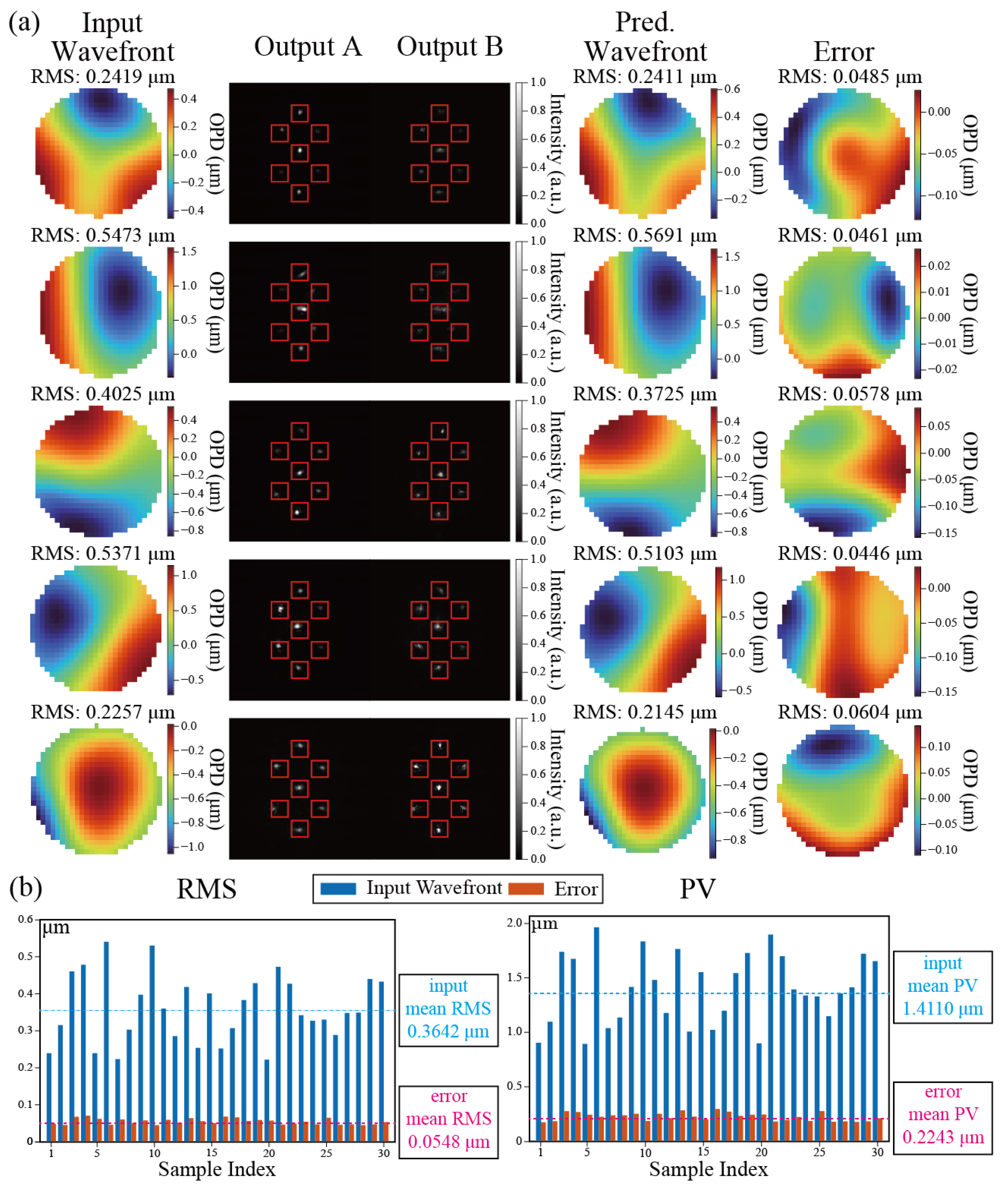
After setting up the experimental platform and completing the necessary calibration procedures, we conducted tests on 30 randomly generated wavefront distortion samples. The experimental results for five random samples are shown in
Figure 7a. The reconstructed wavefront from IWFSP is combined after taking the negative and superimposed onto the input wavefront, allowing SH-WFS to detect the correction residuals. This process serves as a simplified simulation of the actual workflow of an AO system.
Figure 7b displays the Peak-to-Valley (PV) and RMS values before and after correction for all 30 wavefront distortion samples tested in the experiment. The average RMS of the input wavefront distortions is 0.3642 μm, with an average PV of 1.4110 μm. After correction by IWFSP, the average RMS of the residual wavefront is reduced to 0.0548 μm, with an average PV of 0.2243 μm, indicating an error of approximately 15%.
The above experimental results further confirm the capability of the IWFSP method to perform sensing and processing of the input wavefront through optical computation, directly solving the control signals based on the corrector of the AO system. A particular discrepancy between the experimental and simulated results could be attributed to the deployment errors, which can be addressed by introducing an in-situ training method [
18] or vaccination strategy [
19].
4. Discussion
Through the above simulation and experiment, we have proven that IWFSP can optically realize most of the operations in wavefront sensing and processing. Compared with traditional wavefront sensing and processing methods, the IWFSP method can be seen as shifting the majority of computations before sensing, effectively achieving “optical-domain data preprocessing”, which will significantly enhance computational speed and reduce data volume. It is worth noting that there are no restrictions on the elementary functions used for wavefront reconstruction in IWFSP. In this study, the optical response function of the deformable mirror is used as the elementary function. The advantage is that it can realize the direct optical solution of the control signal of the deformable mirror. Furthermore, this approach offers the flexibility to utilize Zernike polynomials as basis functions. In this scenario, the method can function as a rapid wavefront sensor, providing direct estimation of the fitting coefficients for various orders of Zernike polynomials characterizing the input wavefront.
In the verification experiment of this study, CMOS cameras were utilized to capture the distribution of light intensity. This decision was made for experimental convenience and to facilitate result analysis and performance evaluation. Actually, the final control signal predicted by IWFSP does not need to be obtained from the high-resolution light intensity distribution. Rather, it only requires the total intensity data of light within small regions on the output plane, which is the advantage of “optical-domain data preprocessing”. This means that in actual applications, only photodiodes can be used to detect intensity signals (n is the number of actuating units of the deformable mirror). This not only improves the sensing speed, but also completes the summation of light intensity in the target area through the sensing method of the photodiode device itself, further reducing the amount of calculations. In addition, SLMs were adopted for the optical deployment of IWFSP in the experiment. In practice, diffractive neural networks can be deployed through micro/nanostructures to reduce volume and mass and achieve compact small detectors. Considering experimental convenience, a computer was employed for conducting differential operations. In fact, differential calculations involve only basic arithmetic operations such as addition, subtraction, multiplication, and division, which can be efficiently implemented by Field-Programmable Gate Array (FPGA) circuits. This approach would enhance processing speed further through parallel computing optimization.
Most of the IWFSP data is processed using parallel optical computing, so its processing time is equivalent to the time required for light to travel. For our simulation and benchtop experiment examples presented in this article, the optical path distance from the wavefront input surface (SLM1) to the intensity output surface (CMOS) is less than 1 m. If the miniaturized deployment solution mentioned above is adopted, the distance can be further reduced to within 0.1 m. Therefore, the time consumption of the optical calculation part is on the order of nanoseconds and can be ignored. The subsequent differential operation also requires much less data compared to traditional methods. For the 19-actuator deformable mirror, only 38 intensity data need to be calculated. Even if multiple calibration coefficients are taken into account, the amount of data required to be processed does not exceed one hundred, which is far smaller than the tens of thousands of image pixel data in traditional methods. More importantly, IWFSP can compress wavefront data into several intensity characteristics, significantly reducing the time required for processes such as photoelectric conversion and analog-to-digital conversion. Generally speaking, the rise time of conventional photodiodes is usually on the order of hundreds of nanoseconds to microseconds, and even considering analog-to-digital conversion, it only takes tens of microseconds. If the subsequent differential operation of hundreds of data is implemented by FPGA, it may take a time ranging from a few microseconds to dozens of microseconds. If parallel computing optimization is fully considered, higher levels can be achieved. Therefore, compared with traditional methods, the frame time based on IWFSP is approximately within a hundred microseconds and can reach an operating bandwidth of at least 10 kHz. If it is subsequently used in combination with a high-speed deformable mirror to form an AO system, considering the iterative correction of about 10 frames, its closed-loop bandwidth can also reach the kHz level. This is much higher than the closed-loop bandwidth of tens to hundreds of Hz of existing classic AO systems.
In addition, with the growing demand in astronomical observations and other fields, the scale of AO systems is also increasing. Extreme AO systems often contain wavefront sensors with thousands of sub-apertures and wavefront correctors with thousands of actuators, which will dramatically increase the amount of data and time-consuming wavefront processing [
5]. AO systems based on traditional wavefront sensing and processing methods will inevitably face bottlenecks in scale and bandwidth in the future. The AO system based on IWFSP introduces optical operations to achieve parallel processing, which greatly compresses the amount of data and can maintain a high processing speed even in extreme AO systems. Therefore, the IWFSP method is expected to resolve the conflict between the scale and bandwidth of future AO systems.


