Abstract
Monocular stereo vision has excellent application prospects in the field of microrobots. On the basis of the geometric model of bifocal imaging, this paper proposes a monocular depth perception method by liquid zoom imaging. Firstly, the configuration of a monocular liquid vision system for depth measurement is presented, and the working mechanism of the system is analyzed through theoretical derivation. Then, to eliminate the influence of optical axis drift induced by the liquid gravity factor on the measurement results, the target image area is used as the calculation feature instead of the image vector length. A target area calculation method based on chain code classification and strip segmentation is proposed. Furthermore, in response to the fluctuation problem of liquid lens focal power caused by factors such as temperature and object distance, a dynamic focal length model of the liquid zoom imaging system is constructed after precise calibration of the focal power function. Finally, a testing experiment is designed to validate the proposed method. The experimental results show that the average error of depth perception methods is 4.30%, and its measurement time is only on the millisecond scale. Meanwhile, the proposed method has good generalization performance.
1. Introduction
Microrobots, due to their small size, good concealment, and strong mobility, can achieve functions such as target localization and autonomous obstacle avoidance by equipping them with corresponding optical payloads [1]. It has important applications in military reconnaissance, hazardous material disposal, and equipment support. Among them, the ability of three-dimensional visual measurement is a key factor affecting the task capacity of robots. The traditional stereo vision scheme is to obtain stereo image pairs by shooting the same object with two or more cameras. Then, parallax is calculated by the image-matching algorithm, and the target depth information is obtained by combining the principle of triangulation [2]. Compared with binocular/multi-vision, depth measurement technology based on monocular imaging has advantages in micromachine vision applications due to its smaller hardware size, and further research is needed.
The depth measurement methods by monocular vision are mainly divided into three categories: focusing method [3], defocus method [4], and zoom method [5]. The zoom method achieves stereo imaging by changing the focal length of the imaging system and then obtaining the distance information of the target based on image processing technology. Ma et al. [6] first proposed the depth estimation method by zoom lens and discussed the zoom image processing scheme based on gradient and feature. The research theoretically indicates that zoom images can provide target depth information. Baba et al. [7] established a zoom lens model based on the solid lens structure, which includes zoom, focus, and aperture parameters. On this basis, a depth measurement method based on the edge blur changes of the image was proposed, and its applicability was evaluated. Xu et al. [8] theoretically analyzed the monocular bifocal stereo imaging model. He proposed corresponding feature detection and matching methods and combined them with camera calibration results to achieve monocular 3D reconstruction of the scene. Huang et al. [9] applied zoom imaging ranging to three-dimensional localization of cell particles.
From the current research status, monocular vision measurement based on zoom image adopts an all-solid displacement zoom system; that is, the zoom and focusing functions are achieved by driving multiple solid lenses with relative displacement through a motor. Due to the limited response speed of displacement optical zoom systems, fast zoom imaging cannot be achieved, which will affect the real-time performance of monocular vision measurement. A liquid lens is a new type of optical element developed based on the concept of bionics that can achieve autonomous focal length adjustment by changing the contour of the liquid interface. When applied to the design of an optical zoom system, the system has significant advantages in response speed and structure dimension compared with an all-solid lens [10]. In this regard, this paper intends to combine liquid photon technology with visual measurement theory to carry out innovative research. On the basis of providing the configuration of a monocular liquid vision system, a monocular depth perception method based on liquid zoom imaging is established, and the effectiveness of the method is tested and analyzed through experiments.
2. Principles and Methods
2.1. System Components
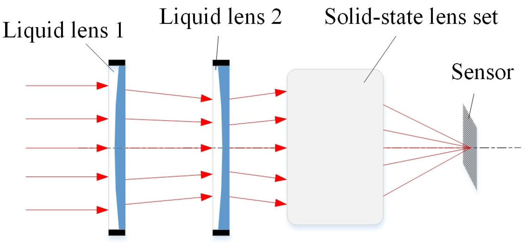
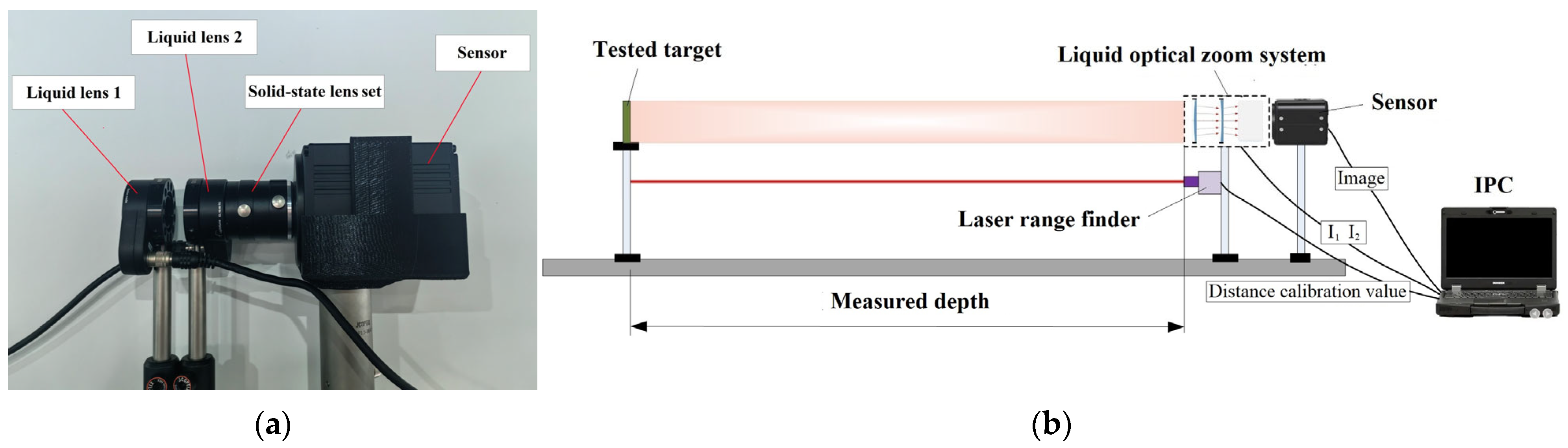
The designed monocular vision system consists of two liquid lenses, a solid-state lens set, and a sensor, as shown in Figure 1. Among them, liquid lens 1 is mainly adopted to compensate for image plane offset, which is equivalent to the compensation unit. Liquid lens 2 is mainly adopted to change the focal length of the system, which is equivalent to the variable magnification unit. The solid-state lens set plays a role in maintaining focal power and correcting aberrations.
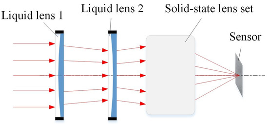
Figure 1.
The configuration of monocular liquid vision system for depth measurement.
The host computer sends the serial command to the liquid lens and controls the input current of liquid lens 1 and liquid lens 2 in real time through the special drive circuit board. The Gaussian bracket method [11] is adopted to describe the total focal power and image stability conditions of a liquid monocular vision system. It can be deduced that the focal power of each component in the zoom process satisfies the following relationship:
where Φ is the total focal power of the optical system; φ1 is the focal power of liquid lens 1; φ2 is the focal power of liquid lens 2; φ3 is the focal power of the solid lens group; d1 is the distance between liquid lens 1 and liquid lens 2; d2 is the distance between liquid lens 2 and solid lens group; and d3 is the distance between the solid-state lens set and the sensor.
The value of φ1 varies with the input current I1. The value of φ2 varies with the input current I2. Under the condition that φ3, d1, d2, and d3 are set to a fixed value (no moving components), the liquid zoom imaging module can continuously and rapidly adjust the total focal length (total focal power) of the system and maintain clear imaging by controlling the input current I1 and I2. The zoom and autofocus process has no moving components. Due to the extremely fast response speed of liquid lenses, the liquid vision system shown in Figure 1 can achieve rapid switching between wide and narrow fields of view.
2.2. Depth Measurement Method
2.2.1. Theoretical Basis
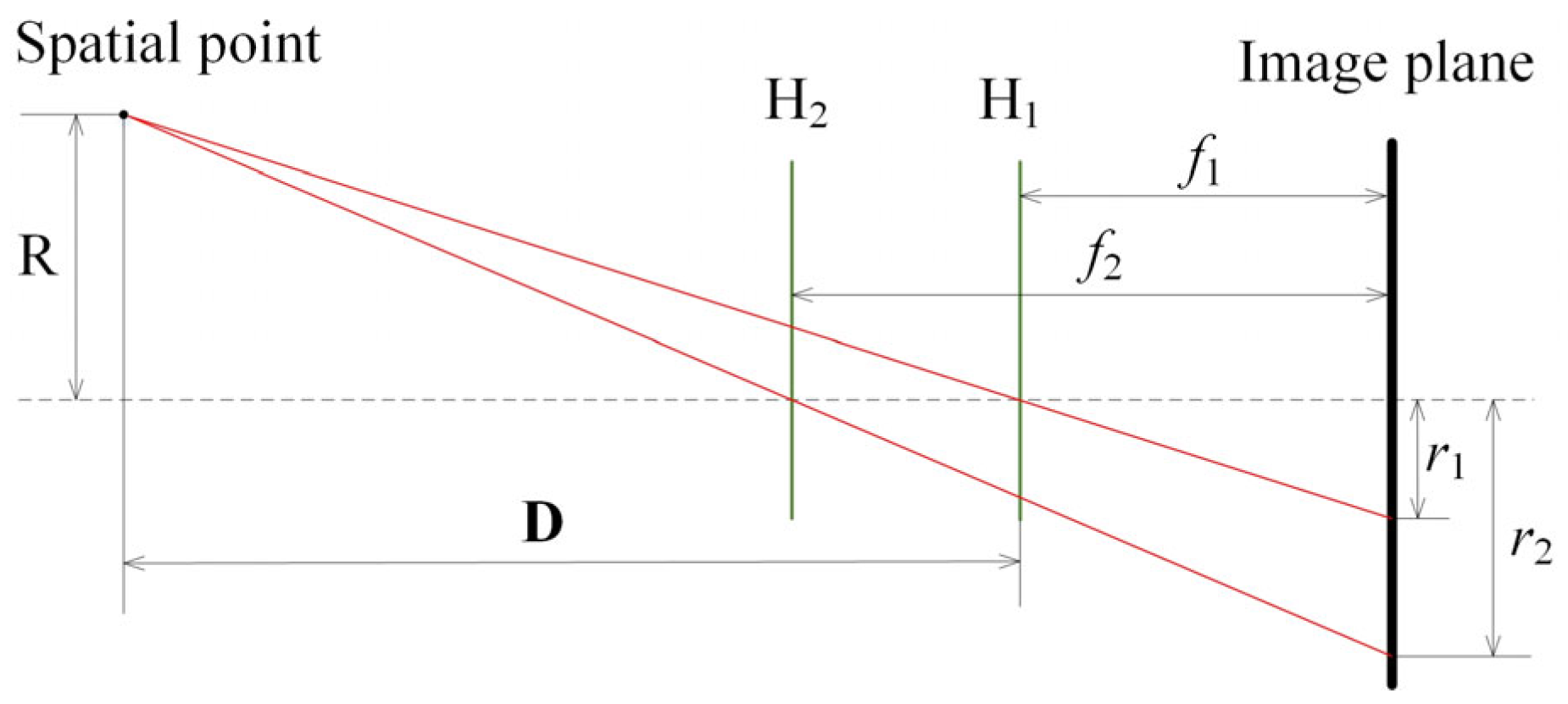
According to geometric optics, there is a quantitative relationship between the depth of spatial objects and the image vector length, as well as the corresponding focal length. Therefore, by searching for matching point pairs in two zoom images, the image vector length can be obtained. On the basis of solving the corresponding focal length, the depth information of the spatial objects can be calculated. By simplifying the monocular vision system into a pinhole model, the imaging geometric models of the system in small focal length f1 and large focal length f2 states can be obtained, as shown in Figure 2.
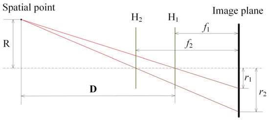
Figure 2.
Geometric model of monocular zoom imaging.
H1 and H2 represent the principal planes of the image in small focal length (wide field of view) and large focal length (narrow field of view) states. r1 and r2 represent the vector length of the image points in small focal length and large focal length states. The camera coordinate system is taken as the reference system, and the principal point of the optical system in a small focal length state is taken as the origin. The depth D to be measured is the distance from the spatial point to the principal plane H1. The formula for calculating monocular depth based on bifocal imaging can be obtained from the geometric optical relationship [5] as follows:
The image vector lengths r1 and r2 in Figure 2 are calculated starting from the principal point position of the zoom system. However, the liquid optical zoom system is affected by the gravity of the liquid [12], and there is a degree of optical axis drift phenomenon, which may cause the principal point coordinates to shift during the zoom process. To eliminate the influence of principal point offset on depth measurement accuracy, this paper uses the target area instead of the image vector length as the feature for depth calculation. The ratio of the image vector length can be expressed as:
where S1 is the area (in pixels) of the target image in a small focal length (wide field of view) state, and S2 is the area (in pixels) of the target image in a large focal length (narrow field of view) state.
2.2.2. Algorithm Analysis
Image preprocessing: Gaussian smoothing is applied to two zoom images separately. Contour extraction: Canny operator is adopted to detect image edges based on adaptive threshold. Otsu algorithm [13] is used to automatically generate the threshold H. The value H is set as the high gradient threshold of the Canny operator, and H/2 is set as the low gradient threshold of the Canny operator. Boundary tracking: The contour of the target image is encoded in Freeman chain code form [14].
Feature calculation: The target image G (enclosed graphic zone) is divided into n horizontal lines composed of pixel points. Among them, m horizontal lines contain at least 2 pixels of the G image zone, while (n − m) horizontal lines only contain 1 pixel of the G image zone. For the i-th horizontal line, the coordinates of the left and right boundary points in the u direction of the image coordinate system are (ui′, vi′) and (ui″, vi″), respectively. The area of the target image (in pixels) can be calculated as:
Traverse all chain code elements of the target contour and classify the target contour data according to the judgment principles shown in Table 1. In the table, L represents the left boundary point; R represents the right boundary point; LR represents a single pixel boundary (only containing 1 pixel of the target image zone); and O represents a situation that does not exist. By substituting the statistical results into Equation (4), the target area can be obtained, and then the ratio of the target area in two zoom images can be calculated. According to the focal length calibration results of the system, the depth value of the measured object can be obtained by combining Equations (2) and (3).

Table 1.
Principle for determining the category of contour points based on chain codes.
For test objects at different distances, when the preset parameters of the system fail to meet the definition requirements of the image, the autofocus method previously validated by the author [15] is called, which is expressed as: Two convolutional neural networks (CNN) were adopted to judge the image definition and contrast effect respectively. A search-strategy-based adaptive variable step was used to approach the focusing position, and a memory mechanism was introduced to speed up the efficiency of the autofocus algorithm.
2.3. Error Analysis and Optimization
2.3.1. Temperature Drift and Compensation
The liquid lens based on the electromagnetic drive (adjusting the focal power by changing the input current) is adopted, and the focal power of the liquid lens fluctuates due to temperature changes. Therefore, real-time compensation of temperature factors needs to be considered when calibrating the parameters of such liquid lenses. Set the reference temperature T0. Taking equal focal power as the conversion condition, the input current I at a certain temperature T can be converted to the equivalent current I′ at the reference temperature T0. The following functional relationship exists [16]:
where parameter a is a constant. The value of a is calibrated by the following method: Set multiple groups of focal power Pi (i = 1, 2, 3…). For each group, fix the focal power of the liquid lens to Pi, adjust the lens temperature to the reference temperature T0, and record the corresponding input current I′. Then, by heating or cooling the lens to change the temperature conditions, record the input current I corresponding to different temperatures. The value of a can be obtained by the least squares fit of Equation (5) based on the sampled data.
For an electromagnetic-driven liquid lens, its focal power is in direct proportion to the current [16]. Considering the influence of temperature on focal power, combined with Equation (5), the function relationship between focal power and input current I at a certain temperature T is obtained as follows:
where parameters b and c are constants. The value of b and c is calibrated by the following method: With temperature and input current as set variables, record the focal power of the liquid lens under different temperature and input current conditions (the focal power can be directly read by the sensor). The values of b and c can be obtained by least squares fit of Equation (6) based on the sampled data.
2.3.2. Parameter Model Optimization
Due to the optical distortion of the image obtained by the liquid vision system, the calculation results of the target area (in pixels) may deviate, thereby reducing the accuracy of monocular depth measurement. In this regard, it is necessary to determine the distortion coefficient of the liquid optical system and employ eliminating distortion to process images. The article considers both radial distortion and tangential distortion simultaneously to improve the accuracy of monocular stereo vision measurement. The transformation relationship between the ideal point (x′, y′) and the actual point (x, y) in the image physical coordinate system obtained by combining the distortion model [17] is:
where, k1 and k2 are the radial distortion coefficients of 2nd and 4th order, respectively; p1 and p2 are the tangential distortion coefficients. Combined with the pictures taken by the chessboard calibration board, the following methods are adopted to solve the distortion coefficient and focal length of the liquid optical system:
(1) The solution of focal length f. Based on the Harris algorithm, all corners of the chessboard in the image are extracted, and the corresponding image physical coordinates and world space coordinates of the image are obtained based on the parameters of the chessboard and sensor. Due to the minimal distortion in the central region of the image, it can be ignored. Therefore, according to the geometric imaging relationship, the corner coordinates of the image center neighborhood can be obtained as follows:
where (xi, yi) is the image physical coordinate of the corner point located in the neighborhood of the imaging center; (xc, yc, zc) is the camera coordinate of the corner point located in the neighborhood of the imaging center; (Xw, Yw, Zw) is the world space coordinate of corner point located in the neighborhood of the imaging center; R and T are the rotation matrix and translation matrix from the world coordinate to the camera coordinate, respectively. The following formula is derived:
The image physical coordinates and spatial coordinates of 8 corner points in the neighborhood of the imaging center are substituted into Equation (9) to form the equation system. The values of r11, r12, r13, r21, r22, r23, t1 and t2 can be obtained by solving the equation system. Due to R being an orthogonal matrix, the values of r31, r32 and r33 can be calculated based on its orthogonality properties. The values of f and t3 can be obtained by substituting the calculated results into Equation (8).
(2) Calculation of distortion coefficient. By substituting the world space coordinates of the chessboard corners (excluding the 8 corners in step 1) into Equation (8), the corresponding physical coordinates of the image without distortion can be obtained. Furthermore, the undistorted coordinates (x′, y′) and actual coordinates (x, y) of the chessboard corners (excluding the 8 corners in step 1) are substituted into Equation (7), thus forming a linear simultaneous equation for the distortion coefficients k1, k2, p1, p2.
In the monocular liquid vision system, two liquid lenses switch between the wide and narrow field of view by inputting different preset currents. The preset current is the initial control parameter formed when the system takes clear images of the target at a certain distance. However, the focal length of the system in the actual measurement process is affected by the following factors: (1) The temperature change causes a change in the focal power of the liquid lens, which in turn affects the focal length of the system. (2) Different target distances may correspond to the change of focusing current (control current of liquid lens 1) in the clear imaging state, which changes the focal power of the liquid lens and further affects the focal length of the system. In this regard, this article ensures the accuracy and stability of depth measurement by constructing a system dynamic focal length model.
The factors of temperature and object distance essentially change the focal length of the system through the influence of liquid lens focal power, and the fluctuation of focal length is within a certain range. Therefore, the article takes the focal power of two liquid lenses as the argument and adopts the Bicubic B-spline surface fit to describe the system focal length in wide and narrow fields of view, respectively. Set the focal power of liquid lens 1 as variable α, the focal power of liquid lens 2 as variable β, and the focal length of the system as variable f. ni and mj represent the control point positions on the α and β axes, respectively (i = 0, 1, 2, 3; j = 0, 1, 2, 3), thus forming a 4 × 4 grid of control points. The function expression for the dynamic focal length of the system is:
where Fi,j is the control point; Ni,3(α) and Ni,3(β) are cubic canonical B-spline functions whose expressions are obtained by the de Boor–Cox recurrence formula [18].
Raw scatter data collection: The focal length fk of the system in a certain state is obtained by the calibration method proposed in this section. By substituting the corresponding temperature and control current conditions into Equation (6), the focal power of two liquid lenses αk and βk are obtained, respectively. Thus, the raw data points (αk, βk, fk) are sampled by setting different temperature and input current conditions.
Hardy’s biquadratic local interpolation method was adopted to solve the control points. For a control point Fi,j, the raw data points in its neighborhood (ni−1 < α < ni+1 and mj−1 < β < mj+1) are selected as the interpolation data. Based on Hardy’s quadratic interpolation formula [19], the expression for local focal length is obtained as follows:
where L is the number of scatter data in the neighborhood; δ is the adjustment coefficient, the value is 1; sk (k = 1, 2, …, L) is the undetermined coefficient. The value of Fi,j can be obtained by substituting α = ni and v = βj into Equation (11).
2.3.3. Process of Liquid Monocular Sensing Algorithm
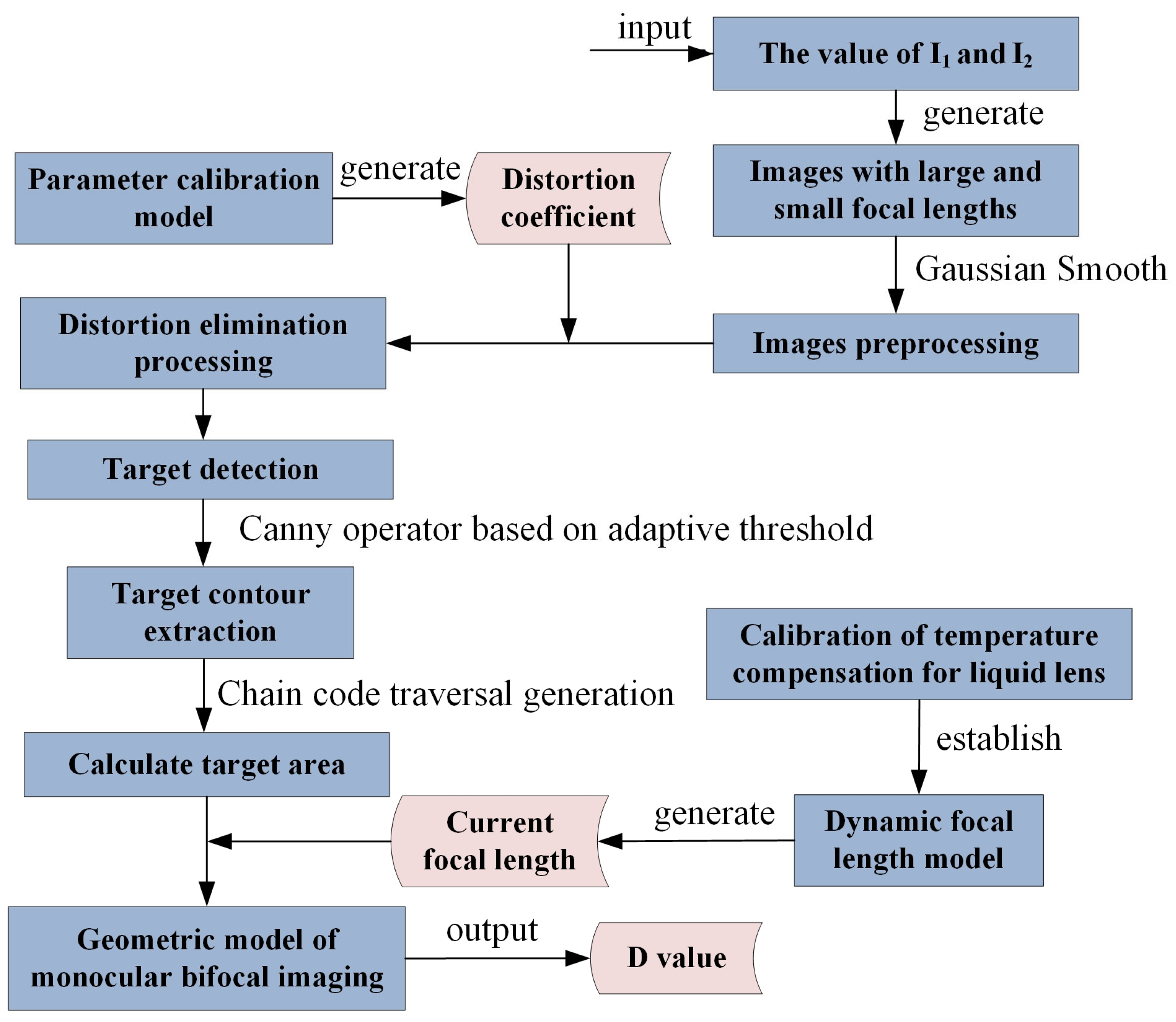
Based on the above parts, a monocular depth sensing method based on liquid zoom imaging is formed, and its algorithm flow is shown in Figure 3. Firstly, by adjusting the input currents I1 and I2 of the two liquid lenses, the system can quickly perform zoom imaging on targets, resulting in two images with wide and narrow fields of view. Then, the image is preprocessed by Gaussian smoothing. According to the distortion coefficient obtained by the system calibration, the object image is processed to eliminate the distortion, and the object contour is extracted by Canny operator based on an adaptive threshold. Furthermore, the area of target images corresponding to wide and narrow fields of view is generated by the calculation method, which is based on chain code classification and strip segmentation. Finally, the dynamic focal length model is adopted to obtain the current focal length of the system, and the target depth D is calculated by combining the monocular bifocal imaging geometric model.

Figure 3.
Flow chart of monocular depth sensing algorithm based on liquid zoom imaging.
3. Experiment and Discussion
3.1. Experimental Method
According to the design configuration in Figure 1, the system platform of monocular depth measurement based on liquid zoom imaging was built, as shown in Figure 4a. The system adopted two pieces of Optotune liquid lenses (beam aperture is 16 mm, focal power can be adjusted from −11D to +11D, response speed is 5 ms, settling time is 20 ms) as optical control devices, which were used to achieve continuous zoom and autofocus of the optical system. The solid-state lens set adopted a fixed focus lens with a focal length of 25 mm, and the sensor adopted a CMOS of model FL-20 (resolution ratio 2736 × 1824, pixel size 4.8 μm). The camera exposure time was set to 4 ms in the experiment.

Figure 4.
Experimental design of monocular depth measurement based on liquid zoom imaging: (a) Physical image of the system platform; (b) Verification plan for measuring performance.
According to the imaging law, the preset current of the liquid lens was given respectively for wide field and narrow field of view. The preset current of wide field of view was −197.73 mA for I1 and 122.86 mA for I2. The preset current of the narrow field of view was 95.18 mA for I1 and −86.82 mA for I2. However, since the focal power of the liquid lens is affected by temperature and target distance, it is necessary to dynamically adjust the current of the liquid lens 1 to keep the image clear. The Tenengrad function was used to evaluate the definition of the target image. If the target image exceeds the standard value, there is no need to focus; otherwise, the autofocus algorithm [15] is invoked to control current I1. The measurement time of the system is the sum of zoom time and autofocus time. Among them, zoom time = response speed of liquid lens + settling time of liquid lens + camera exposure time × 2. Autofocus time ≈ (camera exposure time + response speed of liquid lens + settling time of liquid lens) × number of current adjustments. The performance verification of monocular depth measurement adopts the scheme shown in Figure 4b. The true value of target depth is obtained by laser range finder or high precision scale plate. Measurement relative error = |distance measurement value − distance true value|/distance true value.
3.2. Liquid lens calibration
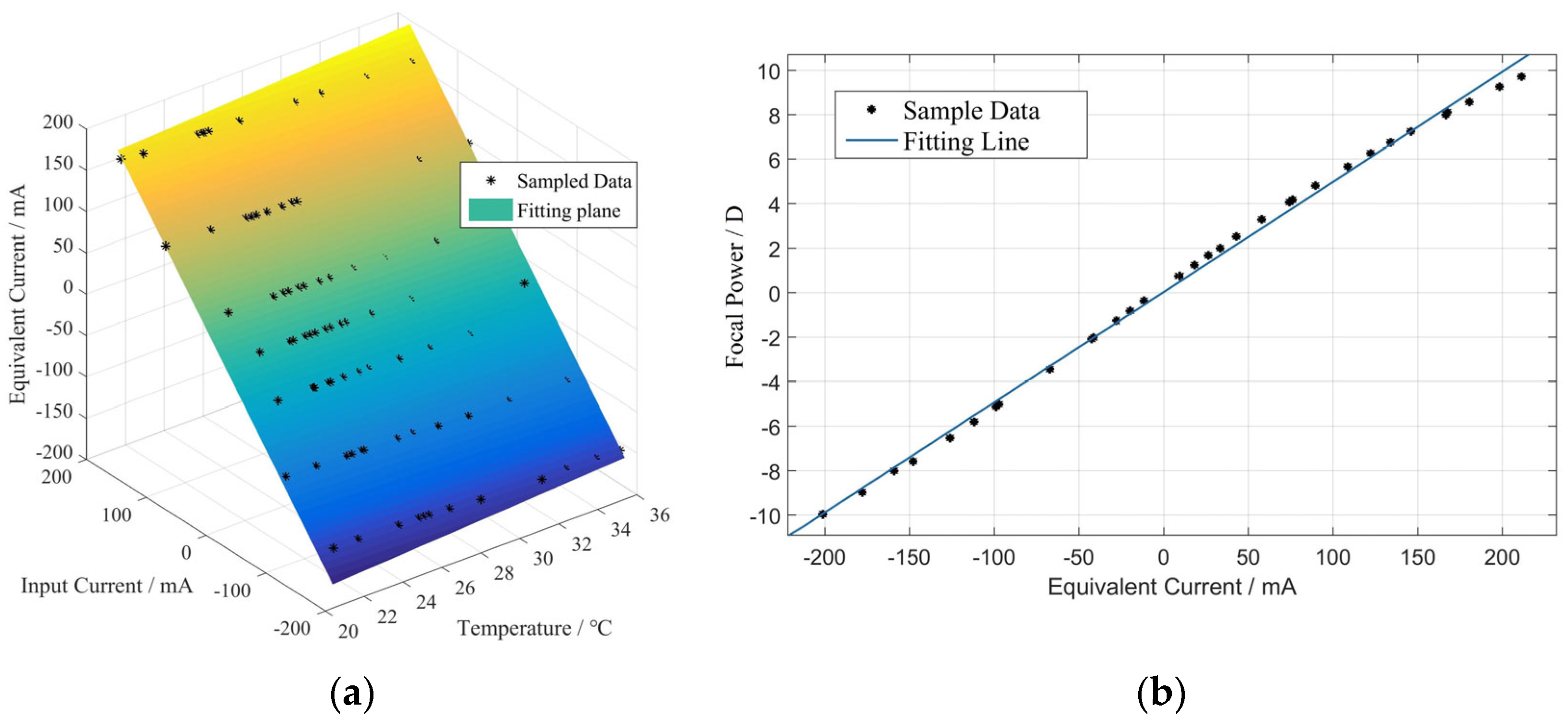
According to the calibration scheme of equivalent current function in Section 2.3.1, the reference temperature was set at 25 °C, and seven groups of data were collected in the range of temperature 21~36 °C and input current −180~180 mA (one group of data with the same focal power, 12 sample data in each group). The focal power of the seven groups was −8D, −5D, −2D, 0.1D, 2D, 5D, and 8D, respectively, then the input current corresponding to the temperature condition of 25 °C was the equivalent current. According to the collected data, the equivalent currents were −158.97 mA, −97.18 mA, −41.12 mA, −2.5 mA, 33.4 mA, 95.68 mA, and 166.69 mA, respectively. With equivalent current–input current–temperature as coordinate axis, the collected data can be converted to three-dimensional coordinates, as shown in Figure 5a. The sampled data are substituted into Equation (5), and the solution result of a was 1.413 by the least square fit algorithm. According to the calibration scheme of the focal power function in Section 2.3.1, 33 samples of input current-temperature-optical focal were obtained based on the sensing information, as shown in Figure 5a. The sampled data were substituted into Equation (6), and the solution results of constants can be obtained by the least square fit algorithm. The values of b and c were 0.04956 and 0.03018, respectively.

Figure 5.
Sample data and fitting results of characteristic parameters of liquid lens: (a) Sampling data and fitting results of input current—temperature—equivalent current; (b) Sampling data and fitting results of equivalent current—focal power.
3.3. System Parameter Determination
According to the distortion coefficient solving method, the distortion coefficients corresponding to the wide and narrow field of view of the system can be obtained, as shown in Table 2.
Table 2.
Solution results of distortion coefficient for the liquid optical system.
Since liquid lens 1 is used for image focusing, the variation of its focal power is affected by both temperature and object distance. However, liquid lens 2 mainly plays a role in changing the focal length of the system, and its focal power change is usually only affected by temperature, so the fluctuation range of the focal power of liquid lens 2 is smaller than the former. Twenty-five groups of data were collected respectively in the preset current neighborhood corresponding to the wide and narrow field of view. According to the data of input current and temperature, the equivalent current and focal power of two liquid lenses were obtained by Equation (6). According to the focal length model solution method in Section 2.3.2, the focal length functions of the system in wide and narrow fields of view can be obtained, as shown in Figure 6.
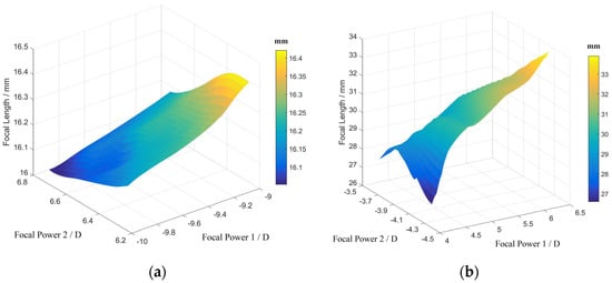
Figure 6.
Solution results of dynamic focal length for liquid optical systems: (a) Wide field of view state; (b) Wide field of view state.
3.4. Target Depth Measurement
3.4.1. Verification of Measurement Accuracy and Efficiency
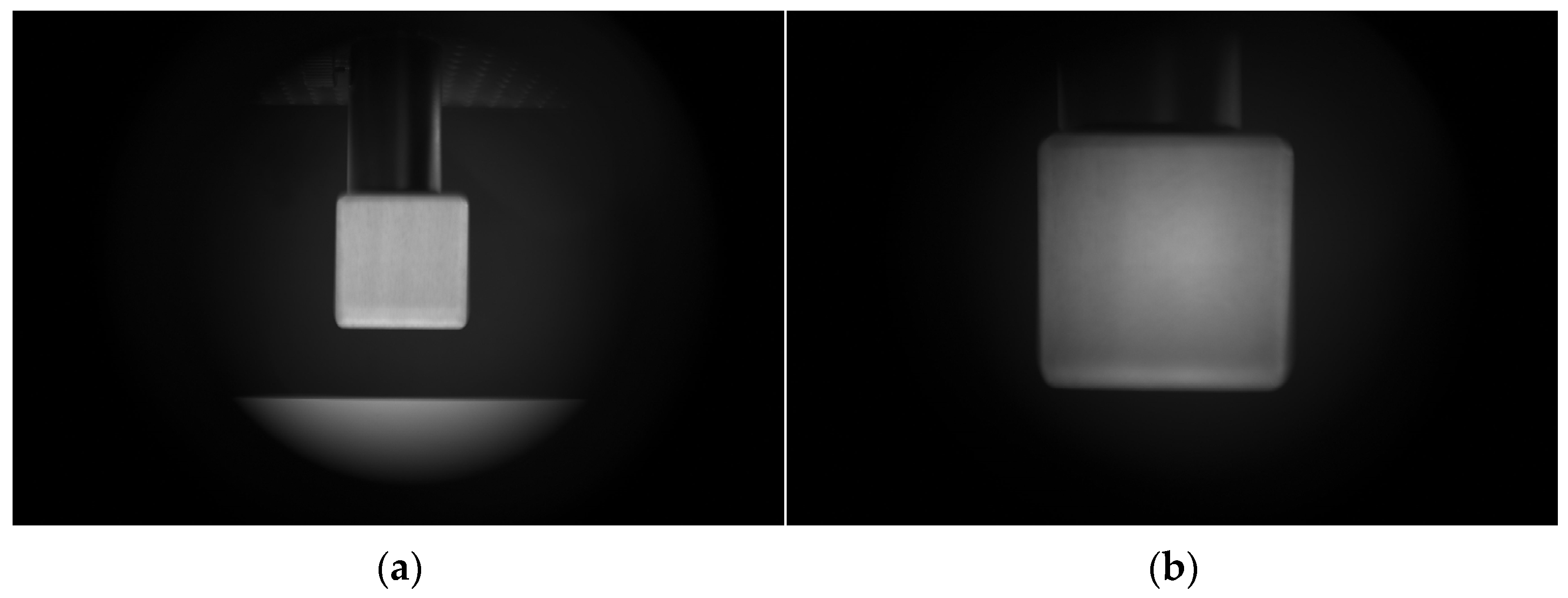
Cube was selected as the test object, and five groups of different object distances (350 mm, 400 mm, 500 mm, 550 mm, and 600 mm) were set for depth measurement experiment. The current focal length is generated from the focal length model based on the real-time parameters of the liquid lens (input current and temperature). For the first group, due to the preset current in the narrow field of view not meeting the image definition requirements, an autofocus algorithm based on liquid lens 1 was initiated. After three times of current adjustment to complete the image focus, the measurement time is 120 ms. Figure 7a,b shows the images taken by the system in wide and narrow fields of view under the first group of object distance conditions. After preprocessing, distortion elimination, edge detection and other processes, the contour extraction results corresponding to wide and narrow fields of view can be obtained, as shown in Figure 7c,d (red part). By combining the computational model with calibration results, the values of S1/S2 and depth D can be generated. For the second group, liquid lens 1 underwent three times of current adjustment to complete the image focus in a narrow field of view, and the measurement time was 120 ms. For groups 3 to 5, due to the preset current to meet the image definition requirements, there is no need to start the autofocus program, and the measurement time was 33 ms.
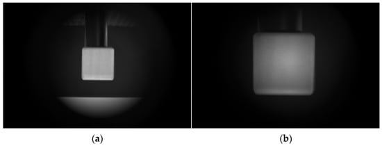
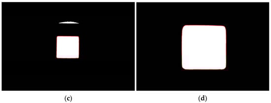
Figure 7.
Imaging results and processing based on liquid optical zoom: (a) Capturing image in the wide field of view state; (b) Capturing image in the narrow field of view state; (c) Target contours corresponding to the wide field of view image; (d) Target contours corresponding to the narrow field of view image.
Table 3 lists the experimental results of the system feature and target depth under five groups of object distance conditions. From the table, it can be seen that the actual measurement error is within the range of 2.90% to 7.05%, with an average value of 4.30%. Since other types of aberrations besides distortion also have coupling effects on the measurement results, there will be some uncertainty in the measurement results of different state targets, resulting in slight fluctuations in the actual measurement errors. The measurement time is within the range of 33 mms to 120 ms, with an average value of 67.8 ms. When the preset current can meet the image definition requirements, the system measurement time is only the zoom time. For example, groups 3 to 5 in Table 3 have the highest measurement efficiency. When the preset current cannot meet the definition requirements of the image, the autofocus algorithm needs to be called, and the measurement time is the sum of the zoom time and the autofocus time. For example, in groups 1 to 2 in Table 3, the measurement efficiency is not as good as the former, and an increase in autofocus time would lead to a decrease in measurement efficiency.
Table 3.
Measurement results of monocular liquid vision under different object distances.
3.4.2. Validation of Generalization Ability
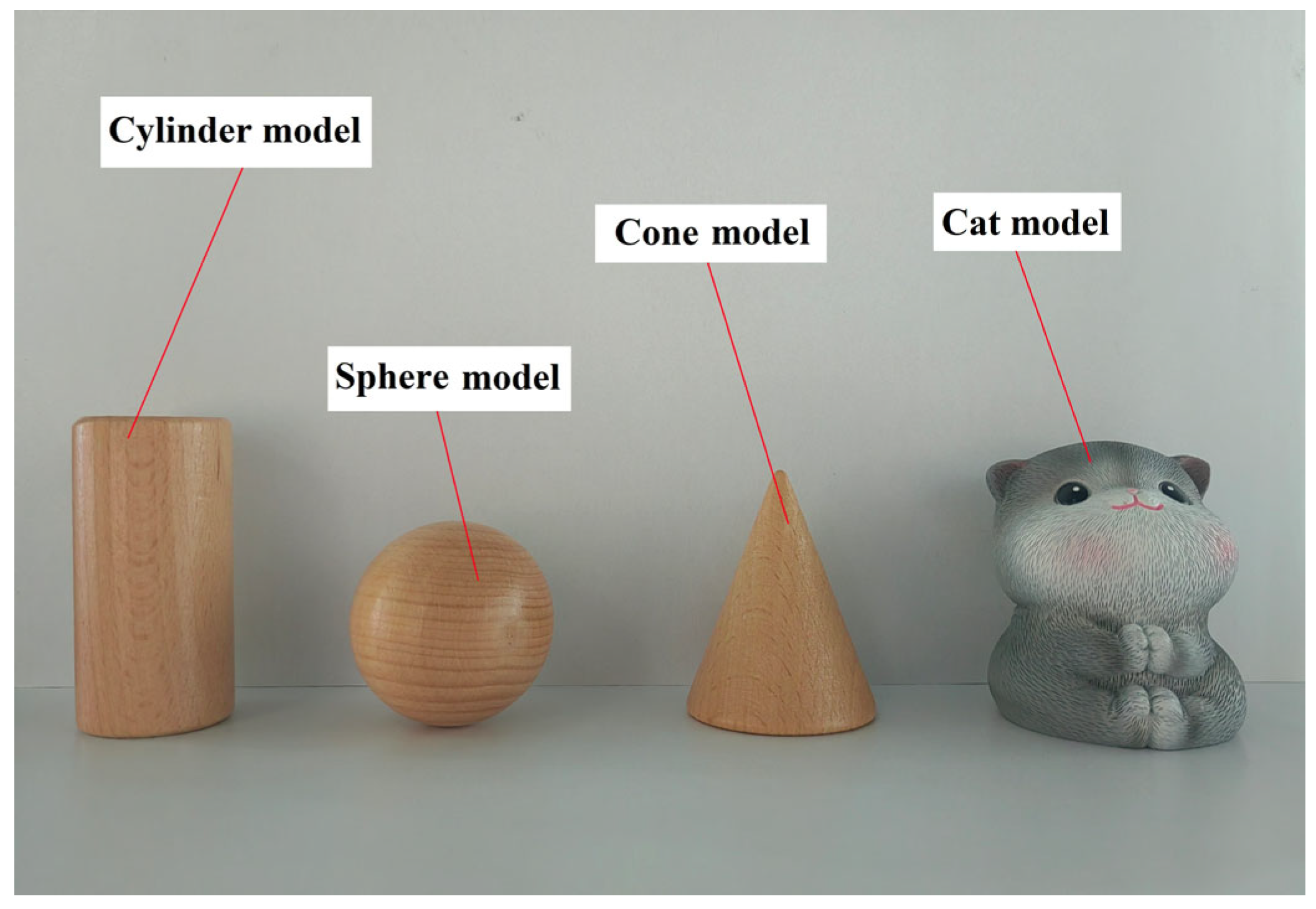
In order to verify the generalization ability of the measurement method, four objects with different shapes (cylinder model, sphere model, cone model, and cat model), as shown in Figure 8, were selected as test objects. The profile section of the measured object was taken as the depth measurement position, and the target distance was set to 500 mm. The liquid vision system was adopted for zoom imaging and image processing, and the depth measurement results were generated based on the proposed algorithm.

Figure 8.
Test objects for generalization validation experiments.
The depth measurement results of four different shaped objects were obtained through testing, as shown in Table 4. It can be seen from the table that the relative measurement error for the four types of targets was less than 5.98%, which indicates that the proposed method has good generalization performance.
Table 4.
Measurement results of monocular liquid vision for objects with different shapes.
4. Conclusions
To summarize, a monocular depth sensing method based on flexible zoom imaging was proposed by combining a liquid zoom mechanism with visual measurement technology. Based on the designed system configuration and working mechanism, a physical platform for a liquid monocular visual measurement system was built. A liquid zoom depth measurement model based on target area invariance was proposed to eliminate the influence of the liquid gravity effect on measurement results, and a target area calculation method based on chain code classification and strip segmentation was given. In response to the fluctuation problem of system focal length caused by factors such as temperature and object distance, a dynamic focal length model of the system was constructed by combining liquid lens calibration. Thus, a whole process method for liquid monocular depth perception was formed, and it was applied to physical platforms for experimental verification. The results show that the monocular depth measurement method based on liquid zoom imaging can achieve high measurement accuracy in the case of unknown target information. Its measurement time can reach the level of ms, and it exhibits good generalization performance for different target shapes. Meanwhile, from the perspective of application scenarios, the method is currently only suitable for measuring close-range targets. The research of this article can provide new ideas for the development of monocular stereo-vision technology.
Author Contributions
Conceptualization, Z.G.; methodology, Z.G.; software, Z.G.; validation, J.L.; formal analysis, M.Z.; investigation, B.L.; resources, Z.G.; data curation, Z.L.; writing—original draft preparation, Z.G.; writing—review and editing, Z.G. and H.H.; supervision, Z.L.; project administration, H.H.; funding acquisition, Z.G. and H.H. All authors have read and agreed to the published version of the manuscript.
Funding
This research was funded by the National Natural Science Foundation of China (Grant No. 62305386) and the Natural Science Foundation of Hunan Province (Grant No. 2022JJ40554).
Data Availability Statement
The data presented in this study are available on request from the author.
Conflicts of Interest
The authors declare no conflicts of interest.
References
- Ma, Y.; Li, Q.; Chu, L.; Zhou, Y.; Xu, C. Real-time detection and spatial localization of insulators for UAV inspection based on binocular stereo vision. Remote Sens. 2021, 13, 230. [Google Scholar] [CrossRef]
- Wang, T.L.; Ao, L.; Zheng, J.; Sun, Z.B. Reconstructing depth images for time-of-flight cameras based on second-order correlation functions. Photonics 2023, 10, 1223. [Google Scholar] [CrossRef]
- Ren, G.; Liu, C.; Liu, P.; Zhang, G. Study on monocular distance measurement based on auto focus. Mach. Des. Manuf. 2019, 4, 146–149. [Google Scholar]
- Kumar, H.; Yadav, A.S.; Gupta, S.; Venkatesh, K.S. Depth map estimation using defocus and motion cues. IEEE Trans. Circuits Syst. Video Technol. 2018, 29, 1365–1379. [Google Scholar] [CrossRef]
- Alenya, G.; Alberich, M.; Torras, C. Depth from the visual motion of a planar target induced by zooming. In Proceedings of the IEEE International Conference on Robotics & Automation, Rome, Italy, 10–14 April 2007; pp. 4727–4732. [Google Scholar]
- Ma, J.; Olsen, S.I. Depth from zooming. J. Opt. Soc. Am. A 1990, 7, 1883–1890. [Google Scholar] [CrossRef]
- Baba, M.; Oda, A.; Asada, N.; Yamashita, H. Depth from defocus by zooming using thin lens-based zoom model. Electron. Commun. Jpn. 2006, 89, 53–62. [Google Scholar] [CrossRef]
- Xu, S.; Wang, Y.; Zhang, Z. 3D reconstruction from bifocus imaging. In Proceedings of the 2010 International Conference on Audio, Language and Image Processing, Shanghai, China, 23–25 November 2010; pp. 1479–1483. [Google Scholar] [CrossRef]
- Huang, A.; Chen, D.; Li, H.; Tang, D.; Yu, B.; Li, J.; Qu, J. Three-dimensional tracking of multiple particles in large depth of field using dual-objective bifocal plane imaging. Chin. Opt. Lett. 2020, 18, 071701. [Google Scholar] [CrossRef]
- Liu, Z.; Hong, H.; Gan, Z.; Xing, K.; Chen, Y. Flexible Zoom Telescopic Optical System Design Based on Genetic Algorithm. Photonics 2022, 9, 536. [Google Scholar] [CrossRef]
- Yoo, N.J.; Kim, W.S.; Jo, J.H.; Ryu, J.M.; Lee, H.J.; Kang, G.M. Numerical calculation method for paraxial zoom loci of complicated zoom lenses with infinite object distance by using Gaussian bracket method. Korean J. Opt. Photonics 2007, 18, 410–420. [Google Scholar] [CrossRef]
- Liu, C.; Zheng, Y.; Yuan, R.Y.; Jiang, Z.; Xu, J.B.; Zhao, Y.R.; Wang, X.; Li, X.W.; Xing, Y.; Wang, Q.H. Tunable liquid lenses: Emerging technologies and future perspectives. Laser Photonics Rev. 2023, 17, 2300274. [Google Scholar] [CrossRef]
- Yang, P.; Song, W.; Zhao, X.; Zheng, R.; Qingge, L. An improved Otsu threshold segmentation algorithm. Int. J. Comput. Sci. Eng. 2020, 22, 146–153. [Google Scholar] [CrossRef]
- Annapurna, P.; Kothuri, S.; Lukka, S. Digit recognition using freeman chain code. Int. J. Appl. Innov. Eng. Manag. 2013, 2, 362–365. [Google Scholar]
- Liu, Z.; Hong, H.; Gan, Z.; Xing, K. Bionic vision autofocus method based on a liquid lens. Appl. Opt. 2022, 61, 7692–7705. [Google Scholar] [CrossRef] [PubMed]
- Li, Y.; Wang, G.; Wang, Y.; Cheng, Z.; Zhou, W.; Dong, D. Calibration method of liquid lens focusing system for machine vision measurement. Infrared Laser Eng. 2022, 51, 20210472. [Google Scholar]
- Ricolfe-Viala, C.; Sanchez-Salmeron, A.J. Lens distortion models evaluation. Appl. Opt. 2010, 49, 5914–5928. [Google Scholar] [CrossRef] [PubMed]
- Choi, B.K.; Yoo, W.S.; Lee, C.S. Matrix representation for NURB curves and surfaces. Comput. Aided Des. 1990, 22, 235–240. [Google Scholar] [CrossRef]
- Bradley, C.H.; Vickers, G.W. Free-form surface reconstruction for machine vision rapid prototyping. Opt. Eng. 1993, 32, 2191–2200. [Google Scholar] [CrossRef]

Disclaimer/Publisher’s Note: The statements, opinions and data contained in all publications are solely those of the individual author(s) and contributor(s) and not of MDPI and/or the editor(s). MDPI and/or the editor(s) disclaim responsibility for any injury to people or property resulting from any ideas, methods, instructions or products referred to in the content. |
© 2024 by the authors. Licensee MDPI, Basel, Switzerland. This article is an open access article distributed under the terms and conditions of the Creative Commons Attribution (CC BY) license (https://creativecommons.org/licenses/by/4.0/).