Revisiting Poincaré Sphere and Pauli Algebra in Polarization Optics

Abstract

We present one of the main lines of development of Poincaré sphere representation in polarization optics, by using largely some of our contributions in the field. We refer to the action of deterministic devices, specifically the diattenuators, on the partial polarized light. On one hand, we emphasize the intimate connection between the Pauli algebraic analysis and the Poincaré ball representation of this interaction. On the other hand, we bring to the foreground the close similarity between the law of composition of the Poincaré vectors of the diattenuator and of polarized light and the law of composition of relativistic admissible velocities. These two kinds of vectors are isomorphic, and they are “imprisoned” in a sphere of finite radius, standardizable at a radius of one, i.e., Poincaré sphere.

1. Introduction: Early Days of the Poincaré Sphere

In the last chapter (XII, §158) of his Théorie Mathématique de la Lumière [1], Henri Poincaré raised a stereographic projection of the circle of radius one of the complex plane for obtaining an equivalent real tridimensional representation, on a sphere of radius one, of the complex representation of the manifold of polarization states. This was the birth of the celebrated Poincaré sphere. At that time, it was only about what we name today pure polarization states [2], namely those represented by points on the surface of the sphere.

Of course, Poincaré was aware of the Riemann sphere. On the other hand, Poincaré sphere is the precursor of the Bloch sphere, which constitutes the tridimensional representation of the pure state space of any two-level quantum system (we know today that the pure polarization states constitute a two-level system [2]).

Poincaré used this spherical representation for describing the transformation of optical polarization states (SOPs) under the action of various retarders and the succession of retarders. Well known, the retarders (phase-shifters) are only polarization form converters, such that Poincare’s analyses were limited to the surfaces of the sphere. He has not presented an image of the sphere; merely, he has described in words what passes with the polarization states on it.

Probably, the first textbook in which the Poincaré sphere appears in the form we are accustomed with is the bibliographically exhaustive, for that time, Shurcliff ’s Polarized Light [3]. For us, the theory of light polarization is in a great measure a question of non-abelian linear algebra (in matrix, quaternionic, or other forms), sometimes burdened by the complexity of the corresponding mathematics. Shurcliff’s book has the ancient flower of the intuitive connection between the mathematical descriptions and the physical essence of the described phenomena. Concerning the Poincaré sphere: “Despite his great usefulness, it has been given little attention in the literature. The writer has been unable to find any substantial account of it in any textbook. Brief description of it appeared in a number of technical journals”. In 1962, Shurcliff remains within Poincaré’s limits: “The method is applicable only if the incident state is completely polarized”—i.e., on the surface of the sphere ([3], p. 17).

Nevertheless, even earlier, and even in the quoted papers, substantial progress has been made. Jerrard [4] has given a clear theory and representation of the states on the Poincaré sphere, but also referring only to its surface. Fano [5] and MacMaster [6] recognized the partially polarized SOPs as mixed states and represented them as polar vectors inside the Poincaré sphere. Ramachandran and Ramaseshan [7] presented in detail the properties of the Poincaré representation and applied it in the propagation of the totally and partially polarized light through various birefringent and dichroic crystals. They underlined that the partially polarized SOPs may be associated with points inside the Poincaré sphere (in the “Poincaré ball”) and defined the Poincaré vectors of the SOPs as their normalized Stokes vectors ([7], pp. 18–19). Thus, they fully brought to light all the capacities of “this representation admirably suited for the purpose of analyzing the changes in the state of polarization of a beam of light traversing an anisotropic medium” ([7], p. 2).

Among the classical textbooks which give a clear illustration of the Poincaré sphere, raising it by the stereographic projection from the circular complex plane representation of the polarization states, is Azzam and Bashara’s book ([8], pp. 47–51). This book is singular in giving an exhaustive treatment of the polarized light in terms of complex plane representation, but, at the same time, it provides many expressive connections with the Poincaré representation.

For all the general references, we refer to the textbook by J. J. Gill and R. Ossikovski [2], which, generally in a Mueller matrix approach, also provides an update on the problem of various geometric Poincaré representations in the polarization theory.

In this paper, we will present a line of modern development of the Poincaré representation, underlying its connections with the Pauli algebra of 2 × 2 operators and with some aspects of the special theory of relativity, and emphasizing its expressivity in the problems of interaction of partially polarized light with dichroic devices, e.g., the enpolarization/depolarization given by these devices.

2. The Poincaré Vectors of Partially Polarized Light and of Dichroic Devices

Until now, we have seen how the representation of the pure polarization states on the sphere was extended to the representation of the mixed states in the Poincaré ball. Each SOP corresponds with a polar vector (with the tail at the center of the sphere), whose direction indicates the polarization form and whose modulus gives the degree of light polarization. The next step in developing the Poincaré paradigm is to extend it to the polarization devices. We shall see that to each deterministic device [2] one can associate a (device) Poincaré vector. We have to note, from the beginning, that while the Poincaré space is isomorphic with manifold of all the SOPs, it is isomorphic only with the manifold of deterministic polarization devices.

In the following, we shall refer only to the dichroic devices (more precisely to orthogonal diattenuators) [9]. Notably, these devices are represented by Hermitian operators, which, together with the unitary operators representing the phase-shifters, constitute the building blocks of any deterministic normal operator. The phase-shifters have a very simple action in the Poincaré ball, they simply rotate any SOP around their Poincaré axes; they do not create any special problem. On the contrary, the action of the diattenuators is much more complex, namely their Poincaré vectors are composed with those of the SOPs in a complicated way, similar to that of relativistic velocities. Therefore, the various aspects of their action throw a fresh light on the various counterintuitive aspects of the relativistic boost, which is one of the goals of this paper.

Certainly, the most widespread mathematical representation of the polarization devices is that of the classical matrices. Here, we shall use the Pauli algebraic representation of SOPs and deterministic devices because it is the most directly connected with the Poincaré geometric representation. The Pauli algebraic representation was introduced by C. Withney [10], based on the suggestion of Prof. L Tisza, in a program, at MIT, for developing the physical applications of Pauli algebra. At that time a young top algebraist, Chyntia Withney is now one of the leaders of the dissident movement in the theory of special relativity [11]. Shih-Yau Lu and R. A. Chipman, at the beginning of their seminal paper [12], give the Pauli expansion of a diattenuator ([12], Equation (7)) and define “the axis of the diattenuator to be the eigenpolarization with the larger eigenvalue”. It is easy to see, under the c_i coefficients of this Pauli expansion, the normalized Stokes parameters of the dichroic device. As we shall see the “axis of the diattenuator” is also the Pauli axis of its operator and the Poincaré axis of its representation in the Poincaré ball.

Between the Pauli algebraic expressions of the operators of the completely polarized light and of an ideal polarizer, there is a perfect symmetry [2]:

$$\mathrm{J}=\frac{1}{2}({\sigma }_0+s.\sigma )$$

(1)

$$\mathrm{P}=\frac{1}{2}({\sigma }_0+z.\sigma )$$

(2)

Here, ${\sigma }_0$ and $\sigma$ are the unit 2 × 2 matrix and the Pauli matrix vector $\sigma ({\sigma }_1,{\sigma }_2,{\sigma }_3)$:

$${\sigma }_0=\left(\begin{array}{cc}1& 0\\ 0& 1\end{array}\right)\hspace{0.17em}\hspace{0.17em}\hspace{0.17em}{\sigma }_1=\left(\begin{array}{cc}0& 1\\ 1& 0\end{array}\right),\hspace{0.17em}\hspace{0.17em}\hspace{0.17em}{\sigma }_2=\left(\begin{array}{cc}0& -i\\ i& 0\end{array}\right),\hspace{0.17em}\hspace{0.17em}\hspace{0.17em}{\sigma }_3=\left(\begin{array}{cc}1& 0\\ 0& -1\end{array}\right)$$

(3)

In Equations (1) and (2), $\mathrm{J}$ is the density operator (in matrix language, the coherency matrix or the polarization-coherency matrix [2]) of the polarized light, and $\mathrm{P}$ the operator of the device. The vectors $\mathbf{s}$ and $\mathbf{z}$ are the so-called Pauli axes (or Pauli vectors) of the corresponding operators. They correspond directly to the Poincaré vectors of the pure SOP and of the ideal (generally elliptic) polarizer, respectively. Thus, to each state of totally polarized light corresponds an ideal polarizer and vice-versa. Particularly, each state of totally polarized light may be produced, from unpolarized light, by the corresponding ideal polarizer. Similarly, a diattenuator acting on unpolarized light gives partially polarized light whose polarization parameters reproduce (disclose) the polarization parameters of the device.

For partially polarized light, its density operator (normed at unity) is [2]:

$$\mathrm{J}=\frac{1}{2}({\sigma }_0+p_l{\mathbf{n}}_l.\sigma )$$

(4)

where $p_l$ is the degree of light polarization, and ${\mathbf{n}}_l$ is the unit vector corresponding to its form of polarization, so that $p_l{\mathbf{n}}_l$ is the Poincaré vector of any polarization state (pure or mixed) at this time. While the top of the Poincaré axis ${\mathbf{n}}_l$ of the state lies on the Poincaré sphere ${\Sigma }_2^1$, the top of its Poincaré vector $p_l{\mathbf{n}}_l$ lies in the Poincaré ball ${\Sigma }_3^1$, on the sphere of radius $p_l$, ${\Sigma }_2^{p_l}$ (the lower index stands for the dimensionality of the space: 2—the surface of the sphere, and 3—solid sphere, ball; the upper index for the radius of the sphere or the ball).

In regard to the diattenuators, their characteristics are the principal (eigen) transmittances $e^{{\eta }_1}$ and $e^{{\eta }_2}$, where ${\eta }_1$ and ${\eta }_2$ are the coefficients of extinction ([7], p. 14; [8], pp. 74–76). Both eigen transmittances are defined at the level of light wave amplitude. But the characteristic of the diattenuators that we are accustomed to—the diattenuation—is defined at the level of intensity:

$$\mathfrak{D}=\frac{{\left|e^{{\eta }_1}\right|}^2-{\left|e^{{\eta }_2}\right|}^2}{{\left|e^{{\eta }_1}\right|}^2+{\left|e^{{\eta }_2}\right|}^2}$$

(5)

In (5), we have preserved the original form of the definition of the diattenuation, as cited in [12]; evidently, the moduli in this definition have sense when the device is not a pure diattenuator, i.e. when it has also birefringence.

Apparently, the diattenuation contains, in an inextricably way, the isotropic transmittance of the device together with the truly anisotropic aspect of the transmittance. But let us denote:

$$\frac{{\eta }_1+{\eta }_2}{2}=\rho \mathrm{and}{\eta }_1-{\eta }_2=\eta$$

(6)

where $\eta$ directly reflects the anisotropy at the level of the coefficients of extinction. Then,

$$e^{{\eta }_1}=e^{\rho }{e}^{\frac{\eta }{2}},e^{{\eta }_2}=e^{\rho }{e}^{-\frac{\eta }{2}}$$

(7)

and coming back to the definition of the diattenuation, we get:

$$\mathfrak{D}=\frac{e^{\eta }-e^{-\eta }}{e^{\eta }+e^{-\eta }}=\tanh \eta$$

(8)

An equivalent term well suited for our purpose of Poincaré ball analysis is the degree of dichroism (or even the dichroic strength) of the diatenuator:

$${\mathrm{p}}_d\equiv \mathfrak{D}=\tanh \eta$$

(9)

Like the tanh function,

$${\mathrm{p}}_d\in [0,1],$$

(10)

namely, from 0 for an isotropic device $({\eta }_1={\eta }_2,\hspace{0.17em}\eta =0)$ and, at the limit, to 1 for an ideal polarizer (${\eta }_1\hspace{0.17em}\to \hspace{0.17em}0,\hspace{0.17em}{\eta }_2\hspace{0.17em}\to \hspace{0.17em}-\infty ,\hspace{0.17em}\eta \hspace{0.17em}\to \hspace{0.17em}\infty$).

Keeping in mind this analogy between the characteristics of the partially polarized light and those of the diattenuators, these devices can be represented, as well as the SOPs, by polar vectors in the Poincaré ball, pointing in the direction $n_d$ corresponding to their form (linear, circular, and various elliptical diattenuators), and of modulus $p_d$ corresponding to their degree of dichroism (diattenuation, dichroic strength). We shall take the Pauli/Poincaré axis of the dichroic device $n_d$ as corresponding to its major eigenstate (defined as the state of maximum transmittance). A classical matrix approach to the analogy between the algebraic descriptions of SOPs and of the devices is given in [13].

Henceforth, we will use a unitary notation for SOPs and diattenuators, namely, ${\mathbf{s}}_i=p_i{\mathbf{n}}_i$, ${\mathbf{s}}_d=p_d{\mathbf{n}}_d$, and ${\mathbf{s}}_o=p_o{\mathbf{n}}_o$, where the vectors s represent the Poincaré vectors and n the Poincaré axes (unit vectors) of the SOPs and of the device, $p$ is the degree of polarization of the SOP or the degree of dichroism of the device, and indices i, d, o stand for incident light, device, and emergent (output) light, respectively. The (SOP’s or devices’) Poincaré axes or vectors in the Poincaré ball are the same as those in the Pauli algebraic expressions of the corresponding operators. For this reason, when one presents the evolution of the Poincaré paradigm, it is by far more adequate to address the Pauli algebraic compact form of the operators. They are directly and intimately connected.

3. Action of a Diattenuator on Partially Polarized Light: The Composition Law of the Poincaré Vectors of a Diattenuator and of Incident Polarized Light

The action of the device on the polarized light may be analyzed at the level of the light spinor (Jones vector) only for the pure states. For mixed states, it can be analyzed at the level of the density operator of the state, where it takes the operatorial form [2]:

$${\mathrm{J}}_o=\mathrm{D}{\mathrm{J}}_i{\mathrm{D}}^{†}$$

(11)

Let us consider the action of a diattenuator on the partially coherent light. The operator of the diattenuator is a Hermitian one and may be written as follows [14,15]:

$${\mathrm{H}}_d(\rho ,\eta )=\frac{1}{2}{e}^{\rho }({\sigma }_0\cosh \frac{\eta }{2}+n_d.\sigma \sinh \frac{\eta }{2})$$

(12)

where $n_d$ is its Pauli, or Poincaré, axis, and $\rho$ and $\eta$ are given by Equation (6). If one prefers the classical (not Pauli-compacted) Jones calculus, by choosing a particular axis of the diattenuator, one readily obtains the Jones forms of the (e.g., linear or circular) diattenuators, whose presence in the literature goes back to the fundamental Jones papers [16].

With Equations (4) and (12) substituted in (11) we obtain the following [17]:

$$\begin{gathered} {\mathrm{J}}_o={\mathrm{H}}_d(\rho ,\eta ){\mathrm{J}}_i {\mathrm{H}}_d^{†}(\rho ,\eta ) \\ =\frac{1}{2}{e}^{2\rho }({\sigma }_0\cosh \frac{\eta }{2}+n_d.\sigma \sinh \frac{\eta }{2})({\sigma }_0+p_i{\mathbf{n}}_i.\sigma )({\sigma }_0\cosh \frac{\eta }{2}+n_d.\sigma \sinh \frac{\eta }{2}) \end{gathered}$$

(13)

$${\mathrm{J}}_o=\frac{1}{2}{e}^{2\rho }(\cosh \eta +p_i{\mathbf{n}}_i.{\mathbf{n}}_d\sinh \eta )\left[{\sigma }_0 +\frac{p_i{\mathbf{n}}_i+{\mathbf{n}}_d\sinh \eta +2p_i({\mathbf{n}}_d.{\mathbf{n}}_i){\mathbf{n}}_d {\sinh }^2\frac{\eta }{2}}{\cosh \eta +p_i{\mathbf{n}}_i.{\mathbf{n}}_d\sinh \eta }\sigma \right]$$

(14)

This expression is that of a mixed state:

$${\mathrm{J}}_o=\frac{1}{2}g\left[{\sigma }_0 +p_o{s}_o.\sigma \right]$$

(15)

where g is the gain given by the dichroic device:

$$g=e^{2\rho }(\cosh \eta +p_i{\mathbf{n}}_i.{\mathbf{n}}_d\sinh \eta )$$

(16)

and the Poincaré vector of the output light is given by:

$$p_o{\mathbf{n}}_o=\frac{p_i{\mathbf{n}}_i+{\mathbf{n}}_d\sinh \eta +2p_i({\mathbf{n}}_d.{\mathbf{n}}_i){\mathbf{n}}_d{\sinh }^2\frac{\eta }{2}}{\cosh \eta +p_i{\mathbf{n}}_i.{\mathbf{n}}_d\sinh \eta }$$

(17)

It is worth mentioning that, in a Pauli algebraic approach, all the characteristics (gain, Poincaré vector, i.e., Poincaré axis, and degree of polarization) of the output light are provided in block and firmly separated one with the other. In the classical matrix approach, often they are entangled ( e.g., Azzam and Bashara’s note at (p. 145 [8]) on a well-known “elegant” expression of the gain). As a little digression, Equation (16) of the gain leads directly to a very expressive form of the generalized Malus’ law [18], but which has little relevance to the Poincaré sphere. On this sphere, of fixed radius (conventionally one), we can address only problems of polarization states.

Thus, let us look further into Equation (17). It expresses a connection between the Poincaré vectors of the output SOP, ${\mathbf{s}}_o=p_o{\mathbf{n}}_o$, and of the input SOP, ${\mathbf{s}}_i=p_i{\mathbf{n}}_i$, in which the characteristic elements of the diattenuator appear mingled. Its Poincaré axis, ${\mathbf{n}}_d$, appears, its degree of polarization, $p_d$, does not; but, in this respect, we have at hand the basic Equation (9). Evidently, when dealing with dichroic devices, we use full hyperbolic trigonometry and geometry, and, in processing further Equation (17), we have to use the relationships between the hyperbolic functions. We could continue on this inductive way, changing the unexpressive (in this context) hyperbolic parameter $\eta$ with the degree of dichroism, $p_d$, all the more since $cosh \eta$ also leads to something expressive:

$$\hspace{0.17em}\cosh \eta =\frac{1}{\sqrt{1-{\tanh }^2\eta }}=\frac{1}{\sqrt{1-p_d^2}}={\gamma }_d$$

(18)

But this inductive way has been discussed, not easily, in another field in which we owe so much to Henri Poincaré, namely, in the special theory of relativity (STR). Thus, let us to have a stop and look at the problem from a higher perspective.

The Poincaré vectors of the input SOP, the output SOP, and the diattenuator are, all, modulus limited to unity, because neither the degree of polarization nor the degree of dichroism can overpass unity:

$${\mathbf{s}}_d,{\mathbf{s}}_i,{\mathbf{s}}_o\in ({ℝ}^3;\left|{\mathbf{s}}_d\right|=p_d,\left|{\mathbf{s}}_i\right|=p_i,\left|{\mathbf{s}}_o\right|=p_o\le 1)$$

(19)

The polar Poincaré vectors ${\mathbf{s}}_i=p_i{\mathbf{n}}_i$ and ${\mathbf{s}}_d=p_d{\mathbf{n}}_d$ (with the tails at the center of the sphere) must be composed in such a way that their result, ${\mathbf{s}}_o=p_o{\mathbf{n}}_o$, should remain (with the same tail) in the Poincaré ball. Evidently, this is another rule of “adding” than the parallelogram rule corresponding to classical vectors. But this rule was already invented and, for a long time, elaborated in detail in the special theory of relativity. The relativistic admitted velocities are vectors of the same kind as the Poincaré vectors, and for:

$$\mathbf{u},\mathbf{v},\mathbf{w}\in ({ℝ}^3;\left|\mathbf{u}\right|,\left|\mathbf{v}\right|,\left|\mathbf{w}\right|\le 1)$$

(20)

their most general composition law has the form [19,20]:

$$\mathbf{w}=\mathbf{u}\oplus \mathbf{v}=\frac{\mathbf{u}+\mathbf{v}}{1+\mathbf{u}\mathbf{.}\mathbf{v}}+\frac{{\gamma }_u}{{\gamma }_u+1}\frac{\mathbf{u}\times (\mathbf{u}\times \mathbf{v})}{1+\mathbf{u}\mathbf{.}\mathbf{v}}$$

(21)

with ${\gamma }_u$ the “Lorentz factor” associated with the boost $\mathbf{u}$:

$${\gamma }_u=\frac{1}{\sqrt{1-u^2}}$$

(22)

Hungar has shown that these vectors form a pseudo-group (deprived of commutativity) and coined for them the name “gyrovectors” [19].

Applied to the Poincaré polarization vectors, this rule of composition should look as follows:

$${\mathbf{s}}_o={\mathbf{s}}_d\oplus {\mathbf{s}}_i=\frac{{\mathbf{s}}_d+{\mathbf{s}}_i}{1+{\mathbf{s}}_d.{\mathbf{s}}_i}+\frac{{\gamma }_d}{{\gamma }_d+1}\frac{{\mathbf{s}}_d\times ({\mathbf{s}}_d\times {\mathbf{s}}_i)}{1+{\mathbf{s}}_d.{\mathbf{s}}_i}$$

(23)

or equivalently:

$$p_o{\mathbf{n}}_o=\frac{p_i{\mathbf{n}}_i+p_d{\mathbf{n}}_d}{1+(p_i{\mathbf{n}}_i)\mathbf{.}(p_d{\mathbf{n}}_d)}+\frac{{\gamma }_d}{{\gamma }_d+1}\frac{p_d{\mathbf{n}}_d\times (p_d{\mathbf{n}}_d\times p_i{\mathbf{n}}_i)}{1+(p_i{\mathbf{n}}_i)\mathbf{.}(p_d{\mathbf{n}}_d)}$$

(24)

with

$${\gamma }_d=1/\sqrt{1-p_d^2}$$

(25)

the “Lorentz factor” of the diattenuator.

Let us verify whether Equations (17) and (24) are indeed equivalent. For this purpose, we first process Equation (17):

$$\begin{gathered} p_o{\mathbf{n}}_o=\frac{p_i{\mathbf{n}}_i+{\mathbf{n}}_d\sinh \eta +p_i(\cosh \eta -1){\mathbf{n}}_d({\mathbf{n}}_d\mathbf{.}{\mathbf{n}}_i)}{\cosh \eta +p_i{\mathbf{n}}_i\mathbf{.}{\mathbf{n}}_d\sinh \eta } \\ =\frac{p_i{\mathbf{n}}_i+{\mathbf{n}}_d\tanh \eta +p_i(1-1/\cosh \eta )\left[{\mathbf{n}}_d({\mathbf{n}}_d\mathbf{.}{\mathbf{n}}_i)-{\mathbf{n}}_i\right]}{1+p_i{\mathbf{n}}_i\mathbf{.}{\mathbf{n}}_d\tanh \eta } \end{gathered}$$

(26)

With Equations (9) and (25), Equation (26) becomes the following:

$$p_o{\mathbf{n}}_o=\frac{p_i{\mathbf{n}}_i+p_d{\mathbf{n}}_d}{1+(p_i{\mathbf{n}}_i)\mathbf{.}(p_d{\mathbf{n}}_d)}+\frac{{\gamma }_d}{{\gamma }_d+1}\frac{p_i{p}_d^2\left[{\mathbf{n}}_d({\mathbf{n}}_d\mathbf{.}{\mathbf{n}}_i)-{\mathbf{n}}_i\right]}{1+(p_i{\mathbf{n}}_i)\mathbf{.}(p_d{\mathbf{n}}_d)}$$

(27)

which can be easily expressed in the form of Equation (24).

Mathematically, the restrictions (19)–(20) are equivalent, as well as their consequences, Equations (24) and (21), but from an epistemological view point, they are not. The rule of composition of relativistic admissible velocity is “bizarre and counterintuitive” [20] because of the basic counter intuitiveness of the second postulate, which imposes the restriction (20) and leads to the well-known paradoxes of the special theory of relativity. (In paper [20], Hungar analyzes one of the less mentioned paradoxes, namely, the Mocanu’s paradox.) With respect to the restriction (19), it is not counterintuitive, it has a simple and natural reason: non-overpolarizability. If its consequence (24) would have been established first (e.g., on the inductive way, as described above), our understanding of this kind of vectors (the gyrovectors) would have naturally made more sense.

In the following sections, we will mention some consequences of the rule of composition (24).

4. The Effect of a Diattenuator on an Individual SOP

As the first step, let us see what becomes of this “gyrocomposition law” in some particular simple cases.

If the Poincaré vector of the diattenuator is parallel with that of the incident SOP (${\mathbf{s}}_d\uparrow \uparrow {\mathbf{s}}_i$; ${\mathbf{n}}_d\equiv {\mathbf{n}}_i$), the last term in Equation (24) vanishes and one obtains the following:

$$p_o{\mathbf{n}}_o=\frac{p_i+p_d}{1+p_i{p}_d}{\mathbf{n}}_i \left[p_o=\frac{p_i+p_d}{1+p_i{p}_d}\right]$$

(28)

The Poincaré axis of the light SOP is conserved after passing through the diattenuator.

If the Poincaré vector of the diattenuator is antiparallel with that of the incident SOP (${\mathbf{s}}_d\uparrow \downarrow {\mathbf{s}}_i$; ${\mathbf{n}}_d=-{\mathbf{n}}_i$), Equation (24) gives:

$$p_o{\mathbf{n}}_o=\frac{p_i-p_d}{1-p_i{p}_d}{\mathbf{n}}_i\hspace{0.17em}\hspace{0.17em}\hspace{0.17em}\hspace{0.17em}{p}_o=\frac{\left|p_i-p_d\right|}{1-p_i{p}_d}$$

(29)

The antiparallelism of Poincaré vectors of the SOP and of the device means that their major axes point towards the opposite points of the sphere, e.g., for fixing ideas, ${\mathbf{n}}_i$, towards the north pole, and ${\mathbf{n}}_d$ towards the south pole. Then, the polarization structures of the incident light SOP and of the device are antagonistic; the incident light is (generally partially) right circularly polarized, and the diattenuator is a left circular one. The (orientation of the Poincaré axis of the) emergent light SOP will be decided by the “competition” between the strength of the diattenuator and that of the incident SOP (${\mathbf{n}}_o={\mathbf{n}}_d=-{\mathbf{n}}_i$, if $p_d>p_i$; and ${\mathbf{n}}_o={\mathbf{n}}_i$ for $p_i>p_d$). If this antagonistic case is balanced ($p_d=p_i$), the diattenuator depolarizes completely the incident light ($p_o=0$).

If the incident light is unpolarized ($p_i=0$, ${\mathbf{n}}_i$ undefined), the emergent light will be polarized in the major state of the diattenuator (${\mathbf{n}}_o={\mathbf{n}}_d$), with a degree of polarization equal to the degree of dichroism of the device. The unpolarized incident light “extracts” from the device and “uncovers” its polarization structure.

Equations (28) and (29) correspond to the rules of adding the relativistic admissible parallel or antiparallel velocities in theory of special relativity, which are known for more than one century. But while all their consequences described above are very natural, the corresponding STR rules remain “bizarre and counterintuitive”, as at the beginning, because their root, the second postulate, remains counterintuitive despite all the great mathematics in which it was shrouded. It does not disturb us the fact that, if either the incident light is totally polarized or the diattenuator becomes a pure polarizer ($p_d=1$), in both the previous cases, the output light is totally polarized ($p_i=1$ and $p_d=1$ $\Rightarrow$ $p_o=1$). But we are annoyed by the fact that, in STR, for the parallel velocity composition, c + v = c.

The point that needs to be emphasized is that the polarization Poincaré vectors do not constitute the only case in physics where the gyrovector composition law works “naturally”. In 1992, Vigoureux [21] showed that the same composition law can be applied to the study of multilayers (in this first paper, he has referred to the parallel vector composition law of STR). This is connected with the fact that the reflection coefficients are modulus limited at the value of one. Even if this perspective in the field of multilayers has rapidly widened, it has not taken advantage of the Poincaré vectorial representation, and it remained in an algebraic frame.

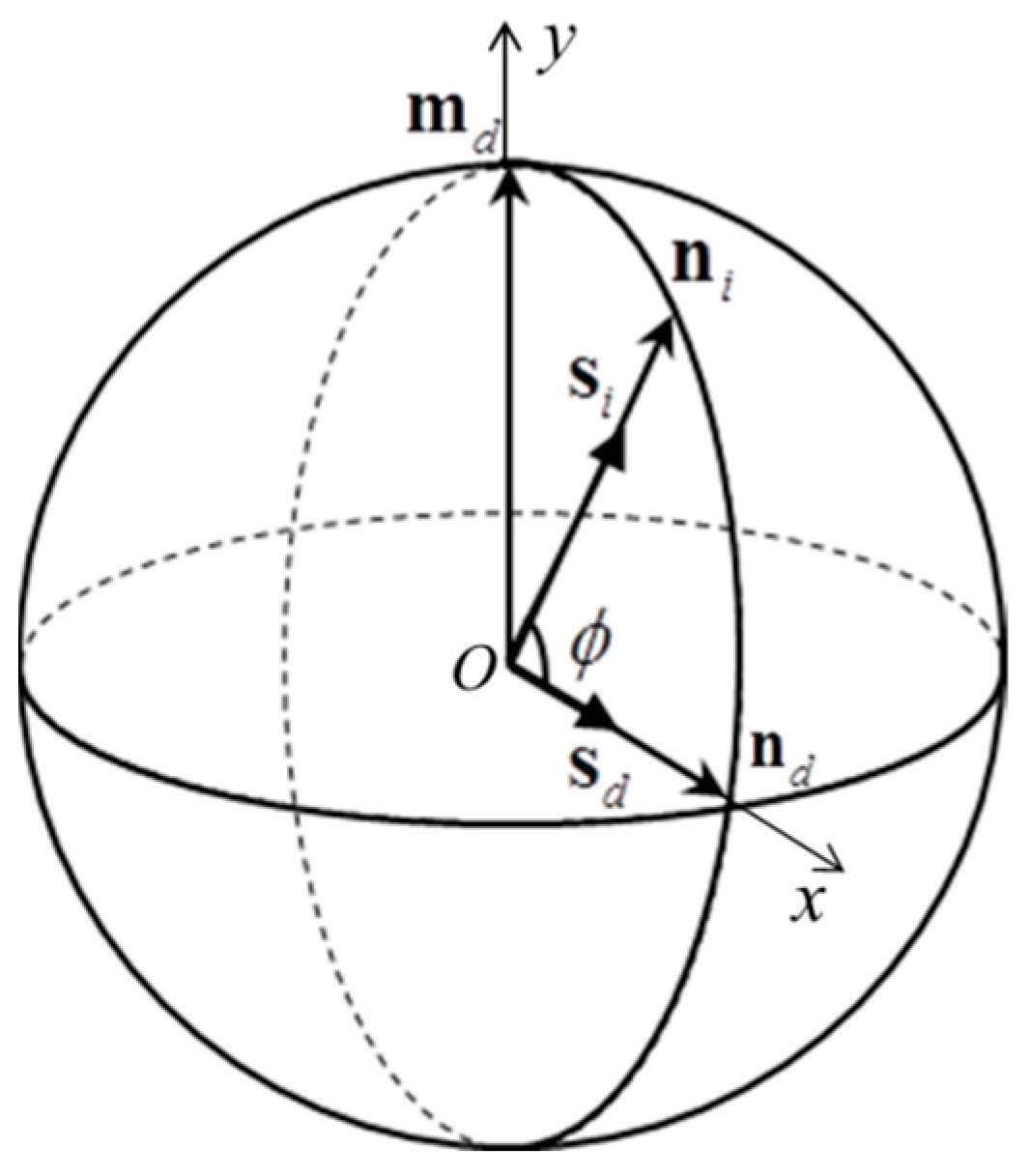
For bringing to light some relevant aspects of the rule of composition (24) of the Poincaré vectors of the input SOP and of the diattenuator, it is useful to decompose the output SOP along the Poincaré axis of the diattenuator, ${\mathbf{n}}_d$, and perpendicular to it, ${\mathbf{m}}_d$ (Figure 1), seeking the longitudinal and transversal effects of the diattenuator. Projecting Equation (27) on the axis of the diattenuator, one obtains the following [22]:

$$\begin{gathered} p_o{\mathbf{n}}_o.{\mathbf{n}}_d=\left[\frac{p_d{\mathbf{n}}_d+p_i{\mathbf{n}}_i}{1+p_d{\mathbf{n}}_d.p_i{\mathbf{n}}_i}+\frac{{\gamma }_d}{{\gamma }_d+1}\frac{p_d{\mathbf{n}}_d(p_d{\mathbf{n}}_d.p_i{\mathbf{n}}_i)-p_i{\mathbf{n}}_i{p}_d^2}{1+p_d{\mathbf{n}}_d.p_i{\mathbf{n}}_i}\right]{\mathbf{n}}_d \\ =\frac{p_d+{\mathbf{n}}_d.p_i{\mathbf{n}}_i}{1+p_d{\mathbf{n}}_d.p_i{\mathbf{n}}_i}=\frac{p_d+p_i\cos \varphi }{1+p_d{p}_{i}co\mathbf{s}\varphi } \end{gathered}$$

(30)

where $\varphi$ is the azimuth of the Poincaré vector of the input SOP with respect to the Poincaré vector of the diattenuator (Figure 1). The second term in the right-hand side of the gyrovector composition law is annihilated in this projection. The longitudinal effect of the diattenuator corresponds solely to the first term of the composition law, which here takes the form of the composition law of parallel gyrovectors.

The projection perpendicular to the Poincaré axis, ${\mathbf{n}}_d$, of the device (i.e., on ${\mathbf{m}}_d$) is as follows:

$$\begin{gathered} p_o{\mathbf{n}}_o.{\mathbf{m}}_d=\left[\frac{p_d{\mathbf{n}}_d+p_i{\mathbf{n}}_i}{1+p_d{\mathbf{n}}_d.p_i{\mathbf{n}}_i}+\frac{{\gamma }_d}{{\gamma }_d+1}\frac{p_d{\mathbf{n}}_d(p_d{\mathbf{n}}_d.p_i{\mathbf{n}}_i)-p_i{\mathbf{n}}_i{p}_d^2}{1+p_d{\mathbf{n}}_d.p_i{\mathbf{n}}_i}\right]{\mathbf{m}}_d \\ =\frac{{\gamma }_d{p}_i{\mathbf{n}}_i+p_i{\mathbf{n}}_i-{\gamma }_d{p}_d^2{p}_i{\mathbf{n}}_i}{({\gamma }_d+1)(1+p_d{\mathbf{n}}_d.p_i{\mathbf{n}}_i)}{\mathbf{m}}_d=\frac{\left(1+1/{\gamma }_d\right)p_i{\mathbf{n}}_i.{\mathbf{m}}_d}{({\gamma }_d+1)(1+p_d{\mathbf{n}}_d.p_i{\mathbf{n}}_i)} \\ =\frac{p_i |{\mathbf{n}}_i\times {\mathbf{n}}_d|}{{\gamma }_d(1+p_d{\mathbf{n}}_d.p_i{\mathbf{n}}_i)}=\frac{p_i\sin \varphi }{{\gamma }_d(1+p_d{p}_i\cos \varphi )}=\frac{p_i\sqrt{1-p_d^2}\sin \varphi }{1+p_d{p}_i\cos \varphi } \end{gathered}$$

(31)

From these projections, we obtain the azimuth $\psi$ of the output SOP with respect to the axis of the diattenuator:

$$tg\psi =\frac{p_i\left|{\mathbf{n}}_i\times {\mathbf{n}}_d\right|}{{\gamma }_d(p_i{\mathbf{n}}_i.{\mathbf{n}}_d+p_d)}=\frac{p_i\sin \varphi \sqrt{1-p_d^2}}{p_i\cos \varphi +p_d}=\frac{\sin \varphi \sqrt{1-p_d^2}}{\cos \varphi +p_d/p_i}=\frac{\tan \varphi \sqrt{1-p_d^2}}{1+\frac{p_d}{p_i}\sec \varphi }$$

(32)

It is straightforward to show that $\tan \psi \le \tan \varphi$, i.e., that any state of polarization passing by the partial polarizer is pushed toward the Poincaré axis of the device.

This effect was first perceived by Pancharatnam [23], the young “virtuoso of the Poincaré sphere” (as Sir Michael Berry described him [24]): “The differential absorption of the two components will cause the state of the elliptic vibration to «move towards» the state of polarization of less absorbed component (a phrase which acquires a more vivid meaning in the Poincaré sphere representation)”. Lu and Chipman [14] established this effect in the frame of a Mueller matrix calculus, stressing the fact that “for completely polarized light the incident states are moved along the great circles toward the diattenuator axis, which is the state of the maximum transmittance.” Bearing in mind the technological progress in polarimetry [25], all these aspects can be readily verified in detail and in a large variety of situations. The corresponding effect in STR is known as “headlight effect” or “forward collimating effect” of a Lorentz boost, and it is described by the same equation, with $\varphi$ and $\psi$ as the azimuths of the particle seen by two observers moving uniformly with respect to each other, and with $\mathrm{v}$ and $\mathrm{u}$ instead of $p_i$ and $p_d$ [26].

5. The Global Effect of a Diattenuator

A further step naturally arising in developing the Poincaré paradigm (on this line) would be to establish which is the action of the Poincaré vector of a diattenuator on a whole manifold of incident SOPs, e.g., on all the states of partial polarization contained (represented) in an inner Poincaré spherical ball of radius $p_i$, ${\Sigma }_3^{p_i}$. From the previous calculi, we have already seen that all these states will be pushed by the diattenuator forward and toward its Poincaré axis. But this action is drastically limited by the nonoverpolarization constraint, lightly speaking by the walls of the sphere. Bearing in mind that the Poincaré axis of the device constitutes a symmetry axis of its action, it is expected that the corresponding emerging SOPs should be contained in an ovoid ball (possibly a solid ellipsoid), which is oblate because of two adverse actions, i.e., the “pressing of the diattenuator” and the “resistance of the walls of the sphere”. Indeed, this is the case, and we have established the analytical equation of this ellipsoid at the beginning in terms of the hyperbolic parameter $\eta$ of the diattenuator [27]. Stepwise, we have passed to the Poincaré vectors of SOPs and devices, fitting the analytic description and equations to the proper terms of the geometrical description in the Poincaré ball [22,28].

Here, we have to emphasize that another line, very important for the polarimetry and polarimetric technologies, was developed using the Poincaré sphere representation in a very different sense, namely, in analyzing, in the Mueller matrix formalism, how various Mueller matrices deform the surface of completely polarized light, i.e., the surface ${\Sigma }_2^1$ of the Poincaré sphere. By the action of a Mueller matrix, the surface ${\Sigma }_2^1$ of the sphere of radius one (completely polarized light) transforms in a, generally more or less irregular, closed surface, which was called DoP (degree of polarization surface) [29] or P surface [30,31]. “For a given Mueller matrix, the degree of polarization surface is defined by moving each point on the unit Poincaré sphere radially inward, until its distance from the origin equals the output state degree of polarization for the corresponding input state. DoP maps and surfaces represent the variation of depolarization of a Mueller matrix for all fully polarized incident states” [29]. An exhaustively up-to-date presentation of this problem is given in [2].

In some of our papers, we have also used the DoP term for our ellipsoid, which is a source of confusion. With the term DoP being already adjudicated, we have to search another distinctive term, e.g., ellipsoidal Poincaré ball (EPB).

With Equations (31) and (32), the expression of the Poincaré vector of the emergent light from the diattenuator may be put in the following forms:

$$p_o{\mathbf{n}}_o=\frac{p_d+p_i{\mathbf{n}}_i.{\mathbf{n}}_d}{1+p_d{\mathbf{n}}_d.p_i{\mathbf{n}}_i}{\mathbf{n}}_d+\frac{p_i|{\mathbf{n}}_i\times {\mathbf{n}}_d|}{{\gamma }_d(1+p_d{\mathbf{n}}_d.p_i{\mathbf{n}}_i)}{\mathbf{m}}_d$$

(33)

$$p_o{\mathbf{n}}_o=\frac{p_d+p_i\cos \varphi }{1+p_d{p}_i\cos \varphi }{\mathbf{n}}_d+\frac{p_i\sqrt{1-p_d^2}\sin \varphi }{1+p_d{p}_i\cos \varphi }{\mathbf{m}}_d$$

(34)

In the first term on the right hand side of these equations, one sees that the projection of the incident Poincaré vector along the axis of the diattenuator simply adds up (up to the denominator) with the Poincaré vector of the diattenuator; the perpendicular projection is affected by the Lorentz factor of the device—one of the multitude of “quasi-relativistic” effects that originate in the analogy of Equations (21) and (23).

We now establish which is the geometric locus of the tops of all the Poincaré vectors of the exit SOPs, ${\mathbf{s}}_o=p_o{\mathbf{n}}_o$, for a given diattenuator, ${\mathbf{s}}_d=p_d{\mathbf{n}}_d$, and a given modulus, $p_i$, of the input SOPs, ${\mathbf{s}}_i=p_i{\mathbf{n}}_i$, i.e., how a given diattenuator transforms an inner Poincaré ball of incident SOPs, ${\Sigma }_3^{p_i}$.

In a system of Cartesian coordinates associated with the sphere, as in Figure 1, the coordinates of this geometric locus in the plane determined by the Poincaré vectors of the incident SOP and of the diattenuator are as follows:

$$x=\frac{p_d+p_i\cos \varphi }{1+p_d{p}_i\cos \varphi }\hspace{0.17em}y=\frac{p_i\sqrt{1-p_d^2}\sin \varphi }{1+p_d{p}_i\cos \varphi }$$

(35)

By eliminating the parameter $\varphi$, one obtains the equation of a conic:

$$x^2\left(1-p_d^2{p}_i^2\right)+y^2\left(1-p_d^2\right)-2x{p}_d\left(1-p_i^2\right)+p_d^2-p_i^2=0,$$

(36)

more precisely, an ellipse with the center displaced from origin of the Poincaré ball along the Poincaré axis of the dichroic device ${\mathbf{n}}_d$:

$${\left[x-\frac{p_d\left(1-p_i^2\right)}{1-p_d^2{p}_i^2}\right]}^2+\frac{y^2\left(1-p_d^2\right)}{1-p_d^2{p}_i^2}=\frac{p_i^2{\left(1-p_d^2\right)}^2}{{\left(1-p_d^2{p}_i^2\right)}^2}$$

(37)

If we want to see how a whole inner spherical Poincaré ball, ${\Sigma }_3^{p_i}$, of SOPs is modified by the action of the dichroic device of Poincaré vector, ${\mathbf{s}}_d=p_d{\mathbf{n}}_d$, we have to rotate the circular section $({\mathbf{n}}_d$, ${\mathbf{m}}_d)$ around the ${\mathbf{n}}_d$ axis, in Figure 1. The conclusion is that the diattenuator transforms the spherical ball of SOPs, ${\Sigma }_3^{p_i}$, in the ellipsoidal ball (solid ellipsoid):

$${\left[x-\frac{p_d(1-p_i^2)}{1-p_d^2{p}_i^2}\right]}^2+\frac{y^2(1-p_d^2)}{1-p_d^2{p}_i^2}+\frac{z^2(1-p_d^2)}{1-p_d^2{p}_i^2}=\frac{p_i^2{(1-p_d^2)}^2}{{(1-p_d^2{p}_i^2)}^2}$$

(38)

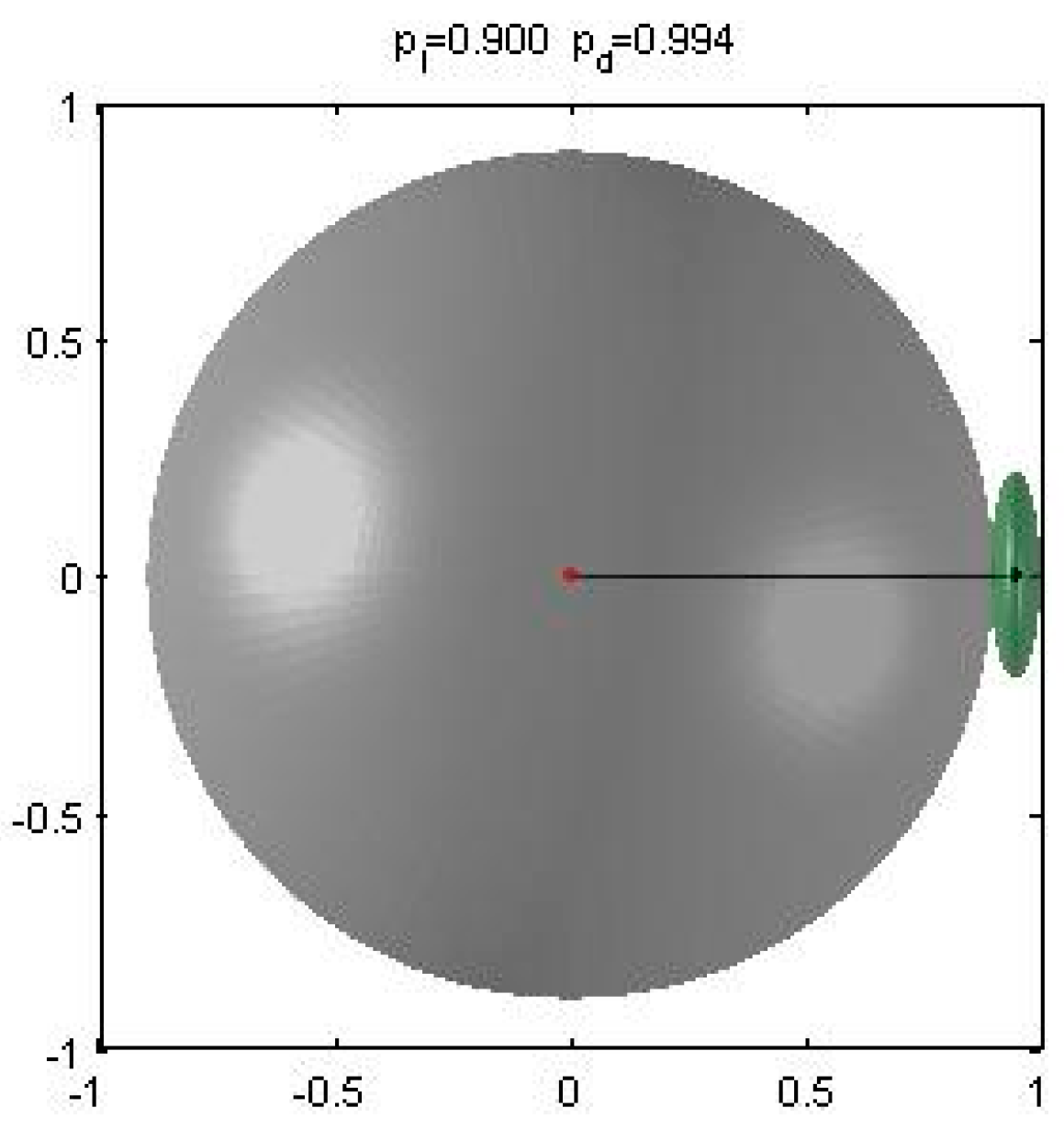
This is an oblate ellipsoid of rotation. The detailed calculus and the properties of this ellipsoid are given by various approaches, e.g., in [27,28]. In [28], we have illustrated in detail the behavior of the ellipsoidal Poincaré ball (EPB) at the border of the space in which it is imprisoned because of the condition of non-overpolarizability, i.e., at the walls, ${\Sigma }_2^1$, of the unit Poincaré ball. We review one of these limit situations. In Figure 2, we have considered a very strong diattenuator ($p_d=0.994$) acting on a large ($p_i=0.900$) inner ball ${\Sigma }_3^{p_i}$ of incident SOPs. All the incident SOPs are pushed forward and towards the Poincaré axis of the device. Moreover, they are all pushed outward from the sphere because the diattenuator is very strong ($p_d=0.994$), it is practically a pure polarizer. It totally polarizes any incident SOP, and it transforms any incident SOP into its major eigenstate. Very little dispersion of the output SOPs around the top of its Poincaré vector, ${\mathbf{s}}_d=p_d{\mathbf{n}}_d$, is allowed by such a strong device. All these things are natural in polarization theory. All these things seem “bizarre and counterintuitive” in their counterparts in STR. Certainly, they are not more counterintuitive than the second postulate. We could digress here toward the connections with the hyperbolic geometry, Poincaré disk, or even to the world, first imagined by Poincaré, of some virtual beings, whose universe is reduced to a sphere with finite radius, today called as “Poincarites”. But the aim of this paper is to avoid any collateral mathematics, and to show, as softly and intuitively as possible, how naturally the restriction (19) works in the polarization theory.

6. The Enpolarization/Depolarization Illustrated on the Poincaré Sphere

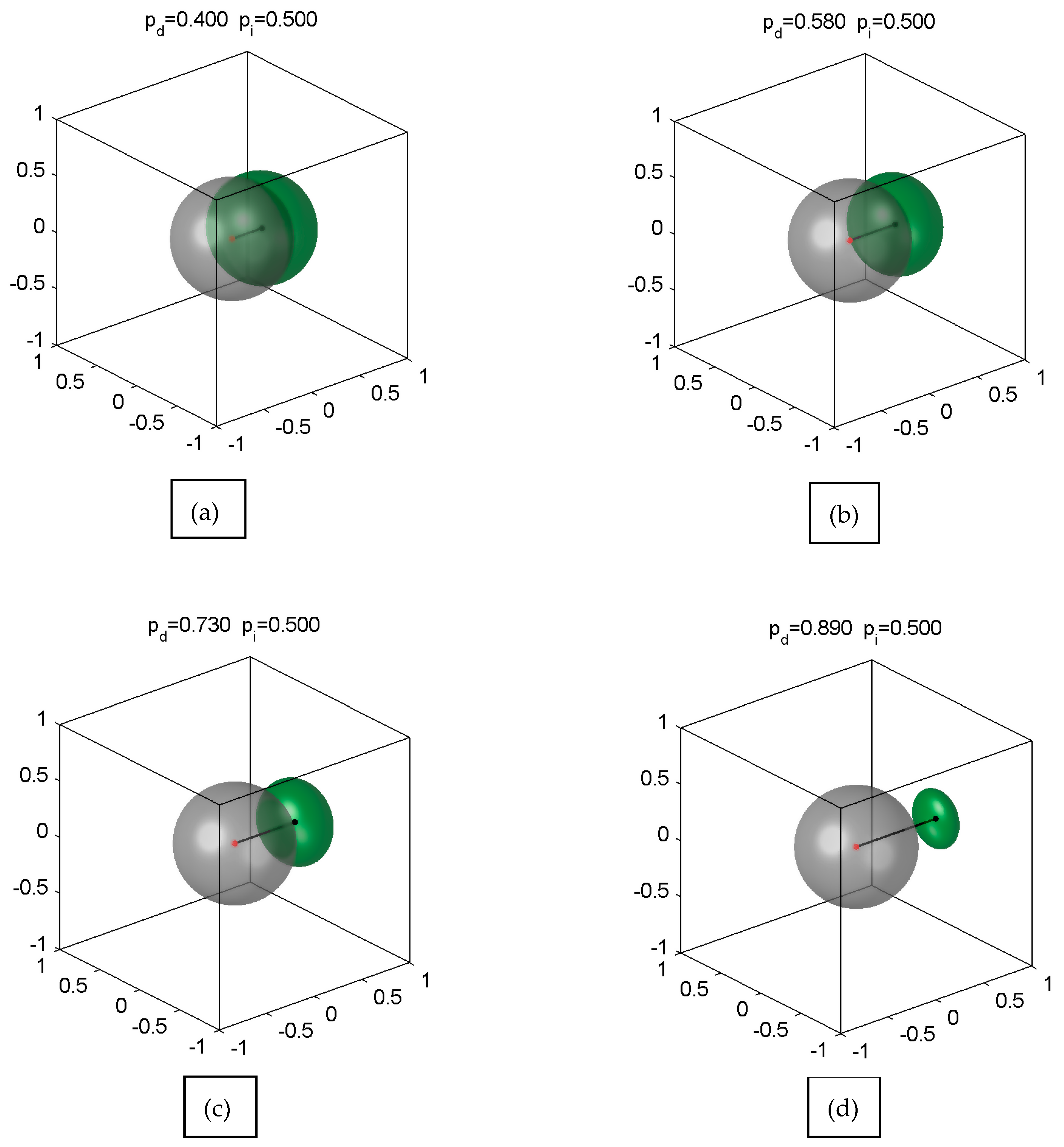
In this section, we shall illustrate how looks in the Poincaré ball the classical problem of depolarization/enpolarization given by deterministic devices [32], ref. [2], referring all along to diattenuators. In Figure 3, we have chosen some adequate values of the Poincaré parameters, for the clearest illustration of this effect: a moderate value of the radius of inner Poincaré ball of the input SOPs $(p_i=0.5)$. We shall increase, step by step, the strength of the dichroic device (its degree of dichroism), in a moderate range $(p_d\in 0.4–0.9)$. The diattenuator pushes all the incident SOPs of the ball ${\Sigma }_3^{p_i}$ along its axis (major eigenstate) i.e., in Figure 3, the line traced by the centers of ${\Sigma }_3^{p_i}$ (gray) and of the resulting EPB (green). But its effect on various SOPs is very different.

In Figure 3, the frontal part of the EPB overpasses the borders of the ball ${\Sigma }_3^{p_i}$ of the incident SOPs. Evidently, all these states are enpolarized (the output SOPs have a degree of polarization greater than the corresponding input SOPs). But not only these states are enpolarized. The SOPs situated in the frontal hemisphere of the ${\Sigma }_3^{p_i}$ ball are pushed in regions of the Poincaré ball ${\Sigma }_3^1$ corresponding to a greater degree of polarization. Their Poincaré vectors are, broadly speaking, oriented in the sense of the Poincaré axis of the diattenuator. The device acts “additively”, (“constructively”) on them. They are enpolarized as strong as their axes near to the parallelism with the diattenuator axis (smaller the angle $\varphi$). The most enpolarized incident SOP is that whose Poincaré axis is parallel with that of the device $({\mathbf{s}}_i\uparrow \uparrow {\mathbf{s}}_d)$. It reaches a maximum of the polarization degree after passing the diattenuator.

On the contrary, the SOPs situated in the rear hemisphere of the ${\Sigma }_3^{p_i}$ ball are pushed in regions near the center of the Poincaré ball ${\Sigma }_3^1$, i.e., corresponding to a smaller degree of polarization. All these SOPs are more or less antagonist with the device and are more or less depolarized by the device (Figure 3a).

A critical situation is presented in Figure 3b. By increasing the strength of the diattenuator $(p_d=0.58)$, it succeeds in pushing all the antagonist input SOPs beyond the center of the Poincaré ball ${\Sigma }_3^1$. The most antagonist input SOP $({\mathbf{s}}_i\uparrow \downarrow {\mathbf{s}}_d)$ touches the center of the Poincaré ball. It is completely depolarized. The whole EPB is situated in the right side (Figure 3b) of the center of the Poincaré ball ${\Sigma }_3^1$. For the antagonistic input SOPs, it is a turning point. After passing through the device, all of them are now partially polarized on the side of Poincaré axis of the diattenuator. By increasing the degree of dichroism of the device $(p_d=0.73)$, more SOPs of the input inner sphere ${\Sigma }_3^{p_i}$ are enpolarized, in the sense of the diattenuator axis (Figure 3c).

Another representative situation is presented in Figure 3d. The dichroic device is strong enough $(p_d=0.89)$ for pushing all the incident SOPs out of their sphere ${\Sigma }_3^{p_i}$. It converts the most antagonistic input SOP $({\mathbf{s}}_i\uparrow \downarrow {\mathbf{s}}_d)$ to its polarization structure $({\mathbf{s}}_o\uparrow \uparrow {\mathbf{s}}_d)$.

The expression of the degree of polarization of the output SOP, $p_o$, can be obtained either from Equation (17) or from Equation (34). The computational advantage of Equation (34) is striking. It is straightforward to calculate $p_o$ as the square root of the sum of the square of the components of $p_o{\mathbf{n}}_o$ along the two orthogonal unit vectors ${\mathbf{n}}_d$ and ${\mathbf{m}}_d$:

$$\begin{gathered} p_o^2=\frac{{\left(p_d+p_i\cos \varphi \right)}^2+{\left(p_i\sqrt{1-p_d^2}\sin \varphi \right)}^2}{{\left(1+p_d{p}_i\cos \varphi \right)}^2} \\ =\frac{p_i^2+p_d^2+2p_i{p}_d\cos \varphi -p_i^2{p}_d^2{\sin }^2\varphi }{{\left(1+p_d{p}_i\cos \varphi \right)}^2} \\ =\frac{{\left(1+p_d{p}_i\cos \varphi \right)}^2-1+p_i^2+p_d^2-p_i^2{p}_d^2}{{\left(1+p_d{p}_i\cos \varphi \right)}^2}=1-\frac{(1-{p_d}^2)(1-{p_i}^2)\hspace{0.17em}}{{\left(1+p_i{p}_d\cos \varphi \right)}^2} \end{gathered}$$

(39)

$$p_o={\left[1-\frac{(1-{p_d}^2)(1-{p_i}^2)\hspace{0.17em}}{{\left[1+p_i{p}_d\cos \varphi \right]}^2}\right]}^{1/2}$$

(40)

where $\varphi$ is the angle between the Poincaré vectors of the input SOP and of the diattenuator. This formula was first established in the frame of a pure algebraic Mueller matrix approach in [33]. Our deduction is a Poincaré geometrical one, based, in last instance, on the condition of non-overpolarizability (19), i.e., the imprisonment of Poincaré vectors of the SOPs and diattenuators in the ${\Sigma }_3^1$ Poincaré ball. From (40) it is immediately that $p_o\le 1$.

This is a formula referring to each individual state. The degree of polarization $p_o$ of the output SOP depends on the degree of polarization $p_i$ of the input SOP, on the degree of dichroism $p_d$ of the device and on the degree of resemblance ($\cos \varphi ={\mathbf{n}}_i.{\mathbf{n}}_d\in \left[1,0\right]$), or adversity ($\cos \varphi ={\mathbf{n}}_i.{\mathbf{n}}_d\in \left[0,-1\right]$) between them.

When $\varphi =0$, that is, the diattenuator axis is parallel with that of the input SOP $({\mathbf{s}}_d\uparrow \uparrow {\mathbf{s}}_i)$, the degree of polarization of the output SOP reaches its maximum value:

$$p_o=\frac{p_i+p_d\hspace{0.17em}}{1+p_i{p}_d}$$

(41)

Not accidentally, this is the rule of addition of the parallel velocities in STR.

When $\varphi =\pi$, the diattenuator axis is antiparallel with that of the input SOP $({\mathbf{s}}_d\uparrow \downarrow {\mathbf{s}}_i)$ and the degree of polarization of the output SOP reaches its minimum:

$$p_o=\frac{\left|p_i-p_d\right|\hspace{0.17em}}{1-p_i{p}_d}$$

(42)

Here, there are two situations. Both of them correspond to input SOPs situated along the axis of the diattenuator, in opposition with this one. The output SOP $({\mathbf{s}}_o\uparrow \uparrow {\mathbf{s}}_i)$ in Figure 3b or $({\mathbf{s}}_o\uparrow \uparrow {\mathbf{s}}_d)$ in Figure 3c is decided by the competition between the strengths of the input SOP and of the diattenuator (i.e., the degree of polarization and the degree of dichroism, respectively).

By the end of these theoretical aspects of the problems of the Poincaré sphere, Pauli algebraic approaches and Lorentz boosts in polarization optics, we want to emphasize that in recent times some spectacular applications, even of micro- and nano-optical engineering, have been reported in these fields [34,35,36,37,38]. These papers throw fresh light and open new perspectives on the classical problems that we have presented above.

7. Conclusions

In polarization optics, there are two principal lines on which the Poincaré geometric representation was intensively developed.

One of them refers to the, very general, analysis of the action of various devices/media (mainly indeterministic) on polarized light. This is strongly connected with the algebraic formalism of Mueller matrices. In this field, a device/media is defined as depolarizing if it transforms the Poincaré sphere ${\Sigma }_3^1$ (i.e., the manifold of totally polarized states), in an inner surface of the sphere, the so-called P or DoP surface. The field is exhaustively and in an up-to-date manner dealt with in [2].

The other one, which we have presented above, is more restrictive from a polarimetric viewpoint. It refers to the interaction between deterministic devices/media and polarized light. In this field, a device/medium is called depolarizing, if it reduces the degree of polarization of the input light, and enpolarizing, if it increases the degree of polarization of the input light.

The action of the birefringent devices/media (represented by unitary operators) on polarized light has a simple effect in the geometric representation: a rotation around the Pauli/Poincaré axis of the device, on the Poincaré sphere, or in the Poincaré ball.

The action of a diattenuator (represented by a Hermitian operator)—that we have analyzed and illustrated above in detail—is much more complex. The condition of non-overpolarizability acts here drastically. Both the Poincaré vectors of the diattenuator and of input light are “prisoners” of the Poincaré ball ${\Sigma }_3^1$, and they are forced to combine in such a way that their resultant, the Poincaré vector of the emergent light, should remain in the Poincaré ball. Not surprisingly, their law of addition is the same as that of admissible relativistic velocities, which are themselves imprisoned in a sphere of radius one (in adequate units of speed of light), i.e., a Poincaré sphere. But, while the restriction of non-overpolarizability and all its consequences illustrated above are quite natural, the restriction of the second STR postulate and its consequences (especially the paradoxes) remain counterintuitive. The main (underground) aim of this review paper is to make the counter intuitive aspects of STR more familiar, via their counterparts in the polarization theory. We have to note that there are many two-state systems (as the deterministic polarization devices), which are naturally subjected to the same restriction.

The most suitable algebraic approach to this line of Poincaré sphere development is that of Pauli algebra because the Pauli axes of the SOPs and device operators coincide with their Poincaré geometric axes. This approach leads straightly to the Pauli–Poincaré vector of output light and of the gain of the device.

The geometric locus of the output SOP vectors for all the input SOPs contained in an inner Poincaré sphere is a solid oblate ellipsoid that we have denominated—for the mentioned distinct reasons—EPB (ellipsoidal Poincaré ball). The deformation of various input SOPs spheres in the corresponding EPBs provides a deeper insight into the action of deterministic devices on the polarized light as well as in their STR equivalents.